Robust Constrained Multi-Objective Guidance of Supersonic Transport Landing Using Evolutionary Algorithm and Polynomial Chaos

Abstract

Landing of supersonic transport (SST) suffers from a large uncertainty due to its highly sensitive aerodynamic properties in the subsonic domain, as well as the wind gusts around runways. At the vehicle design stage, a landing trajectory optimization under wind uncertainty in a multi-objective solution space is desired to explore the possible trade-off in its key flight performance metrics. The proposed algorithm solves this robust constrained multi-objective optimal control problem by integrating non-intrusive polynomial chaos expansion into a constrained evolutionary algorithm. The computationally tractable optimization is made possible through the conversion of a probabilistic problem into an equivalent deterministic representation while maintaining a form of the multi-objective problem. The generated guidance trajectories achieve a significant reduction of the uncertainty in their terminal states with a marginal modification in the control history of the deterministic solutions, validating the importance of the consideration of robustness in trajectory optimization.

1. Introduction

Supersonic transport (SST), or supersonic airliners, have been gaining interest as the next paradigm shift in transport. Based on the optimal aerodynamic properties in the supersonic domain, SST typically adopts delta wings with a large sweep-back angle. However, such wing shapes lead to an inevitable trade-off of poor aerodynamic properties in the low-speed domain [1,2]. This is mitigated by a high angle of attack at takeoff and landing. Thus, the control system is vulnerable to meteorological uncertainty, such as wind gusts (microbursts) on a runway [3], owing to the high sensitivity of its aerodynamic properties. This motivates designers to develop a robust SST landing-trajectory design under uncertainty, even for open-loop control at the preliminary design phase. Additionally, multiple objective functions, such as fuel efficiency and environmental impact, must be taken into account to make a decision on the vehicle configuration.

Numerous works on the trajectory optimization of aerospace vehicles have dealt with the uncertainty [4,5,6,7,8,9,10,11,12,13,14,15,16,17,18]. A simple non-intrusive approach is based on the Monte Carlo (MC) method, although this approach typically suffers from the curse of dimensionality. In order to make the computation time tractable, additional modifications are often required [4,5]. Linear covariance analysis [6], which is developed from filtering theory, has been widely used to capture the propagation of uncertainty in the linear dynamical system. Several studies have proposed robust trajectory-optimization methods using this technique [8,9]. Finally, generalized polynomial chaos expansion (PCE) [10,11], which was originally developed as a mathematical tool for uncertainty quantification, has been demonstrated to be a suitable method for nonlinear dynamics [12,13,14,15,16,17,18]. The majority of these works are, however, focusing on single-objective problems. Such problem formulations end up solving a large-scale nonlinear programming (NLP), and the direct application of the single-objective NLP-based methods to obtain the multi-objective Pareto-front is challenging due to the significant increase in the computational complexity.

Optimization over a multi-objective space is important for aerospace systems, particularly at the early stage of conceptual design. As the system-level performances of the aerospace vehicles are typically coupled with the trajectory design, multi-objective optimal control [19] has been a widely investigated topic. In the context of the landing/takeoff-trajectory designs of civilian aircraft, several metaheuristics-based methods have been developed to seek the trade-off of environmental effects (noise abatement), economic efficiencies, and other flight properties [20,21,22]. Kanazaki et al. developed an integrated flight control optimization method with an efficient aerodynamic flight dynamics simulation for the SST’s optimal control, using a multi-objective evolutionary algorithm (MOEA). The Kriging model-assisted aerodynamic estimation was implemented in the flight simulation to optimize the landing trajectory of an aircraft whose high-fidelity aerodynamic properties are critically coupled to its trajectory and control analysis [23,24]. The limitation of these studies is in the deterministic problem transcription, as nominal control sequences may follow an overly aggressive flight-control design under large uncertainties.

Multiple studies have addressed robust multi-objective trajectory optimization problems. One approach is to transcribe the probabilistic problem into a minimization of the lower expectations using surrogate modeling [25]. Furthermore, Refs. [26,27,28,29] defined the problem-specific robustness indices (e.g., the difference between objectives in the worst and best scenarios), which are regarded as an objective among the other performance metrics. However, such methods cannot capture the exact landscape of the probability distribution of the uncertain parameters. This would return overly conservative solutions, and the worst scenarios are sometimes not well-defined for unbounded probability distributions. Gonzalez et al. solved a multi-objective optimization of an aircraft path planning under the meteorological uncertainty based on MOEA and ensemble prediction systems [29], while the constraint-handling scheme was not generalized.

The aim of this study is to bridge these two philosophies in trajectory design: robust guidance under generalized constraints and multi-objective optimization. Our objective is to incorporate robustness against uncertainty into the constraints, rather than integrating it into the objectives. This approach is intended to enhance the versatility of the problem formulation, making it more suitable for a broad spectrum of optimal control problems that contain a number of constraints. The robust constrained multi-objective optimal control problems are not only critical to the conceptual study of the SST design but also applicable to the designs of many other new aerospace systems operated under uncertain environments, such as Mars airplanes [30], balloon probes for planetary exploration [31], or space debris reentering the atmosphere [32].

This paper has three key contributions. First, the robust optimal control formulation developed by Li et al. [12] is expanded to the multi-objective problem. The non-intrusive PCE is embedded into the constrained MOEA to solve this problem, which enables the efficient handling of stochastic constraints. Instead of using NLP-based methods that process constraints simultaneously, the constraints are processed sequentially, and the violations are evaluated by the Pareto ranking-based evolutionary algorithm. Additionally, extending the previous work by the authors [33], the benefit of the proposed method in the SST landing when encountering unexpected gusts of wind is demonstrated. The MC simulation validates the advantageous flight profile of the obtained robust control history against wind uncertainty, compared to the nominal solution. It is shown that a subtle change in the control history can significantly improve the robustness of the generated trajectories. Finally, the proposed approach enables the depiction of the uncertainty-aware non-inferior solution surface. The translational shift of the solution surface, coupled with variations in constraint satisfaction robustness, introduces a new perspective of examining the trade-offs in mission objectives and their resilience.

The subsequent sections of this paper are structured as follows. In Section 2, robust constrained multi-objective optimal control and its reformulation to the deterministic problem via the PCE are discussed. In Section 3, a case study of the optimal guidance for the SST landing is elaborated, followed by its constraint allocation. In Section 4, the obtained robust solutions are presented and compared with the nominal solutions, which is followed by the validation of the robust control profile through MC simulation. Lastly, Section 5 concludes the work.

2. Robust Constrained Multi-Objective Trajectory Optimization

The aim of this paper is to consider the multi-objective solution space of the optimal trajectories, where the time-invariant open-loop control is resilient to uncertain parameters. The generality of the problem is maintained throughout this section so that the application to the other vehicle configurations can be easily performed.

2.1. Problem Formulation

First, the following multi-objective optimal control problem is introduced under a deterministic environment with continuous-time dynamics:

$$\begin{array}{cc}\hfill \underset{\mathbf{x}\left(t\right),\mathbf{u}\left(t\right)}{min}& \{{\mathcal{J}}_1,\dots ,{\mathcal{J}}_N\}\hfill \end{array}$$

(1a)

$$\begin{array}{cc}\hfill \mathrm{subject}\mathrm{to}& \dot{\mathbf{x}}\left(t\right)=\mathit{F}(\mathbf{x}\left(t\right),\mathbf{u}\left(t\right),t)\hfill \end{array}$$

(1b)

$$\begin{array}{cc}\hfill & \mathit{g}\left(\mathbf{x}\right(t),\mathbf{u}(t),t)\le \mathbf{0}\hfill \end{array}$$

(1c)

$$\begin{array}{cc}\hfill & \mathit{h}\left(\mathbf{x}\right(t),\mathbf{u}(t),t)=\mathbf{0},\hfill \end{array}$$

(1d)

where the dynamics of the system are defined in Equation (1b), and Equations (1c) and (1d) are the set of inequality and equality constraints, respectively. Furthermore, each objective function is expressed as follows [34]:

$$\begin{array}{c}\hfill \begin{array}{c}\hfill {\mathcal{J}}_n=\Phi (\mathbf{x}\left(t_f\right),t_f)+{\int }_{t_0}^{t_f}L(\mathbf{x}\left(t\right),\mathbf{u}\left(t\right),t)dt\forall n=1,\dots ,N,\end{array}\end{array}$$

(2)

where the first term is the terminal cost (Mayer’s term), and the second is the running cost along the path (Lagrange’s term).

Considering the uncertainty (probabilistic parameters) in Equation (1), the problem can be rewritten as follows:

$$\begin{array}{cc}\hfill \underset{\mathbf{x}(t,\mathit{\xi }),\mathbf{u}\left(t\right)}{min}& \{{\mathcal{J}}_1,\dots ,{\mathcal{J}}_n\}\hfill \end{array}$$

(3a)

$$\begin{array}{cc}\hfill \mathrm{subject}\mathrm{to}& \dot{\mathbf{x}}(t,\mathit{\xi })=\mathit{F}(\mathbf{x}(t,\mathit{\xi }),\mathbf{u}\left(t\right),t)\mathrm{a}.\mathrm{s}.\hfill \end{array}$$

(3b)

$$\begin{array}{cc}\hfill & \mathit{g}\left(\mathbf{x}\right(t,\mathit{\xi }),\mathbf{u}(t),t)\le \mathbf{0}\mathrm{a}.\mathrm{s}.\hfill \end{array}$$

(3c)

$$\begin{array}{cc}\hfill & \mathit{h}\left(\mathbf{x}\right(t,\mathit{\xi }),\mathbf{u}(t),t)=\mathbf{0}\mathrm{a}.\mathrm{s}.,\hfill \end{array}$$

(3d)

where $\mathit{\xi }$ is a vector of probabilistic parameters. The objectives are also rewritten as follows:

$${\mathcal{J}}_n=\Phi (\mathbf{x}(t_f,\mathit{\xi }),\mathbf{u}\left(t_f\right))+{\int }_0^{t_f}L(\mathbf{x}(t,\mathit{\xi }),\mathbf{u}\left(t\right),t)\mathrm{d}t\forall n=1,\dots ,N.$$

(4)

The constraints are satisfied a.s. (almost surely), rendering the probabilistic treatment of the constraints. Additionally, we can set $t=0$ without loss of generality. Note that $\mathit{\xi }$ is not an argument of $\mathbf{u}\left(t\right)$ as the open-loop robust optimizer is sought in this paper.

2.2. Reformulation to a Deterministic Problem

Problem Equation (3a) is equivalent to an infinite-dimensional deterministic problem owing to the existence of probabilistic parameters. However, this formulation can be converted into an equivalent finite-dimensional deterministic form [12]. First, we rewrite the stochastic static constraints as follows:

$$\begin{array}{cc}\hfill \underset{\mathbf{x}(t,\mathit{\xi }),\mathbf{u}\left(t\right)}{min}& \{{\mathcal{J}}_1,\dots ,{\mathcal{J}}_N\}\hfill \end{array}$$

(5a)

$$\begin{array}{cc}\hfill \mathrm{subject}\mathrm{to}& \dot{\mathbf{x}}(t,\mathit{\xi })=\mathit{F}(\mathbf{x}(t,\mathit{\xi }),\mathbf{u}\left(t\right),t)\mathrm{a}.\mathrm{s}.\hfill \end{array}$$

(5b)

$$\begin{array}{cc}\hfill & \mu \left(\mathit{g}\right(\mathbf{x}(t,\mathit{\xi }),\mathbf{u}\left(t\right),t\left)\right)\le \mathbf{0}\hfill \end{array}$$

(5c)

$$\begin{array}{cc}\hfill & \sigma \left(\mathit{g}(\mathbf{x}(t,\mathit{\xi }),\mathbf{u}\left(t\right),t)\right)\le {\mathit{\sigma }}_g\hfill \end{array}$$

(5d)

$$\begin{array}{cc}\hfill & \mu \left(\mathit{h}\right(\mathbf{x}(t,\mathit{\xi }),\mathbf{u}\left(t\right),t\left)\right)=\mathbf{0}\hfill \end{array}$$

(5e)

$$\begin{array}{cc}\hfill & \sigma \left(\mathit{h}(\mathbf{x}(t,\mathit{\xi }),\mathbf{u}\left(t\right),t)\right)\le {\mathit{\sigma }}_h.\hfill \end{array}$$

(5f)

In this formulation, the robustness of the constraint satisfaction under uncertainty is parameterized by the variance of the constraint functions. Replacing “a.s.” with the constraints on the mean and standard deviation allows us to statistically evaluate them, which is applicable to a wide range of robust optimal control problems because we can easily tune these parameters.

Next, we introduce the non-intrusive PCE [11] to transform a single probabilistic ordinary differential equation (ODE) into a bundle of deterministic ODEs. Given a nonlinear dynamical system in Equation (5b), solving this over a probabilistic distribution is difficult due to the high (or infinitely large) dimensionality. Instead, we approximate the state variable $\mathbf{x}(t,\mathit{\xi })$ to a linear combination of orthogonal basis functions $\varphi \left(\mathit{\xi }\right)$ with their respective coefficients $\tilde{\mathit{x}}\left(t\right)$. The two arguments of the state, t and $\mathit{\xi }$, are decoupled via this approximation as follows:

$$\begin{array}{c}\hfill \mathbf{x}(t,\mathit{\xi })\simeq \sum _{i=0}^p{\tilde{\mathit{x}}}_i\left(t\right){\varphi }_i\left(\mathit{\xi }\right),\end{array}$$

(6)

where i denotes the approximation order of the PCE, spanning from the zeroth order up to the p-th order. The orthogonal basis functions are characterized by the following property (orthogonality):

$$\begin{array}{c}\begin{array}{c}<{\varphi }_i\left(\mathit{\xi }\right),{\varphi }_j\left(\mathit{\xi }\right)>=\int {\varphi }_i\left(\mathit{\xi }\right){\varphi }_j\left(\mathit{\xi }\right)\rho \left(\mathit{\xi }\right)d\mathit{\xi }=<{\varphi }_i^2>{\delta }_{ij},\hfill \end{array}\end{array}$$

(7)

where $\rho \left(\mathit{\xi }\right)$ is the weight function (i.e., joint probability density function). For many popular probability distributions $\mathit{\xi }$, the corresponding orthogonal basis function $\varphi \left(\mathit{\xi }\right)$ has been determined [10].

Non-intrusive PCE provides the following formula for the coefficients ${\tilde{\mathit{x}}}_i\left(t\right)$:

$$\begin{array}{c}\hfill {\tilde{\mathit{x}}}_i\left(t\right)=\frac{1}{<{\varphi }_i^2\left(\mathit{\xi }\right)>}\int \mathit{x}(t,\mathit{\xi }){\varphi }_i\left(\mathit{\xi }\right)\rho \left(\mathit{\xi }\right)d\mathit{\xi }\end{array}$$

(8)

This equation is approximated using the full tensor-product numerical quadrature rule to compute ${\tilde{\mathit{x}}}_i\left(t\right)$ with a finite number of samples.

$$\begin{array}{c}\hfill {\tilde{\mathit{x}}}_i\left(t\right)=\sum _{s_1=1}^l\cdots \sum _{s_q=1}^l\mathbf{x}(t,{\xi }_{s_1},\dots ,{\xi }_{s_q})\frac{{\varphi }_i({\xi }_{s_1},\dots ,{\xi }_{s_q})}{<{\varphi }_i^2>}\prod _{j=1}^q{w}_j,\end{array}$$

(9)

where $\mathit{\xi }=[{\xi }_{s_1},\dots ,{\xi }_{s_q}]\in {\mathbb{R}}^q$; l is the number of quadrature points sampled in the range of $\mathit{\xi }$; and $w_j$ is the weight of each quadrature point. In summary, the above two formulas enable us to obtain ${\xi }_{s_1},\dots ,{\xi }_{s_q}$, ${\varphi }_i({\xi }_{s_1},\dots ,{\xi }_{s_q})$, and $w_j\forall j=1,\dots ,q$ automatically for many popular probability distributions $\mathit{\xi }$, given $p,q$, and l.

Additionally, $\mathbf{x}(t,{\xi }_{s_1},\dots ,{\xi }_{s_q})$ is a deterministic ODE with a constant parameter set because ${\xi }_{s_1},\dots ,{\xi }_{s_q}$ are the pre-defined values that correspond to the quadrature points. Therefore, given an initial condition, we can perform the numerical integration of the following trajectory:

$$\begin{array}{c}\hfill \begin{array}{cc}\hfill \dot{\mathbf{x}}(t,{\xi }_{s_1},\dots ,{\xi }_{s_q})& =\mathit{F}(\mathbf{x}(t,{\xi }_{s_1},\dots ,{\xi }_{s_q}),\mathbf{u}\left(t\right),t).\hfill \end{array}\end{array}$$

(10)

Based on this observation, the “a.s.” in Equation (5b) can be replaced with the following constraint.

$$\begin{array}{c}\hfill \dot{\mathbf{x}}(t,{\mathit{\xi }}_k)=\mathit{F}(\mathbf{x}(t,{\mathit{\xi }}_k),\mathbf{u}\left(t\right),t),k=1,\dots ,M.\end{array}$$

(11)

Given a control sequence $\mathbf{u}\left(t\right)$, the satisfaction of $M=l^q$ deterministic equations of motion (EoMs) in Equation (11) renders a statistical equivalence to the satisfaction of the stochastic EoM in Equation (5b) in a form that the optimization solver can handle. This conversion of a single EoM over a probability distribution to a finite number of deterministic EoMs is generalized as the trajectory ensemble [35].

In summary, the robust constrained multi-objective trajectory optimization problem in Equation (5) is rewritten in the following deterministic form.

$$\begin{array}{cc}\hfill \underset{\mathbf{x}(t,\mathit{\xi }),\mathbf{u}\left(t\right)}{min}& \{{\mathcal{J}}_1,\dots ,{\mathcal{J}}_N\}\hfill \end{array}$$

(12a)

$$\begin{array}{cc}\hfill \mathrm{subject}\mathrm{to}& \dot{\mathbf{x}}(t,{\mathit{\xi }}_k)=\mathit{F}(\mathbf{x}(t,{\mathit{\xi }}_k),\mathbf{u}\left(t\right),t),k=1,\dots ,M\hfill \end{array}$$

(12b)

$$\begin{array}{cc}\hfill & \mu \left(\mathit{g}\right(\mathbf{x}(t,\mathit{\xi }),\mathbf{u}\left(t\right),t\left)\right)\le \mathbf{0}\hfill \end{array}$$

(12c)

$$\begin{array}{cc}\hfill & \sigma \left(\mathit{g}(\mathbf{x}(t,\mathit{\xi }),\mathbf{u}\left(t\right),t)\right)\le {\mathit{\sigma }}_g\hfill \end{array}$$

(12d)

$$\begin{array}{cc}\hfill & \mu \left(\mathit{h}\right(\mathbf{x}(t,\mathit{\xi }),\mathbf{u}\left(t\right),t\left)\right)=\mathbf{0}\hfill \end{array}$$

(12e)

$$\begin{array}{cc}\hfill & \sigma \left(\mathit{h}(\mathbf{x}(t,\mathit{\xi }),\mathbf{u}\left(t\right),t)\right)\le {\mathit{\sigma }}_h.\hfill \end{array}$$

(12f)

Using the coefficients ${\tilde{\mathit{x}}}_i\left(t\right)$, the mean and standard deviation are computed as follows:

$$\begin{array}{cc}\hfill \mu \left(\mathbf{x}\right(t,\mathit{\xi }\left)\right)=& {\tilde{\mathbf{x}}}_0\left(t\right)\hfill \end{array}$$

(13)

$$\begin{array}{cc}\hfill \sigma \left(\mathbf{x}\right(t,\mathit{\xi }\left)\right)=& \sqrt{\sum _{i=1}^p<{\varphi }_i^2>{\tilde{\mathbf{x}}}_i^2\left(t\right)}\hfill \end{array}$$

(14)

We note that these formulas can also be used to evaluate other forms of probabilistic properties, such as chance constraints [36].

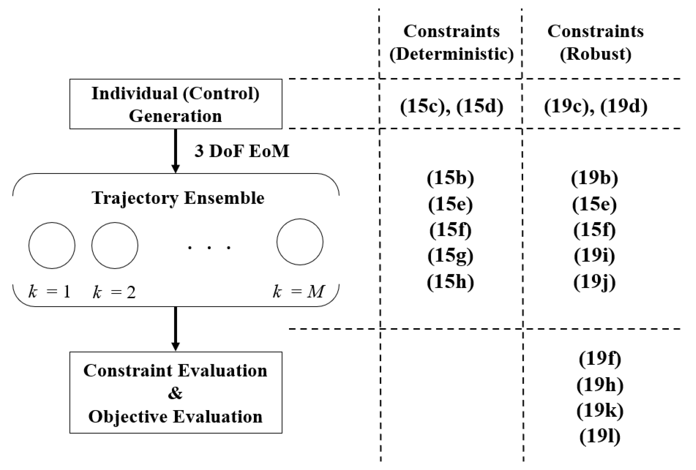
2.3. Global Optimization Method: Integration into the Constrained MOEA

The deterministic form of the robust constrained multi-objective optimal control problem in Equation (12) is solved via a constrained MOEA [37,38]. The constraint-handling scheme for this robust trajectory optimization problem is presented in Figure 1.

The constrained MOEA implemented in this study comprises three phases that process the constraints. First, when individuals are produced at each generation, we can set upper and lower bounds for the optimization (i.e., control) variables a priori. Second, given the control sequence, M ODEs are propagated to map the control sequence to the space of the objective functions and constraints, which automatically satisfy the dynamical constraints. Finally, the constrained MOEA evaluates the constraint violation, which is reflected in the population of the next generation. A holistic survey of the constraint-handling techniques in an EA is presented in Ref. [38]. Leveraging this three-staged constraint-handling scheme, we can solve for the robust formulation while maintaining its form of multi-objective optimization. The detail of the constraint handling for the SST landing trajectory optimization is described in Section 3.2.

3. SST Landing Trajectory Optimization

In this section, the optimal control problem for the SST landing is elaborated, which is then extended to the robust formulation. We consider the continuous descent operation (CDO), where we optimize the time history of $\delta e$. The dynamics, aerodynamic estimation, and constraints are developed based on the previous literature [24], while the proposed algorithm can be applied to any vehicle configuration. The inclusion of the thrust control is not in the scope of this paper because limiting the dimensionality of the control variables makes the difference in the nominal and robust control history more distinct. However, we note that the proposed algorithm can take any dimension of the control variable.

3.1. Deterministic Formulation

First, the baseline deterministic formulation is presented as follows:

$$\begin{array}{c}\mathrm{(15a)}& {\displaystyle \underset{\delta e\left(t\right)}{max}}\hspace{1em}\{t_f,x\left(t_f\right)\}\mathrm{subject}\mathrm{to}\\ \mathrm{(15b)}& \dot{\mathbf{x}}\left(t\right)=\left[\begin{array}{c}\dot{x}\\ \dot{z}\\ \dot{v_x}\\ \dot{v_z}\\ \dot{\theta }\\ \dot{\omega }\end{array}\right]=\left[\begin{array}{c}{v}_x\\ v_z\\ \frac{X}{m}-gsin\theta -\omega \frac{dz}{dt}\\ \frac{Z}{m}-gcos\theta -\omega \frac{dx}{dt}\\ \omega \\ \frac{T_{\theta }}{I_{yy}}\end{array}\right]\mathrm{(15c)}& -50.0{}^{\circ }\le \delta e\left(t\right)\le 10.0{}^{\circ },-35.9{}^{\circ }\le \delta e\left(0\right)\le -15.9{}^{\circ }\mathrm{(15d)}& \left|\delta e\right(t+1)-\delta e\left(t\right)|\le 2.0^{\circ }\mathrm{(15e)}& 0.1\le Ma\left(t\right)\le 0.5\mathrm{(15f)}& -5.0\le \alpha \left(t\right)\le 21.0^{\circ }\mathrm{(15g)}& \mathbf{x}\left(0\right)={\mathbf{x}}_0=\left[\begin{array}{c}{x}_0\\ z_0\\ v_{x0}\\ v_{z0}\\ {\theta }_0\\ {\omega }_0\end{array}\right]=\left[\begin{array}{c}0.0 \mathrm{m}\\ 1000.0 \mathrm{m}\\ 120.0 \mathrm{m}/\mathrm{s}\\ 0.0 \mathrm{m}/\mathrm{s}\\ 0.0{}^{\circ }\\ 0.0{}^{\circ }/\mathrm{s}\end{array}\right]\mathrm{(15h)}& z\left(t_f\right)=0.0 \mathrm{m}.\end{array}$$

In this paper, the maximization of the flight time $t_f$ and the flight range $x\left(t_f\right)$ are considered as two competing objectives. The dynamics of the SST in Equation (15b) are modeled in the x-z plane in the inertial frame with 3 degrees of freedom (DoF); $\theta$ and $\omega$ are the flight path angle and its angular velocity (measured counter-clockwise from the x-axis); $T_{\theta }$ is the pitch torque applied to the aircraft’s center of mass; and X and Z represent the total aerodynamics force acting on the SST in the x and z-direction, respectively.

The constraints of this problem are defined as follows. First, the range of the control inputs is defined in Equation (15c). Additionally, the maximum rate of change in the elevator angle is limited by Equation (15d) to avoid an unrealistic control profile. The elevator control is assumed to update the angle at a frequency of 2 Hz. Path constraints (15e) and (15f) limit the ranges of the feasible velocity and angle of attack. These ranges correspond to the approximation domain of the aerodynamic force. Finally, the initial and terminal conditions of the aircraft are defined in Equations (15g) and (15h), respectively. The trajectory propagation is terminated when the aircraft lands on the ground.

The configurations of the SST and physical parameters used for the simulations are summarized in

Table 1. Configurations of the SST and the physical parameters.

SST Configuration	Value
$m\left[\mathrm{kg}\right]$	15,000
$I_{yy}\left[{\mathrm{m}}^2·\mathrm{kg}\right]$	319,900
$S_{\mathrm{ref}}\left[{\mathrm{m}}^2\right]$	$43.446$
$l_{\mathrm{MAC}}\left[\mathrm{m}\right]$	$4.26$
Physical parameter
${\rho }_0[{\mathrm{kg}}^3/{\mathrm{m}}^3]$	$1.190$
$g[{\mathrm{m}}^3/{\mathrm{s}}^2]$	$9.80$
$c_{\mathrm{s}}[\mathrm{m}/\mathrm{s}]$	$340.0$

. The atmospheric density and the sound of speed are assumed to be constant in this case study. Figure 2 presents the qualitative view of the airframe of the SST [24].

The aerodynamic forces and moment exerted to the aircraft are computed based on the following formulas.

$$\begin{array}{cc}\hfill X& ={\displaystyle \frac{{\rho }_0{v}^2{S}_{\mathrm{ref}}}{2}}{C}_X(Ma,\alpha ,\delta e)\hfill \end{array}$$

(16)

$$\begin{array}{cc}\hfill Z& ={\displaystyle \frac{{\rho }_0{v}^2{S}_{\mathrm{ref}}}{2}}{C}_Z(Ma,\alpha ,\delta e)\hfill \end{array}$$

(17)

$$\begin{array}{cc}\hfill T_{\theta }& ={\displaystyle \frac{{\rho }_0{v}^2{S}_{\mathrm{ref}}}{2}}{l}_{\mathrm{MAC}}{C}_{T_{\theta }}(Ma,\alpha ,\delta e),\hfill \end{array}$$

(18)

where v is the aircraft velocity, $l_{MAC}$ is the mean aerodynamic chord length, and $S_{\mathrm{ref}}$ is the surface area. Evidently, it is impossible to directly compute the aerodynamic coefficients $C_X$, $C_Z$, $C_{T_{\theta }}$ via high-fidelity computational fluid dynamics (CFD) analysis at each time step. Therefore, we interpolate the pre-computed database of these coefficients based on the experimental results [39] over the discretized space of $(Ma,\alpha ,\delta e)$. In this study, the Kriging method [40], a stochastic interpolation technique that leverages the Gaussian process, is adopted. As a high sensitivity is expected from the point data, absorption of the corresponding uncertainty via spatial correlation is advantageous to predict the aerodynamic coefficients. The grid points of $(Ma,\alpha ,\delta e)$ that are used for the database are shown in

Table 2. Grid points for the database of the aerodynamic coefficients.

Parameter	Range	Interval
$Ma[-]$	$0.1\le Ma\le 0.5$	$0.2$
$\alpha {[}^{\circ }]$	$-5\le \alpha \le 21$	$2^{\circ }$
$\delta e{[}^{\circ }]$	$-50\le \delta e\le 10$	$5^{\circ }$

. Note that the ranges of these variables correspond to the constraints in Equation (15).

3.2. Robust Formulation with Wind Uncertainty

We consider the uncertainty $\mathit{\xi }$ in Equation (15) and set the robust formulation of the above problem in the form of Equation (12):

$$\begin{array}{c}\mathrm{(19a)}& {\displaystyle \underset{\delta e\left(t\right)}{max}}\hspace{1em}\{\mu \left(t_f\left(\mathit{\xi }\right)\right),\mu \left(x(t_f,\mathit{\xi })\right)\}\hfill \mathrm{subject}\mathrm{to}\hfill \\ \mathrm{(19b)}& \dot{\mathbf{x}}(t,{\mathit{\xi }}_k)=\mathit{F}(\mathbf{x}(t,{\mathit{\xi }}_k),\delta e\left(t\right),t),k=1,\dots ,M\hfill \mathrm{(19c)}& -50.0{}^{\circ }\le \delta e\left(t\right)\le 10.0{}^{\circ },-35.9{}^{\circ }\le \delta e\left(0\right)\le -15.9{}^{\circ }\hfill \mathrm{(19d)}& \left|\delta e\right(t+1)-\delta e\left(t\right)|\le 2.0{}^{\circ }\hfill \mathrm{(19e)}& 0.1\le \mu \left(Ma\right(t,\mathit{\xi }\left)\right)\le 0.5\hfill \mathrm{(19f)}& \sigma \left(Ma\right(t,\mathit{\xi }\left)\right)\le 0.2\hfill \mathrm{(19g)}& -5.0{}^{\circ }\le \mu \left(\alpha (t,\mathit{\xi })\right)\le 21.0{}^{\circ }\hfill \mathrm{(19h)}& \sigma \left(\alpha (t,\mathit{\xi })\right)\le 4.0{}^{\circ }\hfill \mathrm{(19i)}& \mathbf{x}(0,\mathit{\xi })={\mathbf{x}}_0\hfill \mathrm{(19j)}& z(t_f,\mathit{\xi })=0.0 \mathrm{m}\hfill \mathrm{(19k)}& \sigma (t_f,\mathit{\xi })\le {\sigma }_1\hfill \mathrm{(19l)}& \sigma \left(x(t_f,\mathit{\xi })\right)\le {\sigma }_2.\hfill \end{array}$$

The objectives of the robust problem are the averages of the flight range and time of flight, and Equations (19k) and (19l) impose upper bounds in their standard deviations to ensure the robustness of the guidance. The dynamics in Equation (19b) include the probabilistic parameters, compared to Equation (15b). The path constraints Equations (15e) and (15f) are now replaced with the expressions in terms of the mean and variance, as presented in Equations (19e)–(19h). Because the constraints on the elevator angle represent the physically admissible range, Equations (19c) and (19d) remain to be deterministic. Note that the standard deviation of the control input is always zero in the robust problem. The initial state in Equation (19i) and the terminal state in Equation (19j) are also treated as deterministic constraints. The values of the variance (Equations (19f), (19h), (19k) and (19l)) are computed via Equation (14). Although some variables in these constraints are not explicitly state variables, they can be easily computed.

We model the uncertainty of the wind velocity, which is assumed to have only the horizontal (x-) component, as a uniform distribution defined over the interval $\xi \in [-5,5]\mathrm{m}/\mathrm{s}$. This wind uncertainty changes the free-stream velocity that the SST experiences, thereby affecting not only $v_x$ but also the aerodynamic coefficients. The constant wind velocity is assumed throughout the flight in this paper. The orthogonal basis function associated with the uniform distribution is represented by a Legendre polynomial [10].

A particular challenge within this case study arises from the fact that Equations (19e) and (19g) may permit $Ma$ and $\alpha$ to take a value outside of the database of the aerodynamic coefficients. To avoid the extrapolation of data, we bring them back to the deterministic constraints. By allocating these deterministic constraints to each individual trajectory, these constraints are evaluated as we propagate the dynamics. To sum up, the robust problem that is solved in this study is presented as follows:

$$\begin{array}{cc}\hfill \underset{\delta e\left(t\right)}{max}& \left(\mathrm{19a}\right)\hfill \\ \hfill \mathrm{subject}\mathrm{to}& \left(\mathrm{19b}\right),\left(\mathrm{19c}\right),\left(\mathrm{19d}\right),\left(15e\right),\left(\mathrm{19f}\right),\left(\mathrm{15f}\right),\left(\mathrm{19h}\right),\left(\mathrm{19i}\right),\left(\mathrm{19j}\right),\left(\mathrm{19k}\right),\left(\mathrm{19l}\right).\hfill \end{array}$$

(20)

The allocation of the constraints of the robust problem in Equation (20) in the MOEA is presented in Figure 3. For reference, the constraint allocation of the deterministic problem Equation (15) is also presented in the figure. First, the population is generated in a manner in which there would be no control histories that infringe Equations (19c) and (19d). Furthermore, each trajectory in the ensemble automatically satisfies Equations (19b), (19i) and (19j) as the 3-DoF EoMs are propagated numerically. The path constraints Equations (15e) and (15f) are individually evaluated along with the propagation of the EoMs. A large penalty is assigned to the individuals that violate these two constraints to eliminate the infeasible trajectories. Finally, the standard deviations in Equations (19f), (19h), (19k) and (19l) are evaluated after the trajectories are fully propagated.

3.3. Implementation

The constrained non-dominated sorting genetic algorithm II (CNSGA-II) [37] is chosen for the constrained MOEA. We use polynomial mutation and simulated binary crossover for the evolution strategies. In CNSGA-II, the qualities of infeasible solutions are measured and ranked by the sum of the constraint violation. The ODEs are numerically propagated by the fourth-order Runge–Kutta method with a time step of $\Delta t=0.1\mathrm{s}$.

The number of quadrature points is set to $l=6$, and the approximation order of the PCE is $p=4$, both of which are the same as in Ref. [12].

4. Results and Analysis

This section elaborates the analysis on the obtained solutions of the deterministic (nominal) problem in Equation (15) and robust problem in Equation (20).

To assess the sensitivity of the solution to various levels of constraint robustness, we set three constraint values in Equations (19k) and (19l); the assigned values are shown in

Table 3. Constraints values of ${\sigma }_1$ and ${\sigma }_2$.

Values	${\mathit{\sigma }}_1\left[\mathit{s}\right]$	${\mathit{\sigma }}_2\left[\mathit{m}\right]$
Conservative	1.0	100.0
Baseline	3.0	150.0
Relaxed	5.0	200.0

. Thirty individuals experience 600 generations of evolution in each problem. To support the convergence of the optimization, the evolution of the hypervolume formed by the non-inferior solutions is presented in Figure 4. The convergence of the hypervolume for all cases was confirmed around the 200th generation.

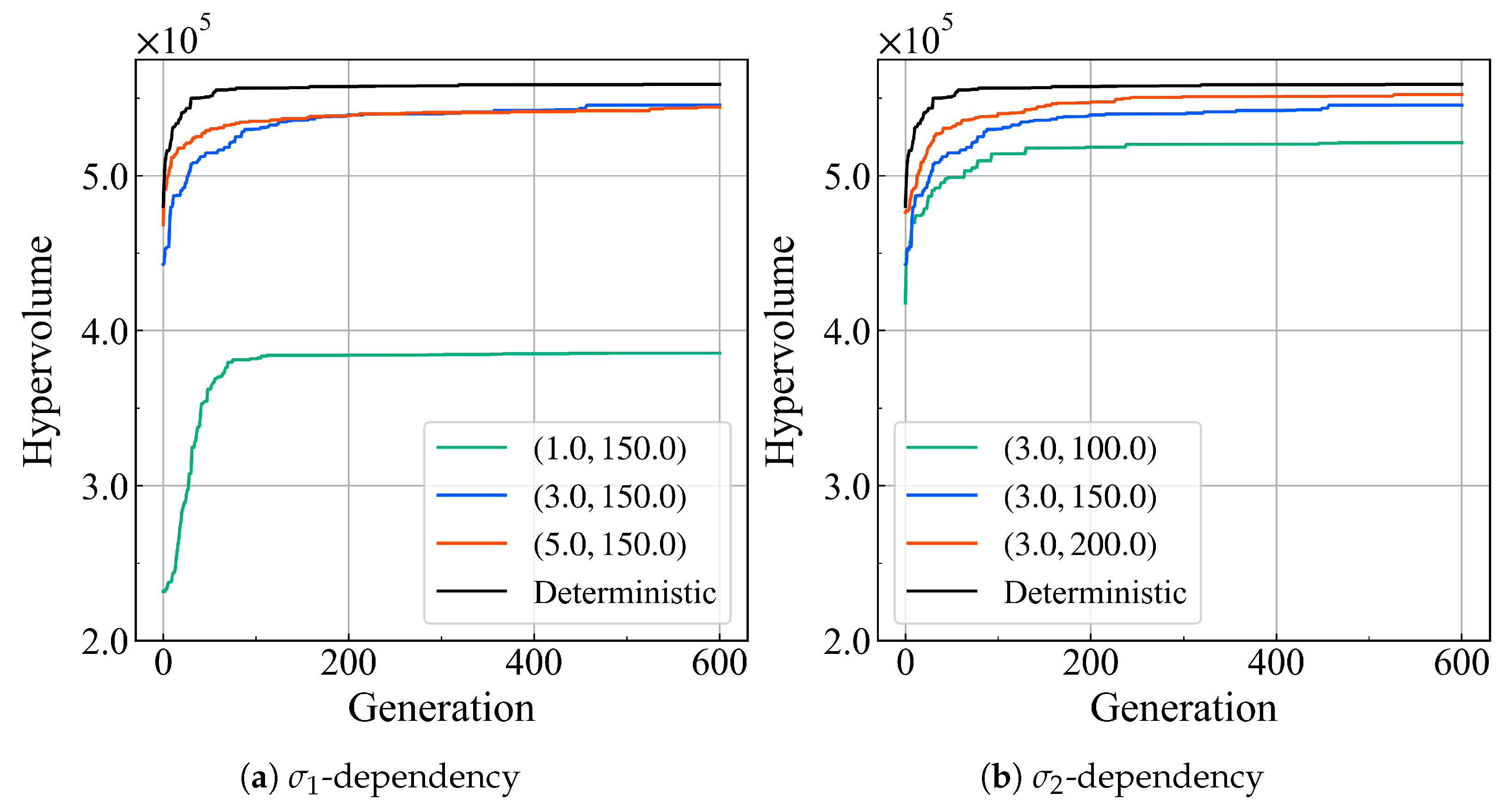
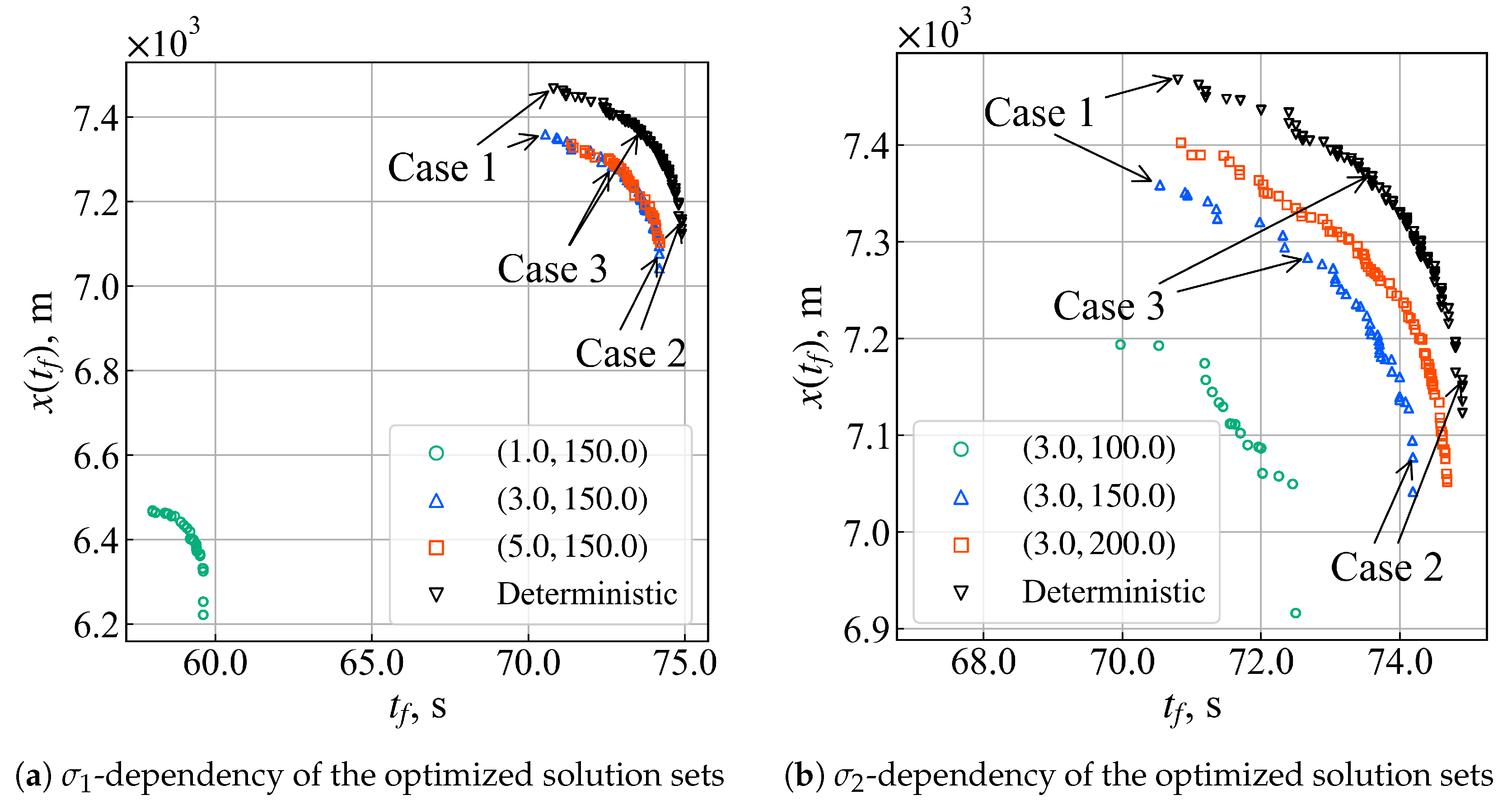
4.1. Non-Inferior Solutions Sets

In Figure 5, the sets of non-inferior solutions for each case of robustness parameters are presented. For the robust solution points, the plotted points indicate the weighted averages of the simulated objectives obtained via Equation (13). Therefore, each solution point of the deterministic problem contains a specific trajectory with the corresponding flight control history, while the solutions of the robust problem do not represent any realization of the trajectory. During the manipulation of either ${\sigma }_1$ or ${\sigma }_2$, the complementary value is maintained at its baseline: ${\sigma }_1=3.0$ and ${\sigma }_2=150.0$. The point solution sets (Case 1, Case 2, and Case 3) are the maximizer of the flight range, the maximizer of the flight time, and the representative compromised solution. The properties of the solutions are further assessed in the following subsection.

Non-dominated solutions obtained through deterministic optimization are superior to those obtained through robust optimization. A largest disparity was observed between the solution set of ${\sigma }_1=1.0$ and that of ${\sigma }_1=3.0$, as shown in Figure 5a. This represents a situation in which the overly constrained problem leads to the non-trivial solution set; simply, ${\sigma }_1=1.0$ is too conservative compared to the given uncertainty $\xi \in [-5,5]$ m/s, where the solution set is degraded considerably from that of ${\sigma }_1=3.0$. In contrast, the almost identical solution plots and hypervolumes were confirmed in the case of ${\sigma }_1=3.0$ and ${\sigma }_1=5.0$. This indicates that narrower standard deviation constraints (i.e., smaller ${\sigma }_1$ and ${\sigma }_2$) generally provide more conservative optimal solutions, although after being sufficiently relaxed, these values do not affect the objectives of the solution sets. A comparison with different values of ${\sigma }_1$ or ${\sigma }_2$ validates that the robust problem formulation allows us to seek the trade-space in the solution surface in a quantitative manner based on the different tolerance of the robustness.

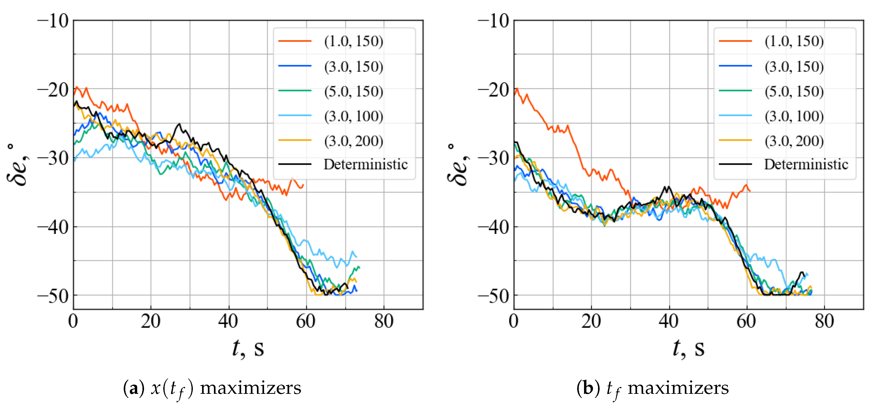
4.2. Comparisons of Representative Trajectories from Non-Inferior Solutions Set

This subsection examines the properties of the obtained guidance trajectories. First, the control histories of the representative point solutions in the non-inferior solution sets are presented in Figure 6. The controls that maximize $x\left(t_f\right)$ and $t_f$ for each set of $({\sigma }_1,{\sigma }_2)$ are illustrated. The robust control strategies depicted in the graph are concluded upon reaching the maximum time of flight among the trajectory ensembles. It is observed that the optimized control history exhibits a greater sensitivity to the selection of the primary objective to pursue, as opposed to the degree of robustness with which constraints are upheld in the presence of uncertainty. The only exception is the case of ${\sigma }_1=1.0$, in which the non-inferior solution set is significantly more conservative than the other cases, as shown in Figure 5.

Figure 7 illustrates the optimized trajectories corresponding to Case 1 (maximum flight range), Case 2 (maximum flight time), and Case 3 (compromised solution) point solutions shown in Figure 5. The deterministic case and baseline robust case $({\sigma }_1,{\sigma }_2=(3.0,150.0))$ are compared in each figure. Each robust solution is expressed in eight deterministic rollouts: six trajectories corresponding to the quadrature points, and two extreme scenarios (i.e., maximum headwind and tailwind).

In the final phase of the landing, all trajectories experience an increase in altitude. This climb in the nominal trajectories is much steeper than the rollouts of the robust solutions throughout the three point solutions shown in Figure 7. Furthermore, note that the nominal trajectories presented in Figure 7a,c nearly land on the ground at around $x=6000 \mathrm{m}$. Such control sequences lead to the early landing of the aircraft if it were to experience a strong headwind. On the contrary, the abrupt increase in altitude is mitigated in the trajectories sampled from the robust solutions due to the optimizer’s consideration of multiple EoMs, which ensures that early landings do not occur in any of these dynamics, particularly under conditions of worst wind uncertainty. Consideration of various contingencies is critical for the operation of the commercial aircraft landing [41], and this observation supports the importance of the newly obtained robust guidance.

Figure 8, Figure 9 and Figure 10 represent the other flight histories of the representative trajectories: the averages and standard deviations of the angle of attack, altitude, and the x and z components of the velocity. Note that the time-series data for each solution are terminated at the minimum time step among the trajectories sampled.

Because the control inputs of the robust and nominal solutions in Figure 6 are similar to each other, the histories of the angle of attack exhibit minimal variations. However, the changes in both $v_x$ and $v_z$ in the robust solutions are smaller than those of the deterministic solutions.

The control inputs are more sensitive to which objective to maximize rather than the uncertainty to be handled in the constraints, as shown in Figure 6. Although the difference in the flight time between the max. $x\left(t_f\right)$ solution (Case 1) and the max. $t_f$ solution (Case 2) is ∼4 s (approximately 5% of the entire flight time), a qualitative difference in the control policy and the realized trajectory is observed. First, the controller that maximizes the flight range monotonically decreases the elevator angle over the flight time, as shown in Figure 6a. On the contrary, Figure 6b indicates that $\delta e$ decreases quickly, and then experiences a slight increase before a sharp decrease near the landing to maximize the flight time. This corresponds to the trend of $\alpha$ that is depicted in Figure 8a and Figure 9a, where the maximum flight time control history has a larger angle of attack than that of the maximum flight distance solution by 2.5 deg. until the aircraft begins the final landing phase. Therefore, the trajectory with the maximum flight time experiences a larger lift force, which supports the aircraft to stay around $z=1000$ m at the beginning, as shown in Figure 9b compared to Figure 8b. This can also be validated from Figure 8d and Figure 9d, where the decrease in $v_z$ is delayed in the solution with the maximum flight time, whereas the solution with the maximum flight distance has a steeper drop in $v_z$ in the first 20 s. The high angle of attack also induces a larger drag force and slows down the aircraft in the x-direction, which can be confirmed via comparison with Figure 9c and Figure 8c. These factors contributed to extending the flight time of the solutions of Case 2, compared to those of Case 1. Finally, the intermediate characteristics in the flight profiles discussed above are observed in Figure 10, compared to Figure 8 and Figure 9.

4.3. Validation of the Robust Control Law

The optimized control histories from the baseline robust scenario (i.e., $({\sigma }_1,{\sigma }_2)=(3.0,150.0)$) are validated via an MC simulation using three representative trajectories. The standard deviations of the two objectives that are computed based on 10,000 rollouts of the MC simulation are presented in

Table 4. Standard deviations of the objectives obtained via MC simulations. The constraint values are set to $({\sigma }_1,{\sigma }_2)=(3.0,150.0)$ for the robust scenario.

Solution Points	Case	$\mathit{\mu }\left({\mathit{t}}_{\mathit{f}}\right)$	${\mathit{\sigma }}_1=\mathit{\sigma }\left({\mathit{t}}_{\mathit{f}}\right)$	$\mathit{\mu }\left(\mathit{x}\left({\mathit{t}}_{\mathit{f}}\right)\right)$	${\mathit{\sigma }}_2=\mathit{\sigma }\left(\mathit{x}\left({\mathit{t}}_{\mathit{f}}\right)\right)$
max. $x\left(t_f\right)$ (Case 1)	Determinisitc Robust	62.37 70.53	10.11 1.89	6720.98 7355.46	686.74 99.52
max. $t_f$ (Case 2)	Determinisitc Robust	72.07 74.08	6.693 1.80	6895.32 7081.88	402.39 102.98
Compromise (Case 3)	Determinisitc Robust	64.79 72.29	9.71 2.93	6610.21 7257.44	623.49 166.54

. We also generated trajectories based on the nominal solutions with the wind uncertainty and obtained the sensitivity of the nominal solution against the uncertainty. These values from the nominal solutions are important benchmarks to compare the performance of the robust solutions. The distributions of $t_f$ over the 1000 simulations are presented in Figure 11.

Table 4 confirms an increase in the averages of the objectives and a significant decrease in the standard deviation in the robust solutions, which proves the effectiveness of the robust formulation. The control sequences presented in Figure 6 look similar to each other when comparing the deterministic and robust solutions, although such a subtle difference in the control input critically changes the robustness of the flight control under the wind uncertainty. We can also visually confirm this from Figure 11, where the multimodal distributions in $t_f$ emerge for the deterministic solutions, which creates trajectories that have significantly less flight time. However, the distributions of $t_f$ for the robust solutions are mostly unimodal, which contributes to maintaining the small standard deviations.

Note that $\sigma \left(x\left(t_f\right)\right)$ for the robust solution in Case 3 ($\sigma \left(x\left(t_f\right)\right)=166.54$) infringes on the original constraint value of Equation (19l) ($\sigma \left(x\left(t_f\right)\right)\le {\sigma }_2=150.0$), although the reduction of the variance from the the deterministic solution is admitted. The factor that causes this problem is identified in Figure 11c, where some trajectories ended their flight around $t=60$ s. It is confirmed from Figure 7c that all six sky-blue trajectories corresponding to the quadrature points did not fail to reraise their altitude at the end of the flight; however, such an operation was not successful for the worst case shown in the purple trajectory, where the aircraft “crashed” on the ground. This reflects an inherent caveat of PCE that it can only consider the trajectories corresponding to the quadrature points. The stochastic parameters that are smaller (larger) than the minimum (maximum) quadrature points may still lead to the statistical constraints not being satisfied. This can be alleviated by the addition of more quadrature points for better approximation fidelity if the resilience to such a worst scenario must be addressed. Further investigation of approaches that prevent the destructive worst scenario at the edge cases while suppressing the number of quadrature points (i.e., computational cost) will be conducted in future studies. GPU parallelization [29] or multi-fidelity approaches, such as the efficient sparse grid quadrature method [11] and Kriging method [42], are expected to be suitable for the proposed method.

5. Conclusions

The landing operation of a supersonic aircraft that experiences a high angle of attack at a low speed is disturbed by meteorological factors, which affect its aerodynamic properties in a non-negligible manner. Therefore, this study presents the robust multi-objective optimal control of the CDO of the SST under wind uncertainty, based on the integration of non-intrusive PCE and a constrained MOEA. We allocate the constraints to three stages of the constraint-handling process (individual generation, trajectory ensemble, and evaluation by the MOEA), which allows us to implement various types of constraints while maintaining the formalism of robust multi-objective optimization.

The obtained robust solutions quantitatively show conservative non-inferior solution sets compared to the nominal solution sets. Multiple robust solutions with different constraint values show the trade-off between the tighter constraint values and the quality of the solutions. Such an investigation will be beneficial when searching for the pragmatic solution spaces for a new design concept of the SST. Furthermore, the validation via the MC simulation shows that the robust control sequences provide better objectives and smaller variances than the nominal solutions under uncertainty, which demonstrates the importance and effectiveness of the robust problem formulation.

References

1. Ericsson, L.E. Pitch rate effects on delta wing vortex breakdown. J. Aircr. 1996, 33, 639–642. [Google Scholar] [CrossRef]
2. Razak, K.; Snyder, M., Jr. A Review of the Planform Effects on the Low-Speed Aerodynamic Characteristics of Triangular and Modified Triangular Wings; Technical Report; NASA: Cleveland, OH, USA, 1966. [Google Scholar]
3. Pourtakdoust, S.H.; Kiani, M.; Hassanpour, A. Optimal trajectory planning for flight through microburst wind shears. Aerosp. Sci. Technol. 2011, 15, 567–576. [Google Scholar] [CrossRef]
4. Lymperopoulos, I.; Lygeros, J. Sequential Monte Carlo methods for multi-aircraft trajectory prediction in air traffic management. Int. J. Adapt. Control Signal Process. 2010, 24, 830–849. [Google Scholar] [CrossRef]
5. Lecchini Visintini, A.; Glover, W.; Lygeros, J.; Maciejowski, J. Monte Carlo Optimization for Conflict Resolution in Air Traffic Control. IEEE Trans. Intell. Transp. Syst. 2006, 7, 470–482. [Google Scholar] [CrossRef]
6. Markley, F.L.; Carpenter, J.R. Generalized linear covariance analysis. J. Astronaut. Sci. 2009, 57, 233–260. [Google Scholar] [CrossRef]
7. Geller, D. Linear Covariance Techniques for Orbital Rendezvous Analysis and Autonomous Onboard Mission Planning. J. Guid. Control. Dyn. 2006, 29, 1404–1414. [Google Scholar] [CrossRef]
8. Saunders, B. Optimal Trajectory Design under Uncertainty. Master’s Thesis, Department of Aeronautics and Astronautics, MIT, Cambridge, MA, USA, 2012. [Google Scholar]
9. Tang, G.; Luo, Y.; Li, H. Optimal robust linearized impulsive rendezvous, Aerospace Science Technology. Aerosp. Sci. Technol. 2007, 11, 314–325. [Google Scholar] [CrossRef]
10. Xiu, D.; Karniadakis, G. The Wiener-Askey Polynomial Chaos for Stochastic Differential Equations. SIAM J. Sci. Comput. 2002, 60, 897–936. [Google Scholar] [CrossRef]
11. Eldred, M.; Webster, C.; Constantine, P. Evaluation of Non-Intrusive Approaches for Wiener-Askey Generalized Polynomial Chaos. In Proceedings of the 49th AIAA/ASME/ASCE/AHS/ASC Structures, Structural Dynamics, and Materials Conference, Schaumburg, IL, USA, 7–10 April 2008; AIAA: Reston, VA, USA, 2008. [Google Scholar] [CrossRef]
12. Li, X.; Nair, P.; Zhang, Z.; Gao, L.; Gao, C. Aircraft Robust Trajectory Optimization Using Nonintrusive Polynomial Chaos. J. Aircr. 2014, 51, 1592–1603. [Google Scholar] [CrossRef]
13. Matsuno, Y.; Tsuchiya, T.; Wei, J.; Hwang, I.; Matayoshi, N. Stochastic optimal control for aircraft conflict resolution under wind uncertainty. Neural Comput. Appl. 2015, 43, 77–88. [Google Scholar] [CrossRef]
14. Fisher, J.; Bhattacharya, R. Optimal trajectory generation with probabilistic system uncertainty using polynomial chaos. J. Dyn. Syst. Meas. Control 2011, 133, 014501. [Google Scholar] [CrossRef]
15. Xiong, F.; Xiong, Y.; Xue, B. Trajectory Optimization under Uncertainty based on Polynomial Chaos Expansion. In Proceedings of the AIAA Guidance, Navigation, and Control Conference, Kissimmee, FL, USA, 5–9 January 2015; AIAA: Reston, VA, USA, 2015; p. 1761. [Google Scholar] [CrossRef]
16. Casado, E.; Civita, M.L.; Vilaplana, M.; McGookin, E.W. Quantification of aircraft trajectory prediction uncertainty using polynomial chaos expansions. In Proceedings of the 2017 IEEE/AIAA 36th Digital Avionics Systems Conference (DASC), St. Petersburg, FL, USA, 17–21 September 2017; pp. 1–11. [Google Scholar] [CrossRef]
17. Wang, F.; Yang, S.; Xiong, F.; Lin, Q.; Song, J. Robust trajectory optimization using polynomial chaos and convex optimization. Aerosp. Sci. Technol. 2019, 92, 314–325. [Google Scholar] [CrossRef]
18. Nakka, Y.K.; Chung, S. Trajectory optimization for chance-constrained nonlinear stochastic systems. In Proceedings of the 2019 IEEE 58th Conference on Decision and Control, Nice, France, 11–13 December 2019; IEEE: New York, NY, USA, 2019; pp. 3811–3818. [Google Scholar] [CrossRef]
19. Gambier, A.; Badreddin, E. Multi-objective Optimal Control: An Overview. In Proceedings of the 2007 IEEE International Conference on Control Applications, Singapore, 1–3 October 2007; pp. 170–175. [Google Scholar] [CrossRef]
20. Mueller, R. Multi-Objective Optimization of an Aircraft Trajectory between Cities using an Inverse Model Approach. In Proceedings of the AIAA Modeling and Simulation Technologies Conference, Minneapolis, MN, USA, 13–16 August 2012; p. 4489. [Google Scholar]
21. Hartjes, S.; Visser, H. Efficient trajectory parameterization for environmental optimization of departure flight paths using a genetic algorithm. Proc. Inst. Mech. Eng. Part G J. Aerosp. Eng. 2017, 231, 1115–1123. [Google Scholar] [CrossRef]
22. Ho-Huu, V.; Hartjes, S.; Geijselaers, L.; Visser, H.; Curran, R. Optimization of noise abatement aircraft terminal routes using a multi-objective evolutionary algorithm based on decomposition. Transp. Res. Procedia 2018, 29, 157–168. [Google Scholar] [CrossRef]
23. Kanazaki, M.; Othman, N.B. Time-series optimization methodology and knowledge discovery of descend trajectory for civil aircraft. In Proceedings of the 2016 IEEE Congress on Evolutionary Computation (CEC), Vancouver, BC, Canada, 24–29 July 2016; IEEE: New York, NY, USA, 2016; pp. 893–900. [Google Scholar]
24. Kanazaki, M.; Setoguchi, N.; Saisyo, R. Evolutionary Algorithm Applied to Time-Series Landing Flight Path and Control Optimization of Supersonic Transport. Neural Comput. Appl. 2021, 35, 1211–1223. [Google Scholar] [CrossRef]
25. Marto, S.; Vasile, M. Many-Objective Robust Trajectory Optimisation Under Epistemic Uncertainty and Imprecision. Acta Astronaut. 2022, 191, 99–124. [Google Scholar] [CrossRef]
26. Luo, Y.; Tang, G.; Lei, Y. Optimal Multi-Objective Linearized Impulsive Rendezvous. J. Guid. Control. Dyn. 2007, 30, 383–389. [Google Scholar] [CrossRef]
27. Luo, Y.; Yang, Z.; Li, H. Robust optimization of nonlinear impulsive rendezvous with uncertainty. Sci. China Phys. Mech. Astron. 2014, 57, 731–740. [Google Scholar] [CrossRef]
28. Yang, Z.; Luo, Y.z.; Zhang, J. Robust Planning of Nonlinear Rendezvous with Uncertainty. J. Guid. Control. Dyn. 2017, 40, 1954–1967. [Google Scholar] [CrossRef]
29. González-Arribas, D.; Sanjurjo-Rivo, M.; Soler, M. Multiobjective Optimisation of Aircraft Trajectories Under Wind Uncertainty Using GPU Parallelism and Genetic Algorithms. In Evolutionary and Deterministic Methods for Design Optimization and Control with Applications to Industrial and Societal Problems; Andrés-Pérez, E., González, L., Periaux, J., Gauger, N., Quagliarella, D., Giannakoglou, K., Eds.; Springer: Cham, Switzerland, 2019; pp. 453–466. [Google Scholar]
30. Levine, J.; Blaney, D.; Connemey, J.; Greeley, R.; Head III, J.; Hoffman, J.; Jakosky, B.; McKay, C.; Sotin, C.; Summers, M. Science from a Mars airplane: The aerial regional-scale environmental survey (ARES) of Mars. In Proceedings of the 2nd AIAA “Unmanned Unlimited” Conf. and Workshop & Exhibit, San Diego, CA, USA, 15–18 September 2003; p. 6576. [Google Scholar]
31. Hall, J.L.; Cameron, J.; Pauken, M.; Izraelevitz, J.; Dominguez, M.W.; Wehage, K.T. Altitude-controlled light gas balloons for Venus and Titan exploration. In Proceedings of the AIAA Aviation 2019 Forum, Dallas, TX, USA, 17–21 June 2019; p. 3194. [Google Scholar]
32. Toyoda, T.; Kanazaki, M. Trajectory Optimization for Space Debris Re-entry Considering Land Security by Evolutionary Algorithm. In Proceedings of the 34th International Symposium on Space Technology and Science (ISTS), Fukuoka, Japan, 3–9 June 2023. [Google Scholar]
33. Takubo, Y.; Kanazaki, M. Robust Constrained Multi-objective Evolutionary Algorithm based on Polynomial Chaos Expansion for Trajectory Optimization. In Proceedings of the 2022 IEEE Congress on Evolutionary Computation (CEC), Padua, Italy, 18–23 July 2022; IEEE: New York, NY, USA, 2022; pp. 1–9. [Google Scholar]
34. Bryson, A.E. Applied Optimal Control: Optimization, Estimation, and Control; Routledge: Milton Park, UK, 2018. [Google Scholar]
35. González-Arribas, D.; Soler, M.; Sanjurjo-Rivo, M. Robust Aircraft Trajectory Planning Under Wind Uncertainty Using Optimal Control. J. Guid. Control. Dyn. 2018, 41, 673–688. [Google Scholar] [CrossRef]
36. Mühlpfordt, T.; Roald, L.; Hagenmeyer, V.; Faulwasser, T.; Misra, S. Chance-Constrained AC Optimal Power Flow: A Polynomial Chaos Approach. IEEE Trans. Power Syst. 2019, 34, 4806–4816. [Google Scholar] [CrossRef]
37. Deb, K. An efficient constraint handling method for genetic algorithms. Comput. Methods Appl. Mech. Eng. 2000, 186, 311–338. [Google Scholar] [CrossRef]
38. Coello, C.A.C. Theoretical and numerical constraint-handling techniques used with evolutionary algorithms: A survey of the state of the art. Comput. Methods Appl. Mech. Eng. 2002, 191, 1245–1287. [Google Scholar] [CrossRef]
39. Kwak, D.; Miyata, K.; Noguchi, M.; Sunada, Y.; Rinoie, K. Experimental investigation of high lift device for SST. In The National Aerospace Laboratory Technical Report; NAL TR-1450; National Aerospace Laboratory(NAL): Tokyo, Japan, 2002. (In Japanese) [Google Scholar]
40. Jones, D.R.; Schonlau, M.; Welch, W.J. Efficient global optimization of expensive black-box functions. J. Glob. Optim. 1988, 13, 455–492. [Google Scholar] [CrossRef]
41. Code of Federal Regulations, Title 14, Part 121.195. 2023. Available online: https://www.ecfr.gov/current/title-14/chapter-I/subchapter-G/part-121 (accessed on 24 October 2023).
42. Matsuno, Y.; Tsuchiya, T.; Matayoshi, N. Near-Optimal Control for Aircraft Conflict Resolution in the Presence of Uncertainty. J. Guid. Control. Dyn. 2016, 39, 326–338. [Google Scholar] [CrossRef]
Figure 1. Process of constraint-handling by embedding trajectory ensemble into the EA.
Aerospace 10 00929 g001
Figure 2. Airframe of the SST model [24]. The optimization variables are the time variation of δ e .
Aerospace 10 00929 g002
Figure 3. Allocation of the constraints for the deterministic problem in Equation (15) and robust problem in Equation (20).
Aerospace 10 00929 g003
Figure 4. Results of multi-objective optimization problems: history of hypervolume. The values in the legends represent ( σ 1 , σ 2 ) = ( σ ( t f ) ) , σ ( x ( t f ) ) .
Aerospace 10 00929 g004
Figure 5. Noninferiror solution sets for different stochastic scenarios. The values in the legends represent ( σ 1 , σ 2 ) = ( σ ( t f ) ) , σ ( x ( t f ) ) .
Aerospace 10 00929 g005
Figure 6. Comparison of the control sequences at each problem scenario. The values in legends represent ( σ 1 , σ 2 ) = ( σ ( t f ) ) , σ ( x ( t f ) ) .
Aerospace 10 00929 g006
Figure 7. Comparison of the nominal and baseline robust trajectories. The nominal (deterministic) trajectories are presented in orange, the generated trajectories corresponding to the quadrature points are in sky-blue, and the trajectories with the maximum tailwind and headwind scenarios are in purple and blue, respectively, with dotted patterns.
Aerospace 10 00929 g007
Figure 8. Comparisonof the flight properties of the nominal and robust trajectories ( σ 1 , σ 2 ) = ( 3.0 , 150.0 ) (max. x ( t f ) , Case 1). The nominal trajectory and the average of the robust trajectories are presented in orange and blue, respectively. The sky-blue range shows the ± σ variance.
Aerospace 10 00929 g008
Figure 9. Comparison of the flight properties of the nominal and robust trajectories ( σ 1 , σ 2 ) = ( 3.0 , 150.0 ) (max. t f , Case 2). The nominal trajectory and the average of the robust trajectories are presented in orange and blue, respectively. The sky-blue range shows the ± σ variance.
Aerospace 10 00929 g009
Figure 10. Comparison of the flight properties of the nominal and robust trajectories ( σ 1 , σ 2 ) = ( 3.0 , 150.0 ) (compromised solution, Case 3). The nominal trajectory and the average of the robust trajectories are presented in orange and blue, respectively. The sky-blue range shows the ± σ variance.
Aerospace 10 00929 g010
Figure 11. Distribution of the flight time of the 1000 MC simulations.
Aerospace 10 00929 g011