2. The Use of the Magnetic Field of the Earth as a Direction Reference
TN, also known as geographic North or geodetic North, refers to the direction along the Earth’s surface towards the North Pole. It is the fixed point where the Earth’s axis of rotation intersects the Earth’s surface in the Northern Hemisphere. TN serves as a natural reference point for navigation, as it remains constant and is not influenced by the Earth’s magnetic field. Historically, TN as determined from observations of the night sky was the main reference used by ancient civilisations to navigate.
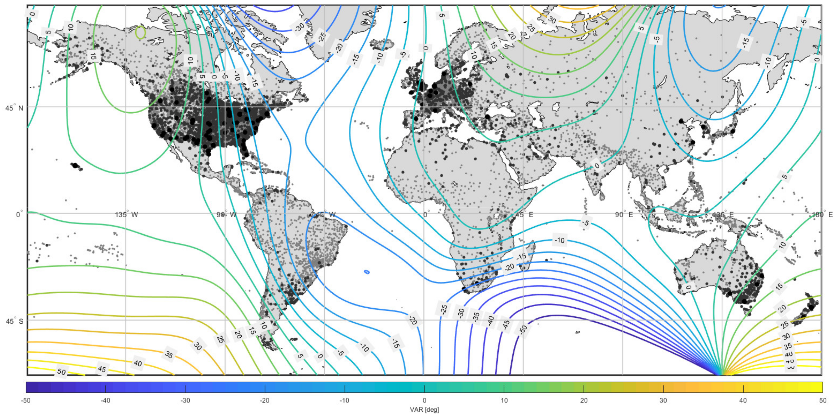
In contrast to TN, MN is the direction towards which a compass needle points under the influence of the Earth’s magnetic field. The location of the Magnetic North Pole is not fixed and has been gradually shifting over time due to changes in the Earth’s magnetic field. This movement results in magnetic declination or variation (VAR), which is the angle between MN and TN at a given location at a certain date (
Figure 1 and
Figure 2). Navigators must account for VAR when using a compass to determine their bearings with respect to the meridian. The variation was discovered five centuries ago by Cristopher Columbus during his historic exploration of the Big Ocean by way of contrasting compass indications and astronomic observations.
Magnetic North was taken as the reference at the beginning of aviation, in the early 1900s, due to the low cost of a sensor and despite the many inconveniences which are presented further. A magnetic compass is inexpensive (any magnetised iron mobile object). A sensor for True North was not available until much later (except for Astrocompasses, which are not practical in air navigation). The development of inertial navigation technology (INS/IRS) in the 1960s and the global navigation satellite technology (GNSS) in the 1990s enabled the measurement or the estimate of the TN reference, but they were very expensive initially. The MN reference was maintained as a common reference to all segments of aviation as it is the cost-effective common denominator reference. For Air Traffic Management, it is essential that all flights share the same reference, from the best equipped airliner to the basically equipped general aviation airplane or helicopter. Therefore, it was a forced choice at the beginning. However, this balance has changed since the relative cost of different navigation technologies has evolved. Currently, it is equally expensive to measure MN and TN on board an aircraft, and even UAVs benefit from true reference from the inexpensive GNSS receivers they use. Therefore, there was a cost-effectiveness rationale for the MN choice, which no longer exists.
The MN replacement by TN is a change in reference problem. Everything is the same (mathematical models, algorithms, software), except the zero setting, which is changed or offset.
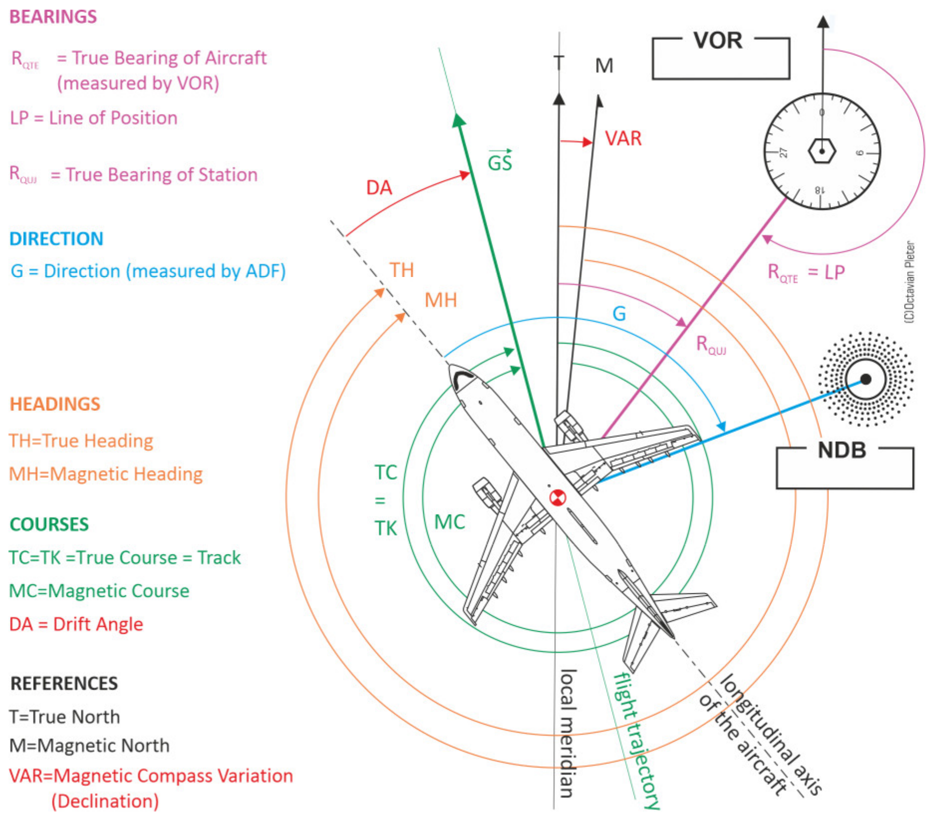
Figure 2 represents the azimuths currently used in horizontal air navigation, and
Figure 3 demonstrates the situation after the transition.
The advantage of the instrumentation cost effectiveness shifted from MN instruments (compasses) to TN instruments (GNSS). Gyro directional instruments are reference neutral because they use the gyroscope rigidity effect, which maintains a direction with respect to a distant star, which is neither the MN nor TN reference. Therefore, the gyro directional instruments require adjustments from time to time to correct their reference. Currently, this is performed for MN, but this could easily be changed with the use of a TN GNSS sensor instead of a magnetometer (flux valve).
The accuracy expected from the on-board legacy magnetic compass is remarkably low: ±10° even for the best equipped airliners (e.g., FAR 25.1327 or CS 25.1327 specifications for large aeroplanes). In reality, the instruments frequently deliver a much better accuracy, but this low expectation of accuracy is indicative of the limited reliability and of the technical hurdles arising from the need to sense the magnetic field of the Earth on board an aircraft. The accuracy factor is decisively on the TN side. GNSS sensors deliver the azimuth reference with at least two orders of magnitude more accuracy than the magnetic sensors, and this does not come from the technology of the sensor itself, but more from the fact that the aircraft in which the sensor is installed is a major magnetic field perturbator itself. These perturbations are changing in time, and reflect the local magnetic fields induced by the on-board power lines (depending on the electric current) and by transmitter antennas which produce electromagnetic fields. Since there is much uncertainty in the power lines usage and transmitter antennas usage, magnetic compasses always only deliver an approximate azimuth. On-board magnetic sensors (compasses, flux valves) are subject to many factors of deviation and errors, requiring a costly process of calibration and correction (compass swinging).
On top of those sources of inaccuracy, when the magnetic direction is converted to true (as it should be for any navigation calculations), there is another source of errors introduced by the value of magnetic compass variation (VAR) in use. VAR is variable in space and time, and it is usually given approximately. It is taken to be the same for a certain region and for a certain time interval. These approximations are an additional and separate source of errors.
North of latitudes 75° N and South of latitudes 63° S, aviation is already operating in TN. For example, TN air navigation has always been operational in Northern Canada.
3. Irregularity, Unpredictability, and Uncertainties of the Magnetic Field of the Earth
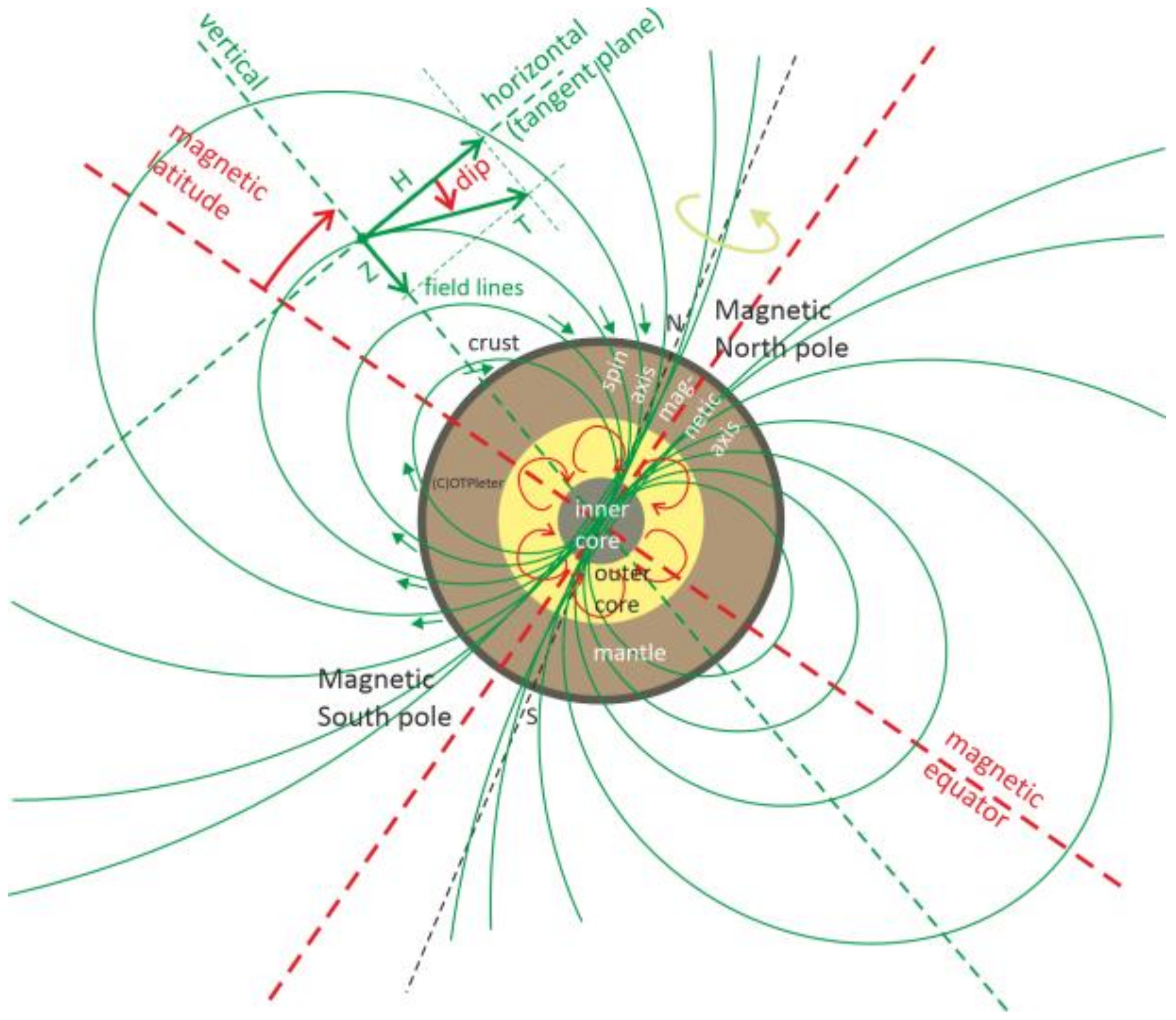
The magnetic compass measures the direction of the horizontal component of the magnetic field of the Earth, H, in
Figure 4. This field is generated by convective flow of the Earth’s liquid outer core. The intensity of the magnetic field, T, has a horizontal and a vertical component (H and Z).
The vertical component, Z, is sensed and used only by animals to navigate (providing a magnetic latitude sensing), but in air navigation it creates problems because it stands in the way of an accurate measurement of the useful horizontal component. Magnetic compasses in aviation have a specific vulnerability to the longitudinal and lateral accelerations. Both direct indicating magnetic compass and flux valves/magnetometers are measuring the horizontal component of the magnetic field. To separate the horizontal component from the vertical component, a pendulum mount is used to sense the apparent gravity vertical (plumb bob). This solution is adequate for boats and ships to compensate for pitch and bank angles, in absence of significant persistent longitudinal and lateral accelerations. However, aircraft are subject to such accelerations of large amplitude, which deviate the pendulum and cause sizeable magnetic compass errors. Not only do the vertical component of the magnetic field distorts the indication, but also the hard and soft iron components of the aircraft on the Z axis come into play. As the magnetic compass calibration (compass swinging) is performed on a horizontal platform, these components are never measured and compensated. Even the most sophisticated sensors such as 3D magnetometers, where the horizontal component is extracted from the 3D magnetic field line by computing, are affected by the Z axis hard and soft iron components. These sensors could be perfect in the laboratory, but once installed in an aircraft, they deviate. The magnetic direction sensors in aviation are admitted to be the least accurate, with a staggering tolerance as mentioned below, in spite of the fact that their calibration process is one of the most complex and expensive among all other sensors.
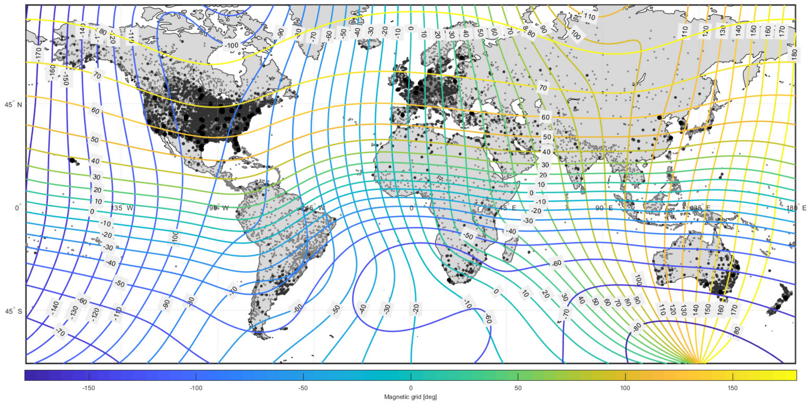
The best location for the measurement of H is the magnetic equator, where Z is zero (
Figure 5). However, when the magnetic latitude is large (and consequently the dip angle), Z supersedes H, making it hard to accurately measure the MN. That is why ICAO does not allow the usage of MN reference above 75° N latitude (and 63° S). Therefore, in the polar regions, TN is the direction reference.
The magnetic field of the Earth is unpredictable, and this is the least one expects from a general reference. The following factors define the uncertainties of the magnetic field of the Earth:
It is variable in space and time, and, in principle, it is nowcasted, requiring costly updates to maintain the nowcast model accurate; space variability is represented by the isogonal model (
Figure 1) and by the magnetic grid world map (
Figure 5). The variability and consequently the irregularity of the magnetic field in space has three main causes:
There are no methods to forecast the changes in the magnetic field of the Earth other than extrapolating past observations. There has been a significant increase in the rate of change in the past decades, and this increase was not predicted; at present, science does not provide models of the Earth’s magnetic field which could be used to forecast such accelerations; air navigation copes well with the rate of change in the magnetic field, but less so with the accelerations of change, such as the one illustrated by the fourfold increase in the Magnetic North Pole wander speed, explained further in Figure 10.
The magnetic field of the Earth has weakened by 20% over the last two centuries and its evolution cannot be predicted. Magnetic pole reversal or tentative reversal may not be ruled out, as presented further; such unpredictable, yet expected, catastrophic events would deny the use of the magnetic field for navigation altogether.
Magnetic thunderstorms are local disturbances of the magnetic field which are not predictable and significantly impact the magnetic sensors in affected areas.
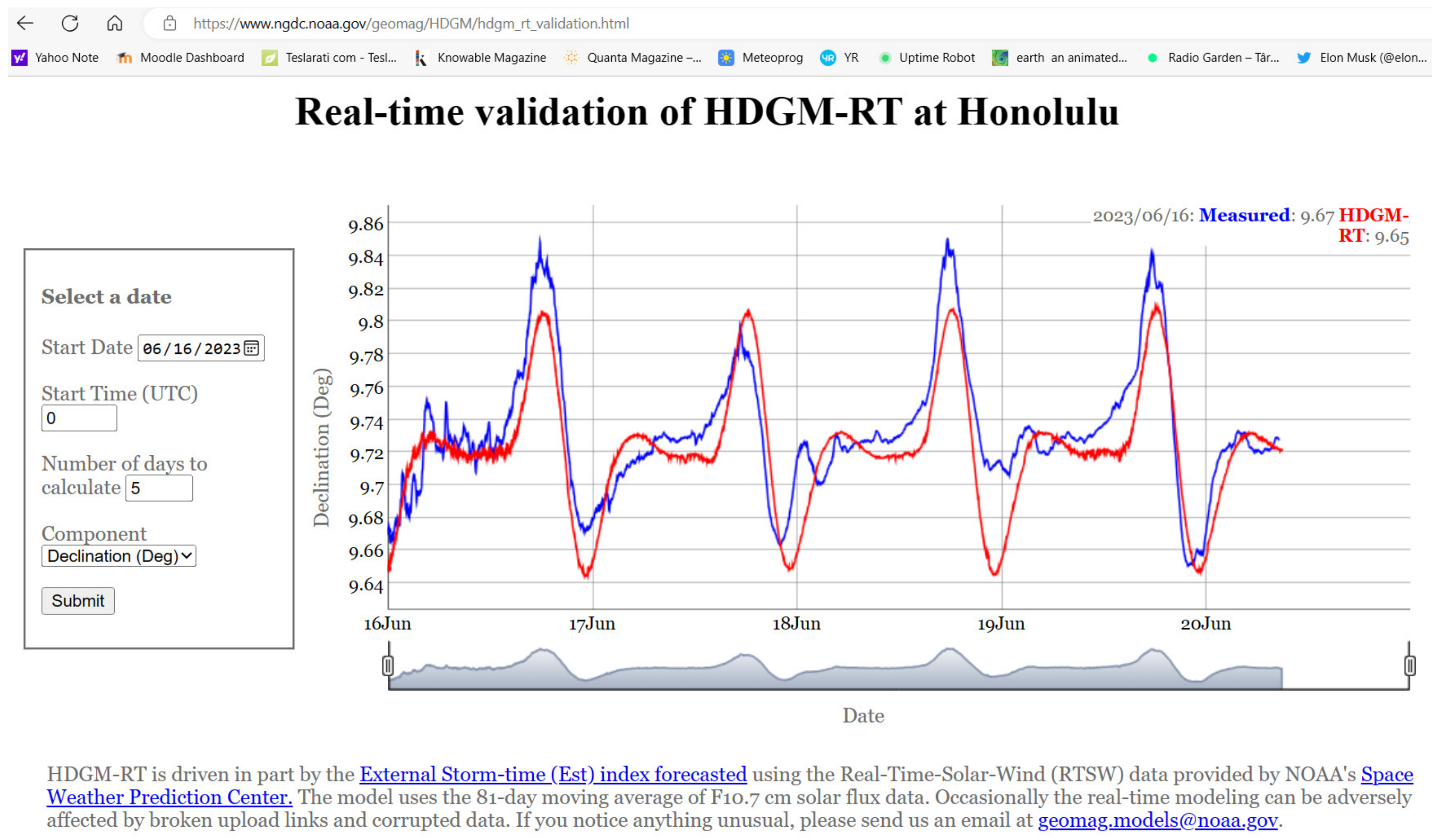
There is a daily variability of VAR of the order of half a degree, as illustrated by
Figure 6. In air navigation, this variability is operationally ignored because it is absorbed in the magnetic compass error margin. However, this fact is one more reason for the low accuracy of magnetic sensing.
The polarity of the magnetic field is not constant and various scientific methods such as those using ice deposits and river sediments of iron minerals revealed that in the Earth’s history there were many pole reversals and also tentative reversals, which represent catastrophic events for navigation in case MN is not replaced by the time of such a change; even with a low probability, such an event might unfold in the near future, requiring a contingency plan from aviation decision makers.
The irregularity of the magnetic field of the Earth is obvious in
Figure 5, which represents the current magnetic frame of the world together with the magnetic latitudes and longitudes. The Mercator projection represents the geodetic latitude and longitude lines as horizontal and vertical straight lines, respectively. The irregularity of the magnetic frame compels all the air navigation methods to be dependent on True North instead, which offers a regular grid, with equidistant horizontal parallels and perpendicular equidistant meridians.
The variability in time of the Earth’s magnetic field may be classified in time scale categories as presented in
Table 1 and
Table 2.
Magnetic thunderstorms are frequent in some parts of the world, such as the region in the Atlantic known as the Bermuda Triangle, but their impact on aviation is very small, especially since satellite navigation provided an alternative method of oceanic air navigation. However, this represents a waiver of the Magnetic North rules.
Episodic variations are illustrated by the example in
Figure 6. Although their amplitude is small (typically 0.2° per day), they put a limit on the accuracy required from magnetic compasses and sensors.
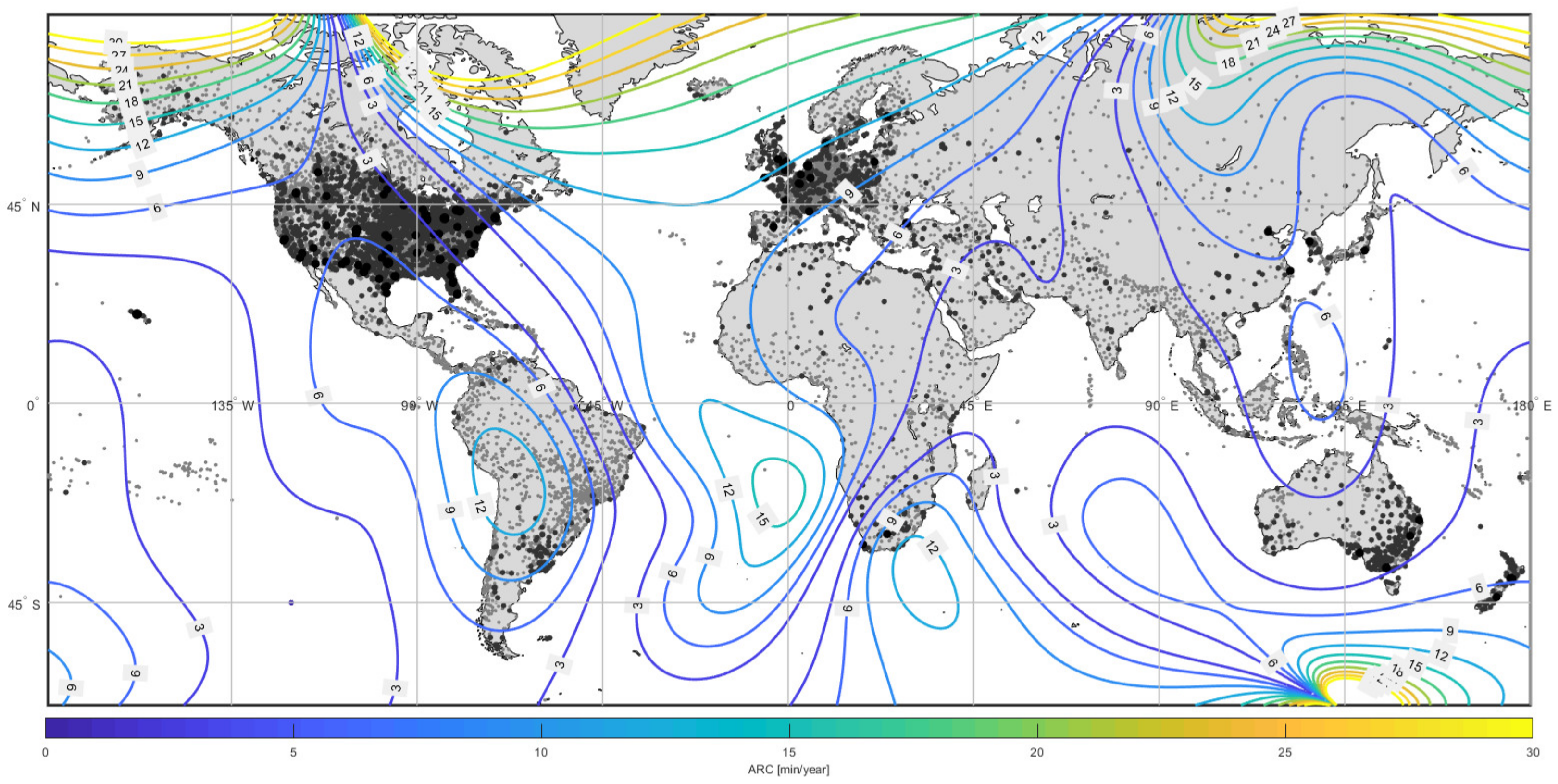
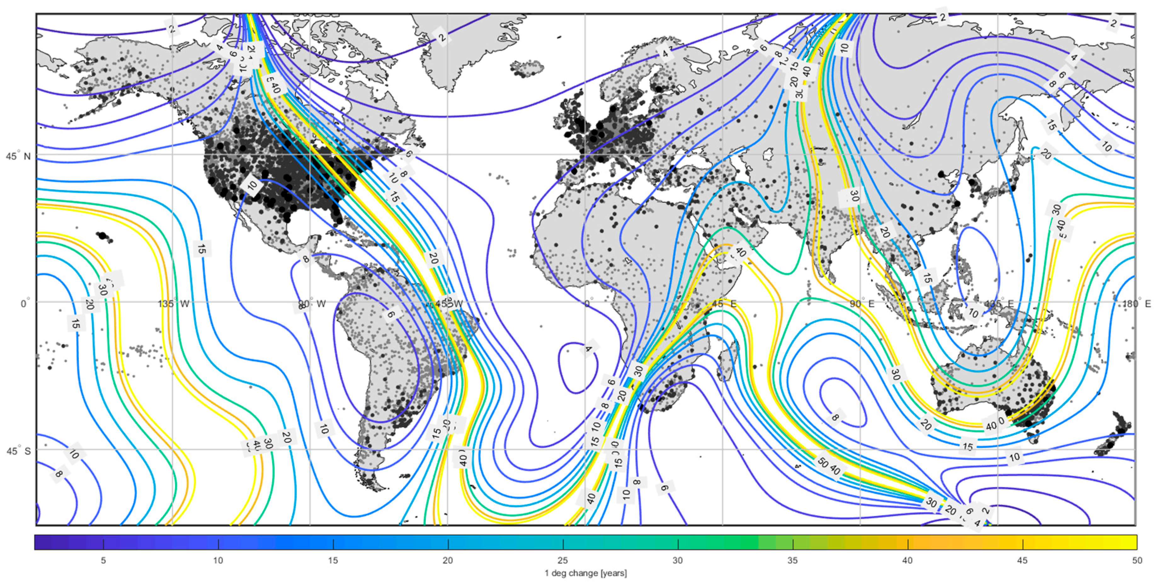
The annual variability of the magnetic variation in air navigation is expressed as the Annual Rate of Change (ARC) of VAR, in minutes of arc, West or East.
Figure 7 represents the ARC isogradient curves without sign (in absolute value) to serve the purpose of illustrating just the amplitude of the VAR rate. To serve the practical purposes of air navigation, ARC is considered constant, but this is an approximation of the reality. In some parts of the world, the ARC is changing itself over the years, and this could be expressed as a second-order ARC. The situation in
Figure 7 corresponds to the year 2023, but in 2033 it could be slightly different. There is, however, no forecasting method for these slight changes.
The secular variability is illustrated in
Figure 8 and represents the wander of the magnetic poles. In the polar regions, the secular variability causes the annual changes to be very large and unpredictable. However, these regions are outside the 75° N 63° S magnetic navigation range, and TN is used instead.
Regarding the millennial variability, it was considered irrelevant to practical air navigation due to its time scale. However, it has been better understood just recently [
5]. It consists of reversals of the magnetic poles of the Earth after a number of millennia, so its impact would be catastrophic on the use of the MN reference.
The recent advances in the study of the geomagnetic history allowed the scientific community understanding of the fact that magnetic pole reversals (Chrons) are just the extreme manifestation of the millennial variation, which otherwise consists of unsuccessful tentative reversals (Subchrons). The stability of the magnetic poles has two states (N-S and S-N configurations), but the flip-flop between these two states is not sudden and there are unstable intermediary states. If the millennial variation reaches a tipping point, the poles become reversed. If not, the poles revert back to their initial hemisphere, but the disturbance is still major to whomsoever attempts to use MN as a reference. We call this a tentative reversal, or Subchron, as it is called by the geomagnetic scientists. Also, there are unstable situations called Cryptochrons, when a tentative reversal takes a long time and the wander of the magnetic poles becomes very complex, including a situation when both magnetic poles float on the same side of the equator [
8] (see
Figure 9). For example, the most recent Cryptochron occurred between 493,000 and 504,000 years ago. In the 9000-year time interval, both poles went to the Equator, and at certain moments in time they were even in the same hemisphere [
9].
The Matuyama–Brunhes (M–B) polarity transition occurred approximately 780,000 years ago, marking the transition from the Matuyama reversed polarity Chron to the Brunhes normal polarity Chron. Some studies suggest that this reversal happened relatively quickly, within hundreds to a few thousand years, which is considered rapid in geological terms [
10].
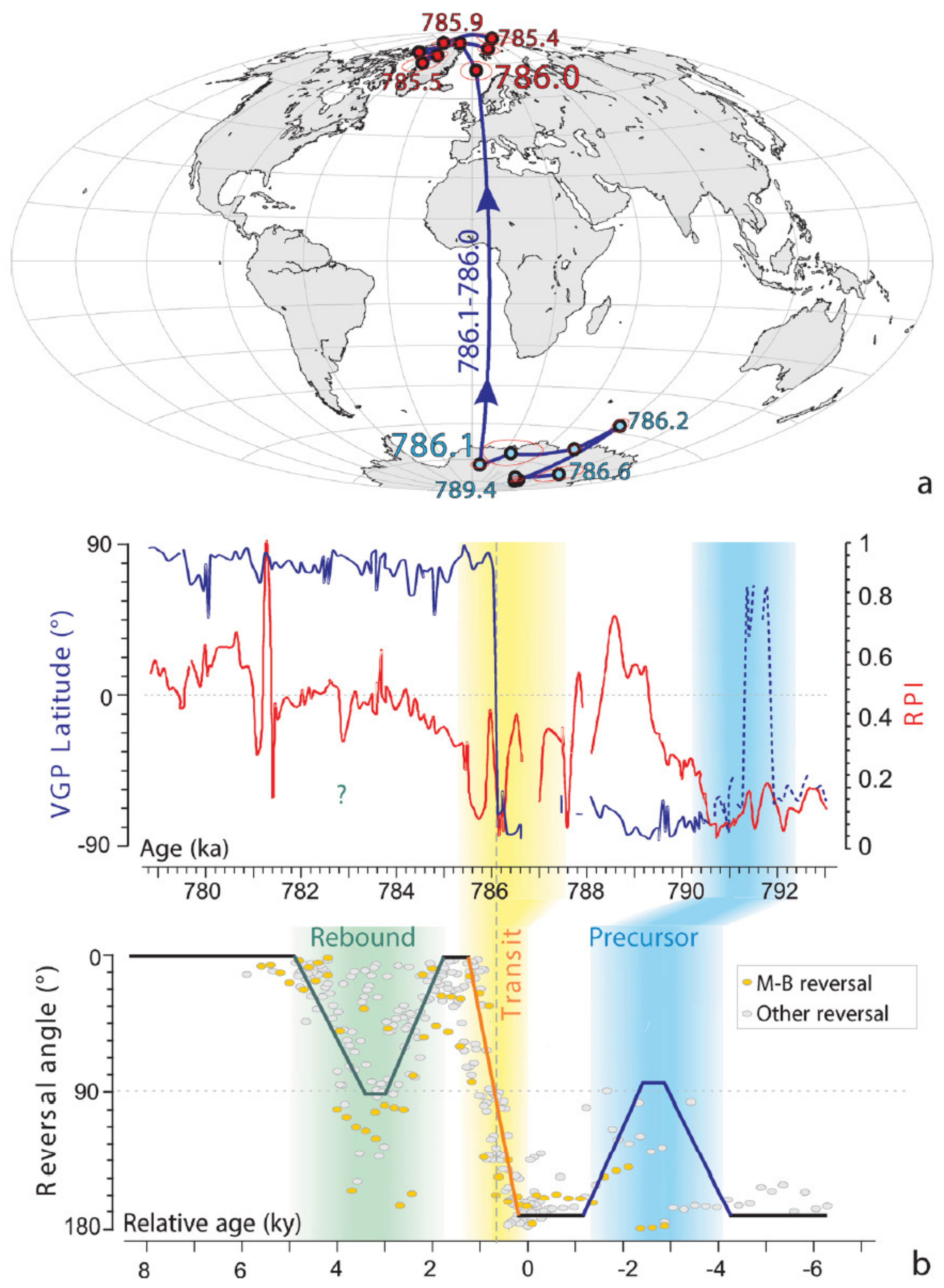
Figure 8.
(
a) Virtual geomagnetic pole (VGP) path reconstructed for the palaeomagnetic data from the discrete specimens around the M−B transition in the Horseshoe section. (
b) Stratigraphic trends for the VGP latitude (blue curve) and RPI scaled to unit maximum (red curve) for the Horseshoe section compared with the schematic reversal path of [
11], from compilation of reversal records in data flows, illustrating the succession of the reversal precursor, polarity switch and rebound. Coloured area in the Horseshoe plot indicates the stratigraphic intervals of minimum RPI that have been correlated with the precursor and the transit phases of the [
11] scheme. Time units are kilo-years, which correspond to 1000 years, so the reversal took 100 years (from 786.1 until 786.0 ky).
Comparatively, the earlier reversal events, such as the Olduvai Subchron and the Cobb Mountain event, show significant differences in terms of duration and the behaviour of the Earth’s magnetic field during the reversal process. For example, the Olduvai Subchron, which occurred around 1.95 million years ago, is characterized by a normal polarity interval that lasted about 50,000 years within the Matuyama reversed polarity Chron [
12]. The Cobb Mountain event, which took place around 1.2 million years ago, is marked by a very short normal polarity interval lasting only a few thousand years. As demonstrated in [
10], the last full reversal required just 100 years (
Figure 8). This is a relevant finding in the context of air navigation as discussed further.
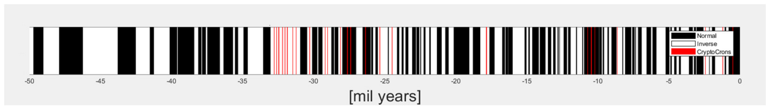
Figure 9.
The magnetic pole reversals (Chrons) in the past 50 mil years are the intervals between black and white, with black representing the present-day polarity. Cryptochron or Subchron periods represented in red; the polarity was not clear. Authors’ diagram using data from [
8].
Figure 9.
The magnetic pole reversals (Chrons) in the past 50 mil years are the intervals between black and white, with black representing the present-day polarity. Cryptochron or Subchron periods represented in red; the polarity was not clear. Authors’ diagram using data from [
8].
The average time between pole reversals is 231,100 years, so currently, a reversal is 548,900 years overdue, or has a greater probability thereof. There are signs that might be precursors of a pole reversal. An even larger probability is attributed to a tentative reversal (reversal starts but then fails, and the poles revert back to their initial hemisphere). The facts that might be interpreted as precursors are the following:
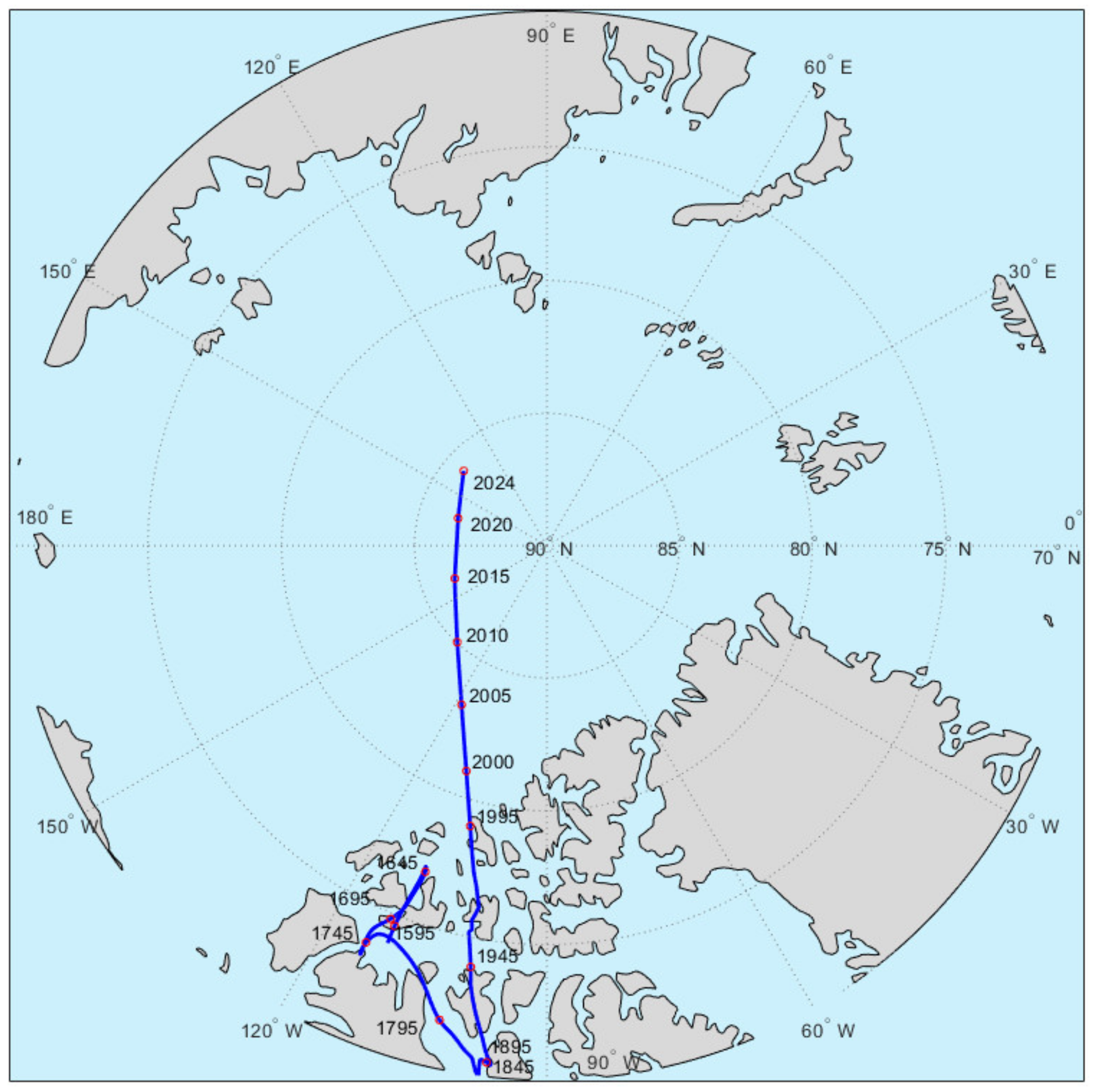
(a) The Magnetic North Pole was in Northern Canada 30 years ago. Now, the Magnetic North Pole has just left Canada, travelling at a growing speed, from 15 km/year until 2005, up to 60 km/year now, heading probably to Siberia (
Figure 10). An excellent article [
13], explains this phenomenon to the limits of our current knowledge and offers this itinerary of the Magnetic North Pole over the past two centuries. Siberia is no new place for the Magnetic North Pole; last time it was probably there was in 1300 BC. “… Over the last 7000 years, [the North Magnetic Pole] seems to have chaotically moved around the geographic pole, showing no preferred location” [
13]. The Magnetic South Pole is in Antarctica and also wanders, but it does it independently from its North counterpart. The significant fact is that the wander speed quadrupled in the past decades, breaking all records since the collection of these measurements was started.
(b) The magnetic field of the Earth has weakened by 20% over the last two centuries and its evolution cannot be predicted.
Not only reversals completely wreck the navigation based on Magnetic North but also tentative reversals. The amplitude of their movement is, however, just as disturbing for navigation as the reversal itself.
Using the chronology data from [
8], in the past 50 mil years, we may estimate the probability of the next major event (Chron, Subchron) in the following 100 years. Normal polarity intervals add up to approximately 13.74 mil years, and the number of events (Chrons, Subchrons) is 77. Therefore, the probability of an event in the next year is
The probability it does not happen in 100 years is
Consequently, the probability of a reversal happening in the next 100 years is
This basic statistic calculation assumes (i) that the phenomenon is purely random, which it obviously is not; in addition, (ii) the calculation does not take into account the fact that a new reversal is long overdue, and (iii) that our present-day polarity is less likely than the reversed polarity. Also, (iv) the precursor symptoms are not considered, but this is just based on common sense; there is no scientific proof that these are indeed precursor symptoms. The methods of scientific research into the past of the Earth do not identify precursor symptoms. Assumption (i) is expected to overestimate the result, whereas Approximations (ii), (iii) and (iv) are expected to underestimate the result. A geomagnetic expert evaluation of this probability would be a major advance in this research. This paper is just suggesting a very approximate, probably underestimated value. The time horizon of 100 years was chosen as being the approximation of the history of aviation up to this point, when such a major change is considered.
From the air navigation perspective, the above uncertainty over the pole reversals and tentative reversals is disturbing. Recent published research found the above-mentioned probable duration of a reversal of the order of 100 years [
10]. This aggravates the impact on navigation, since it indicates a high rate of change, of 1.8° of VAR per year on average. Assuming the probability distribution, this could lead to some airports being impacted by a change of 3° per year. Currently, aeronautical charts aligned to MN use an Annual Rate of Change (ARC) in VAR, which is expressed in minutes of arc annually. This method is practical to update VAR on assumptions of linearity and predictability, justified because the correction is small. However, at 1.8° annually on average, its non-linear and unpredictable nature makes it impractical for maintaining the aeronautical chart database.
Even if the probability of a pole reversal or tentative pole reversal is small, aviation needs to consider a contingency plan for this situation, as indeed it does for all other improbable situations. In case MN is replaced by TN, the threat is no longer effective, and this is the case with maritime navigation. Essentially, the contingency plan for such an event would be the transition to TN.
In essence, the magnetic field of the Earth is changing, irregular, and unpredictable, and sensing it on board an aircraft is challenging. It is hardly a good choice of reference, if it were a choice. In over a century, the aviation community has become accustomed to it as the forced choice of reference for horizontal navigation. In the next chapter, the consequences for aviation of these variabilities are analysed.
4. Consequences of an Unstable and Irregular Directional Reference on Aviation
Using MN as a reference presents the following factors of uncertainty, which add to the magnetic compass inherent errors, to create a glum picture of using MN as a reference for aviation:
VAR is an irregular function in space and time: VAR (LAT, LONG, date);
ARC is the annual rate of change in VAR in a certain place: ARC (LAT, LONG, date);
The ARC model assumes a linear change in VAR, but the real phenomenon is non-linear (so the ARC itself needs to be corrected);
Navigation databases need to maintain the VAR and ARC variables;
Magnetic thunderstorms cause significant deviations from the expected VAR;
A magnetic pole reversal or reversal tentative could start anytime, with a small probability (not zero, though), and in this case the current system managing VAR/ARC could fail.
(i) Due to its irregular nature (illustrated in
Figure 5), the magnetic directional reference does not support navigation equations, navigation optimisations or mathematical modelling. In order to use any mathematical support, one has to convert all azimuths to True North, apply the methods, and then the results back to Magnetic North. Magnetic North reference is an irregular local function and therefore is not consistent for solving navigation equations. All mathematical models for navigation and for optimised trajectories require a True North reference frame. This means that all the magnetic azimuths need to be converted to true azimuths using the VAR correction; then, the results need to be converted back to magnetic.
(ii) Aeronautical charts require to be rotated from time to time to cope with the VAR changes, since they are aligned to MN.
(iii) Aeronautical information databases (ARINC-424) require periodical updates and costly maintenance operations due to the VAR changes over the years, since all flight trajectories and flight procedures are aligned to MN.
(iv) Omnidirectional radio navigation aids (VOR, TACAN) require recalibration from time to time, and present a residual calibration error in between these changes.
(v) The magnetic field of the Earth has a horizontal component which is maximum at the magnetic equator but decreases to the magnetic poles (following a cosine of magnetic latitude law), making its measurement impractical in the polar regions; ICAO limits the use of MN reference to between 75° N and 63° S of latitude.
(vi) Runway identifiers are based on their magnetic heading, rounded to the nearest 10 degrees. Due to the changes in local VAR over the years, sometimes the magnetic azimuth of a runway demands the change in the runway identifiers, which is a costly operation (as presented further), with multiple implications for the navigation charts and databases, and redrawing of the runway markings.
(vii) Wind directions are provided by the meteorological systems in a TN reference. In order to be used for runway operations (take-offs and landings), surface wind direction has to be converted to MN using the local VAR by the air navigation service providers (ANSP). Aloft winds are still given in the TN reference. There is a lack of operational uniformity in this respect.
The requirements of aeronautical information changes mentioned in (ii), (iii), (iv) and (vii) apply when the VAR accumulates total changes of 1°, with the exception of (vi), which apply when accumulating total changes of 10°. The period between these changes results from the location in the chart in
Figure 11.
In the polar regions, the MN reference is waived de jure; for example, air navigation in Northern Canada is already based on TN [
1,
14]. Also, during magnetic thunderstorms, the MN reference is waived de facto.
The segment of air navigation which is the most vulnerable to magnetic field changes is the flight in the terminal phases: departures and approaches and TMA navigation. The reason for this is the fact that runway directions need to be updated when the MN changes over the years by more than 1°. All tracks in the aeronautical charts use the MN reference and need to be updated. Most IFR aeronautical charts serve the terminal phases (instrument approach and departures, SIDs, STARs). All navigation databases (ARINC-424) need updates.
Even more disturbing are the accumulated annual changes for the identification of runways. These need updates when the magnetic variation changes exceed 10°, because runways are named, in principle, in tens of degrees track from MN. For example, Zurich Airport will relabel all three runways from May 2024 (six runway directions). Such an RWY designator change operation requires preparations for years in advance and costs approximately EUR 3 mil for three runways, according to the Airport of Zurich data [
15]. The breakdown of the costs is as follows: EUR 2 mil for the airport side (markings of runways) and EUR 1 mil for the ANSP side. Other examples are found in the USA: [
16] reveals that the two directions of the runway at John Wayne airport cost USD 885 k (81% paid with FAA grants) to redesignate. In [
17], the cost of USD 800 k per runway (both directions) is quoted at Wichita, KA. In [
18], it is revealed that Fairbanks International Airport in Alaska redesignated runway 1L-19R to 2L-20R in 2009 when the MN shifted enough to mandate a change at a cost of UED 1,244,000. And the airport operators know—from NCEI’s World Magnetic Model [
4] and other sources—that they will likely need to update the identifier again in 2033. In the subsequent calculations, we would assume an average cost of USD 1 M per runway redesignating operation.
As a consequence of the annual variability in time of the magnetic field of the Earth, in
Figure 7, all international airports are represented on a world map with isogradient curves in minutes of arc per year of MN change (ARC). In this representation, the absolute value of ARC is relevant, not that of the signed ARC, because the objective is to calculate the mean time in years between 1° shifts and 10° shifts, respectively. The sign of ARC does not make any difference.
Table 3 represents the equivalence between ARC and the mean time between the shifts based on these simple equations:
The Zurich Airport case confirms
Figure 11, because the redesignating of the runways in 2024 follows the previous one in 1948, i.e., 76 years. MTBC1 for Zurich is found between the six and eight isochrones; thus, the MTBC10 is between 60 and 80 years [
13].
Using the AIRAC international airport database with the number of runways in 2023 [
3] and the geomagnetic data provided in [
4], the following results are obtained from the data analysis.
In total, AIRAC publishes 13,833 airports worldwide with 35,089/2 runways. Each runway has two directions in principle, but there are exceptions. The following airports publish just one direction for one of their runways: EDDF, EDDW, EGLC, EGPD, HUEN, LFMF, NZWD, SBMQ, SCCI, SCIP, ZUTF. Using a Matlab application, the authors calculated the number of runways affected by a shift of 1° in VAR each year: 1763 runways worldwide. Similarly, 176.3 runways require redesignating operations each year due to the accumulation of a 10° change in VAR.
The breakdown of the result on airports with a certain number of runways is given in
Table 4. It could serve to further research for assessing a more realistic impact of redesignating the runways.
The prototype of this analysis was put forward in [
1,
19]. The one below was conducted independently, though, with the intention to verify the validity of the results.
Using an approximate cost of USD 1 mil. for redesignating one runway at MTBC
10 and the conservative approximate cost of USD 0.1 mil. for updating aeronautical charts, databases, and flight procedures at MTBC
1, the rough estimate of the total worldwide annual cost of using MN as a reference was calculated:
Even though there are airports where the RWY redesignating schedule is delayed as cost cut measures, the total costs are not influenced by this delay. In the long run, all the changes are finally performed.
This is only the cost of the airports and air navigation service providers. Additional costs arise from using MN for flight operators, for aircraft and avionics manufacturers. In [
20], the average FMS/IRU MAGVAR update costs are estimated at USD 4 k per year per commercial aircraft. The worldwide fleet of 25,000 commercial aircraft currently in service [
21] would require update costs of approximately USD 100 mil annually.
Transition to TN (which is a stable and regular reference) would eliminate all these problems and their associated costs.
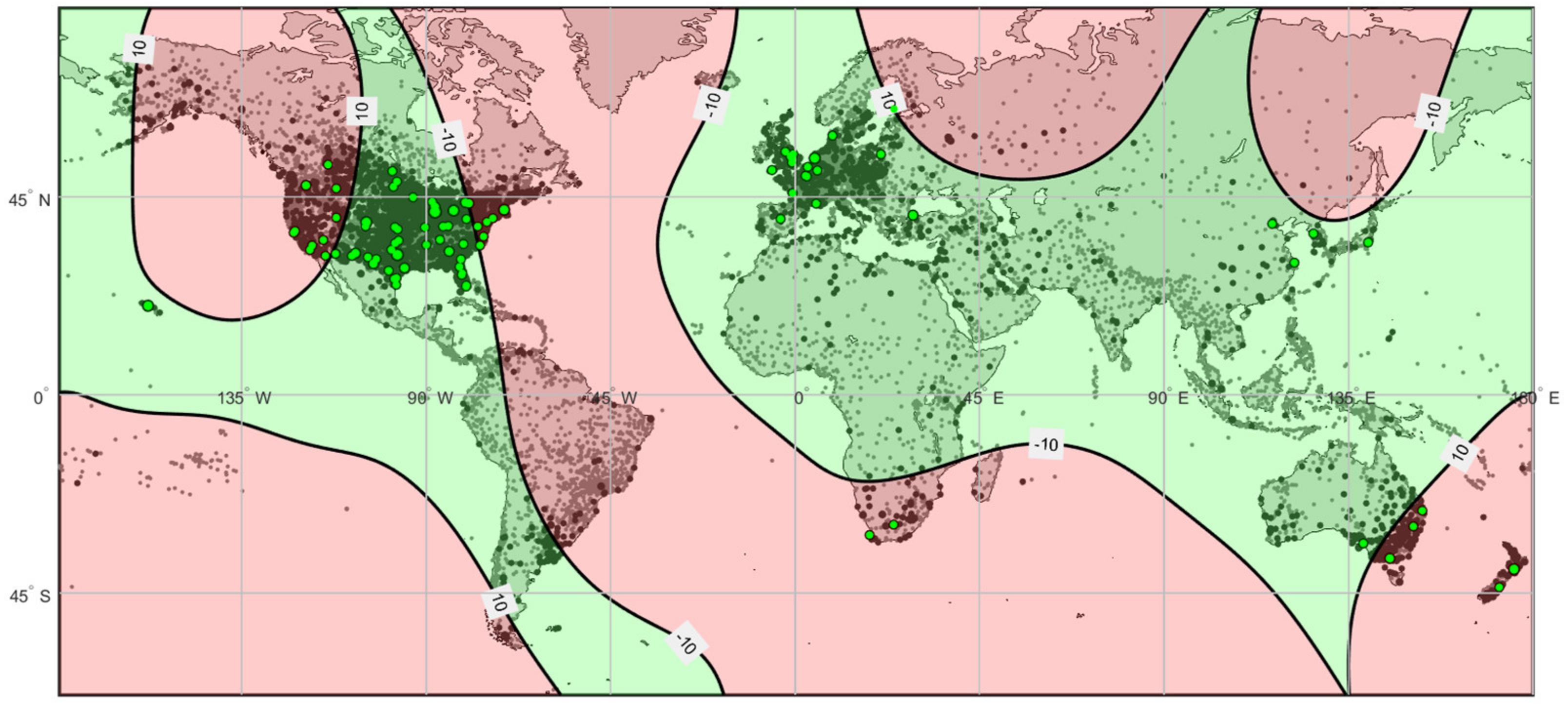
One of the main arguments against the adoption of the TN is the massive cost of redesignating all the runways in the world according to the new azimuth reference. In this paper, we analysed the estimate of this cost and contrasted it to the benefits of the adoption of TN. Out of the total 17,544.5 runways worldwide in the AIRAC database [
3], 12,139.5 runways do not need redesignating at all, since they are already within a ±10 range of the VAR. In principle,
Figure 12 shows the regions where these airports are found with a greater probability, but the number above was calculated individually per each runway, with the current VAR of each runway.
The rest of 5405 runways would require redesignating, and we assume that it would take 10 years for this transition. The NPV analysis in
Table 4 uses time intervals of 10 years and calculates the NPV of both variants: preserve MN and transition to TN for the next 40 years. The classic NPV equation is used (
C0 = 0):
Table 5 considers the yearly costs of maintaining MN previously calculated of USD 352.6 M plus the USD 100 M, which mean USD 4526 M per 10 years. This is contrasted to the TN transition variant, which would require USD 5405 M up front in the first 10 years. The opportunity cost of capital
r was considered 5% p.a. (74% aggregated per 10 years), but the results are not sensitive to the choice of
r. The NPV of the TN switching scenario is much better than the MN preserving scenario, and the conclusion is not sensitive to the choice of
r.


