LCF Lifetime Reliability Prediction of Turbine Blisks Using Marine Predators Algorithm-Based Kriging Method

Abstract

To achieve the low-cycle fatigue (LCF) lifetime prediction and reliability estimation of turbine blisks, a Marine Predators Algorithm (MPA)-based Kriging (MPA-Kriging) method is developed by introducing the MPA into the Kriging model. To obtain the optimum hyperparameters of the Kriging surrogate model, the developed MPA-Kriging method replaces the gradient descent method with MPA and improves the modeling accuracy of Kriging modeling and simulation precision in reliability analysis. With respect to the MPA-Kriging model, the Kriging model is structured by matching the relation between the LCF lifetime and the relevant parameters to implement the reliability-based LCF lifetime prediction of an aeroengine high-pressure turbine blisk by considering the effect of fluid–thermal–structural interaction. According to the forecast, when the allowable value of LCF lifetime is 2957 cycles, allowing for engineering experience, the turbine degree of reliability is 0.9979. Through the comparison of methods, the proposed MPA-Kriging method is demonstrated to have high precision and efficiency in modeling and simulation for LCF lifetime reliability prediction of turbine blisks, which, in addition to the turbine blisk, provides a promising method for reliability evaluation of complicated structures. The work done in this study aims to expand and refine mechanical reliability theory.

1. Introduction

As critical components of an aviation engine, high-pressure turbine blisks operate under severe environments of high temperature, corrosion, and strong centrifugal force. As a result, fatigue failures are common problems for actual turbine blade applications in the field [1,2]. Herein, the low-cycle fatigue (LCF) of the turbine blisk is a common failure mode and directly affects the safety and reliability of aeroengine operation, which is recently the main research focus [3,4]. Therefore, it is essential to exhaustively analyze the reliability-based LCF lifetime forecast of turbine blisks for optimum performance.

In the field of structural reliability estimation, numerous analytical approaches have been proposed, which include direct and indirect methods (also called surrogate model methods). The direct methods mainly involve Monte Carlo (MC) [5], first-order second-moment (FOSM) [6], advanced first-order second-moment (AFOSM) [7], and so on. The MC method requires thousands of simulations to reliably achieve the study objective, which has the weakness of being very time-consuming for the probabilistic analysis of structural finite elements. The approximate analytical method (e.g., the FOSM and AFOSM) is suitable for structural reliability analysis with known performance function. These traditional methods have been widely used and have proven to be practicable and productive in a variety of fields [8,9,10,11]. However, the reliability-based LCF lifetime prediction of the high-pressure turbine blisk involves multi-discipline (heat, dynamics, vibration), multi-failure modes (stress, strain, fatigue, and so on). For such complex causes, the traditional reliability approaches show limitations in computational accuracy and efficiency. Furthermore, to predict the non-linear models of the fatigue lifetime and damage and overcome the existing problems with the direct method in computational efficiency [12,13,14,15], the surrogate modeling methods like FOSM, FOR, SOR, SVM, ANN, and Kriging-based are then developed to accomplish structural reliability analysis and are commonly utilized to execute the reliability estimation of complicated structures’ LCF lifetime [16,17]. Although the surrogate modeling methods enhance the computational effectiveness of the LCF lifetime reliability evaluation, it is difficult to obtain an acceptable analytical precision in the LCF lifetime reliability estimation of complex structures. It is critical that effective surrogate approaches be developed with the goal of improving the LCF lifetime reliability estimation of complex structures in computational accuracy.

Wherein, Kriging is a powerful surrogate model which can provide a high-accuracy fitting function of the dependent variables and independent variables [18,19]. Lu et al. proposed the BIMEM method based on Kriging, LSM, and MLS methods that is established for the purpose of developing probability-based dynamic LCF estimation for turbine blisks [20]. Slot et al. used the PCE-based Kriging method to accomplish an LSF for measuring wind turbine fatigue reliability [21]. Huang et al. explored the AK-TCR-SM method based on the secant and Kriging model to solve the safety analysis issues [22]. These Kriging-based surrogate modeling methods can significantly reduce the computational cost compared to traditional surrogate models. However, the above-mentioned approaches, such as the least squares method (LSM), are incapable of accurately reflecting the extreme correlation between the dependent variables and independent variables. That is because the accuracy and efficiency of the method cannot meet the engineering requirement. Thus, it is significant to propose an applicable optimization algorithm for establishing a surrogate model.

The aim of this paper is to develop the Marine Predators Algorithm (MPA)-based Kriging (MPA-Kriging) method by introducing MPA for calculating the optimal parameters in Kriging, to improve the modeling and simulation accuracies of the Kriging model for exploring the reliability-based LCF lifetime prediction of the turbine blisk, with regard to fluid–thermal–structural interaction. In addition, the proposed MPA-Kriging method is validated by comparison with many methods. MPA is a new nature-inspired metaheuristic algorithm [23], used as an estimation technique for the Kriging model’s parameters to estimate these parameters accurately. Islam et al. applied MPA and probabilistic models to assess reliability accurately for open-source software [24]. Mohamed et al. proposed a novel enhanced MPA for parameter identification of static and dynamic PV models [25]. These works show the wide application of MPA.

The remainder of this paper is organized as follows: theory and methods, case study, methods validation, and conclusions. In Section 2, the basic theory of the MPA-Kriging method is investigated, involving the Kriging method, MPA, and the mathematical model of the MPA-Kriging method. Section 3 gives the implementation process for LCF lifetime reliability prediction using the proposed MPA-Kriging method. Section 4 conducts the LCF lifetime reliability prediction, comprising deterministic analysis, modeling, and reliability estimation. Section 5 validates the proposed methods by comparing them to methods such as the RSM and the traditional Kriging model, in terms of modeling ability and simulation capability. Finally, the conclusions of this study are summarized in Section 6.

2. Theory and Methods

2.1. Kriging Method

The revised Manson-Coffin model is often used for structural LCF lifetime prediction [26,27], i.e.,

$$\frac{\mathrm{\Delta }{\epsilon }_t}{2}=\frac{\mathrm{\Delta }{\epsilon }_e}{2}+\frac{\mathrm{\Delta }{\epsilon }_p}{2}=\frac{{\sigma }_f^{\prime }-{\sigma }_m}{E}{\left(2N_f\right)}^b+{\epsilon }_f^{\prime }{\left(2N_f\right)}^c$$

(1)

where $\mathrm{\Delta }{\epsilon }_t$ is the general values of strain amplitude; $\mathrm{\Delta }{\epsilon }_e$ denotes the elastic strain amplitude; $\mathrm{\Delta }{\epsilon }_p$ indicates the plastic strain amplitude; $E$ expresses the material elastic modulus; ${\sigma }_f^{\prime }$ and ${\epsilon }_f^{\prime }$ stand for the strength and ductility coefficients, respectively; ${\sigma }_m$ is the mean stress; $N_f$ is the turbine blisk LCF; $b$ and $c$ are the fatigue strength and ductility exponents.

From Equation (1), we can find that the LCF lifetime of turbine blisk is related to the strain amplitude, mean stress, strength coefficient, ductility coefficient, fatigue strength exponent, and fatigue ductility exponent.

The MPA-Kriging method is developed from the Kriging model and MPA, in which the MPA is employed to replace the gradient descent methods to search the optimal values of hyperparameters in the Kriging model. In this paper, the LCF lifetime prediction model of turbine blisk is established based on the Kriging model, and the relevant parameters of this model [13,28] are expressed by

$$\left\{\begin{array}{l}{N}_f\left(\mathit{x}\right)=f\left(\mathit{x}\right)=a_0+{\mathit{b}}_0\mathit{x}+{\mathit{x}}^T{\mathit{c}}_0\mathit{x}+z\left(\mathit{x}\right)\hfill \\ \mathit{x}={\left(\mathrm{\Delta }{\epsilon }_t,{\sigma }_m,{\sigma }_f^{\prime },{\epsilon }_f^{\prime },b,c\right)}^T\hfill \end{array}\right.$$

(2)

In Equation (2), the model consists of two components: linear and stochastic. The linear model can be written as a quadratic polynomial. Herein, $a_0$ is the constant term, ${\mathit{b}}_0$ is the vector of the linear term, and ${\mathit{c}}_0$ is the matrix of the quadratic term. And the symbols ${\mathit{b}}_0$ and ${\mathit{c}}_0$ can be described as

$$\left\{\begin{array}{l}{\mathit{b}}_0=\left(\begin{array}{cccccc}{b}_{0,1}& b_{0,2}& b_{0,3}& b_{0,4}& b_{0,5}& b_{0,6}\end{array}\right)\hfill \\ {\mathit{c}}_0=\left(\begin{array}{cccccc}{c}_{0,11}& c_{0,12}& c_{0,13}& c_{0,14}& c_{0,15}& c_{0,16}\\ c_{0,21}& c_{0,22}& c_{0,23}& c_{0,24}& c_{0,25}& c_{0,26}\\ c_{0,31}& c_{0,32}& c_{0,33}& c_{0,34}& c_{0,35}& c_{0,36}\\ c_{0,41}& c_{0,42}& c_{0,43}& c_{0,44}& c_{0,45}& c_{0,46}\\ c_{0,51}& c_{0,52}& c_{0,53}& c_{0,54}& c_{0,55}& c_{0,56}\\ c_{0,61}& c_{0,62}& c_{0,63}& c_{0,64}& c_{0,65}& c_{0,66}\end{array}\right)\hfill \end{array}\right.$$

(3)

Additionally, the stochastic model is a Gaussian random field, which satisfies

$$\left\{\begin{array}{l}Cov\left. [z\left({\mathit{x}}^i\right),z\left({\mathit{x}}^j\right)\right]={\sigma }^{2}R\left(\mathit{\theta },{\mathit{x}}^i,{\mathit{x}}^j\right)\\ R\left(\mathit{\theta },{\mathit{x}}^i,{\mathit{x}}^j\right)={\displaystyle \prod _{k=1}^6{R}_k\left({\theta }_k,x_k^i-x_k^j\right)}\\ E\left. [z\left(\mathit{x}\right)\right]=0\\ Var\left. [z\left(\mathit{x}\right)\right]={\sigma }^2\\ \mathit{\theta }=\left(\begin{array}{cccccc}{\theta }_1& {\theta }_2& {\theta }_3& {\theta }_4& {\theta }_5& {\theta }_6\end{array}\right)\end{array}\right.$$

(4)

in which k = 1, 2, …, 6 is the number of input parameters; i, j = 1, 2, …, m, m is the number of samples; ${\sigma }^2$ is the variance; $R\left(•\right)$ is the correlation function; $\mathit{\theta }$ is the vector of hyperparameter in the Kriging meta-model; $R_k\left({\theta }_k,x_k^i-x_k^j\right)$ is the kth kernel function of the correlation function.

Then, Gaussian kernel is employed in this case because of its high processing capability [29]. The correlation function is

$$R\left(\mathit{\theta },{\mathit{x}}^i,{\mathit{x}}^j\right)=\exp \left(-{\displaystyle \sum _{k=1}^6{\theta }_k{\left(x_k^i-x_k^j\right)}^2}\right)$$

(5)

The gradient descent method (GDM) is employed to resolve the hyperparameters, i.e.,

$$\underset{\mathit{\theta }}{\max } L\left(\mathit{\theta }\right)=-\left(m\ln \left({\widehat{\sigma }}^2\right)+\ln \left|\mathit{R}\right|\right)$$

(6)

where ${\widehat{\sigma }}^2$ is the prediction variance.

2.2. Marine Predators Algorithm

In the traditional Kriging method, the GDM is unable to ensure to be a Globally Optimal Solution (GOS) for high-nonlinear problems. To address this issue, the MPA is applied to settle the minimizing optimization into which the maximizing optimization of high-nonlinear solution is transformed, i.e.,

$$\begin{array}{l}\underset{\mathit{\theta }}{\min } \phi \left(\mathit{\theta }\right)={\left|\mathit{R}\right|}^{\frac{1}{m}}{\widehat{\sigma }}^2\\ \mathrm{s}.\mathrm{t}. {\theta }_k>0\end{array}$$

(7)

With respect to Ref. [30], the detailed processes of searching the optimal hyperparameters with the MPA are summarized in Figure 1. The optimization process of using MPA to search for the hyperparameters of the Kriging model is described as follows:

Step 1: Set relevant parameters and initialize the population;

Step 2: Calculate the fitness value, and record the optimal position;

Step 3: Predators select the corresponding update method to update the predator position according to the iteration stage;

Step 4: Compute the fitness value and update the optimal position,

Step 5: Jump to Step 3 to update the fitness and predator position when the results do not meet the requirement of precision or the stop conditions. Otherwise, jump to Step 6.

Step 6: Output the optimal hyperparameters when the analytical results satisfy the stop conditions.

2.3. Marine Predators Algorithm-Based Kriging Method

In line with the obtained hyperparameters, the LSM is used to resolve the unknown matrix $\mathit{d}$, i.e.,

$$\mathit{d}={\left({\mathit{F}}^T{\mathit{R}}^{-1}\mathit{F}\right)}^{-1}{\mathit{F}}^T{\mathit{R}}^{-1}\mathit{Z}$$

(8)

in which $\mathit{d}=(a_0,b_0,c_0)$; both $\mathit{F}$ and $\mathit{Z}$ are the matrix of basis functions and the vector of outputs, respectively, with respect to $m$ samples with the samples.

In addition, the stochastic model at a point ${\mathit{x}}_{*}$ is represented as

$$z\left({\mathit{x}}_{*}\right)={\mathit{r}}_z^T\left({\mathit{x}}_{*}\right){\mathit{R}}^{-1}\left(\mathit{Z}-\mathit{F}\mathit{d}\right)$$

(9)

Here, ${\mathit{r}}_z\left({\mathit{x}}_{*}\right)$ is the correlation matrix of ${\mathit{x}}_{*}$ and $\mathit{x}$. And ${\mathit{r}}_z\left({\mathit{x}}_{*}\right)$ is described as

$${\mathit{r}}_z\left({\mathit{x}}_{*}\right)=\left(\begin{array}{cccc}R\left(\mathit{\theta },{\mathit{x}}_{*},{\mathit{x}}^1\right)& R\left(\mathit{\theta },{\mathit{x}}_{*},{\mathit{x}}^2\right)& \cdots & R\left(\mathit{\theta },{\mathit{x}}_{*},{\mathit{x}}^m\right)\end{array}\right)$$

(10)

Through the above analysis, the MPA-Kriging model is derived, and then it will be applied to accomplish the LCF prediction of turbine blisks.

3. LCF Lifetime Reliability Estimation Methods for Turbine Blisks

3.1. Reliability Estimation Principles

In the MPA-Kriging model, the turbine blisk reliability estimation LSF is

$$g\left(\mathit{x}\right)=N_f\left(\mathit{x}\right)-N_{f,allow}$$

(11)

where $N_{f,allow}$ is the maximum allowable lifetime. If $g\left(\mathit{x}\right)\ge 0$, the turbine blisk structure is safety; otherwise, $g\left(\mathit{x}\right)<0$ illustrates that the structure is failure.

In this paper, the MC sampling method [31] is used for determining the turbine blisk lifetime degree of reliability by LSF. Additionally, the degree of reliability $p_r$ is

$$\left\{\begin{array}{l}\begin{array}{cc}{p}_r& ={\displaystyle {\int }_{r}g\left(\mathit{x}\right)d\mathit{x}}={\displaystyle \int I_r\left(g\left(\mathit{x}\right)\right)g\left(\mathit{x}\right)d\mathit{x}}\hfill \\ & =E\left. [I_r\left(g\left(\mathit{x}\right)\right)\right]=\frac{1}{N}{\displaystyle \sum I_r\left(g\left(\mathit{x}\right)\right)}=\frac{N_r}{N}\hfill \end{array}\hfill \\ s.t. I_r\left(g\left(\mathit{x}\right)\right)=\left\{\begin{array}{l}0, g\left(\mathit{x}\right)<0\\ 1, g\left(\mathit{x}\right)\ge 0\end{array}\right.\hfill \end{array}\right.$$

(12)

in which $r$ is the margin of safety; $I_r\left(•\right)$ is the indicator function for the margin of safety; $N_r$ is the number of samples located in the margin of safety; $N$ is the general number of samples.

3.2. The Flowchart for LCF Lifetime Reliability Estimation with the MPA-Kriging Method

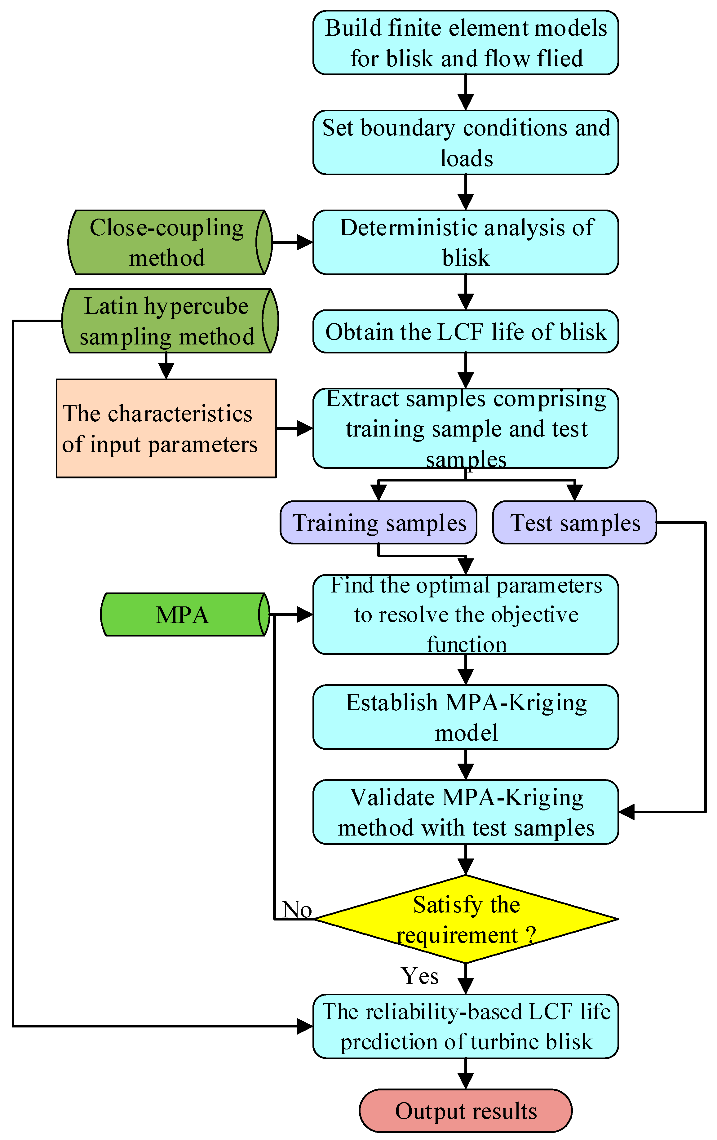
To establish the MPA-Kriging-based LCF lifetime prediction model, we obtained the optimal two-part parameters of Kriging and conducted the turbine blisk LCF lifetime reliability analysis based on the prediction model. The flowchart for turbine blisk LCF lifetime prediction and reliability analysis using the MPA-Kriging method is shown in Figure 2. The detailed procedures for the reliability-based LCF lifetime prediction of turbine blisks using the MPA-Kriging method are described as follows:

Step 1: Establish the three-dimensional (3D) model of turbine blisk and operating ambience.

Step 2: Generate their finite element (FE) models.

Step 3: Set boundary conditions and loading parameters.

Step 4: Derive deterministic analysis of turbine blisk using the close-coupling method, and the blisk lifetime is obtained by simulation calculation.

Step 5: Determine the numerical features of the input parameters to extract their samples using the LHS method [32,33] and obtain their LCF lifetime.

Step 6: Divide the samples into training and test sequences.

Step7: Based on the MPA method, the hyperparameters of the Kriging model are found through the training sequences.

Step 8: Adopt the optimal hyperparameters to obtain the values of unknown coefficients and develop the MPA-Kriging model.

Step 9: Validate the advantages of the MPA-Kriging model through the testing sequences, from modeling efficiency and precision. If this model satisfies the requirements, jump to Step 10; conversely, return to Step 7.

Step 10: Conduct the reliability analysis of the LCF lifetime using the established MPA-Kriging model and the MC method.

4. The LCF Lifetime Reliability Estimation of Turbine Blisks

4.1. Deterministic Analysis of Turbine Blisk LCF Lifetime

A turbine blisk is a cyclically symmetric structure that is subject to complicated loads from multiple physical sources. To simulate the LCF lifetime, we built a 3D model of a 1/48 turbine blisk and flow field covering three blades as the study objects. The blisk and flow field were established with tetrahedron elements as shown in Figure 3.

We constructed five meshes with various element sizes to look into the convergence analysis of the FE model. The purpose was to acquire the credibility finite element model for dynamic deterministic analysis.

Table 1. Validation of FE model with different element sizes.

Cell Sizes, m	Number of Cells		Maximum Values of Intermediate Outputs
	Blisk	Flow Field	Stress, ×108 Pa	Strain, ×10−3 m/m
0.03	2725	189	9.3825	5.1325
0.02	8066	1428	9.5614	5.3253
0.01	59,877	8826	9.7034	5.4762
0.008	115,429	16,299	9.8716	5.5376
0.005	467,470	37,863	9.8717	5.5378

and Figure 4 display the analytical findings.

From Table 1 and Figure 4, it is denoted that the turbine blisk simulation results converge to a constant ($\mathrm{Stress}\approx 9.8717\times {10}^8\mathrm{Pa}$, $\mathrm{Strain}\approx 5.5378\times {10}^{-3}\mathrm{m}/\mathrm{m}$) with the decrease in the number of elements, and the turbine blisk LCF lifetime converges to a constant of 4719 with the increase in the number of elements.

By weighting the computation complexity, the dynamic deterministic analysis of the turbine blisk is carried out using a unit size of 0.008 m and a total number of units of 131,725. This is because the analytic error of turbine blisk LCF lifetime is 011% in comparison with the finest element size.

To obtain turbine blisk LCF lifetime, the time domain [0 s, 215 s] is regarded in this study, which includes 12 critical points [34]. GH4133 is considered to be the material of the turbine blisk, and the density, elastic modulus, and Poisson’s ratio of the material are 8560 kg/m³, 1.61 × 10¹¹ Pa, and 0.3224, respectively. Inlet velocity and inlet pressure are assumed to be 124 m/s and 588,000 Pa, respectively. Additionally, the gas temperature and rotational velocity are time-dependent variables, as shown in

Table 2. The change in gas temperature and rotational velocity in time domain [0, 215 s].

Time, s	0	10	95	100	130	140	150	160	165	200	205	215
Gas temperature, K	50	468	573	782	697	838	924	1052	1200	1200	998	998
Rotate speed, m/s	0	420	448	656	748	852	654	1054	1168	1168	950	950

.

In light of the material parameters and loads, the transient deterministic analysis of the turbine blisk was adopted by the coupling technique and finite volume method considering the effect of fluid, thermal, and structural loads. The multi-physical coupling analysis technique was developed in [35,36,37]. The simulation result (stress and strain) distributions during the time domain [0 s, 215 s] are acquired in Figure 5.

As the gas temperature and rotation speed increase, the stress and strain on the turbine blisk increase, and their maximums are in the rising stage in [165 s, 200 s] in Figure 5. Therefore, t = 175 s is regarded as the time point to probe into the turbine blisk stress, strain, and LCF lifetime distributions, the nephograms of which are displayed in Figure 6. In Figure 6, $\sigma$ and $\epsilon$ are the turbine blisk’s stress and strain. Additionally, the root of blade takes on the maximum of turbine blisk stress and strain in Figure 6.

4.2. Turbine Blisk LCF Lifetime Modeling

Actually, during the design and operation of aeroengine blisk, the above influence factors indeed have much randomness. This is the reason that probabilistic analysis is necessary for the LCF lifetime analysis of turbine blisks in terms of the randomness of these parameters involving material performance parameters and load parameters. According to engineering experience, it is deduced that the input variates are random. These variables for turbine blisk LCF lifetime comprised the inlet velocity $\mathit{v}$, outlet pressure ${\mathit{p}}_{\mathit{o}\mathit{u}\mathit{t}}$, gas temperature ${\mathit{t}}_{\mathit{g}}$, material density $\rho$ and rotational velocity $\omega$, strength coefficient ${\sigma }_f^{\prime }$, ductility coefficient ${\epsilon }_f^{\prime }$, fatigue strength exponent $\mathit{b}$, and fatigue ductility exponent $\mathit{c}$. As shown in

Table 3. Numerical attributes and distributional properties of input parameters.

Variables	Mean	Std. Dev.	Distribution
Inlet Velocity v, m/s	124	16	Normal
Outlet Pressure pout, Pa	588,000	58,800	Normal
Gas Temperature tg, K	1200	120	Normal
Density ρ, kg/m3	8560	428	Normal
Rotational Velocity w, rad/s	1168	68	Normal
$\mathbf{Strength}\mathbf{coefficient}{\sigma }_f^{\prime }$, ×106 Pa	1318	68	Normal
$\mathbf{Ductility}\mathbf{coefficient}{\epsilon }_f^{\prime }$	0.976	0.096	Lognormal
Fatigue strength exponent b	−0.084	0.006	Normal
Fatigue ductility exponent c	−0.94	0.08	Normal

, which lists the numerical attributes and distributional properties, total input variables are assumed to be independent of each other.

In line with the numerical features and distribution features in Table 3, the Latin Hypercube Sampling method is adopted to extract a pool of 150 input samples. Turbine blisk LCF lifetime is obtained via deterministic analysis. We randomly selected 100 samples as the training samples to derive the mathematical model of turbine blisk LCF lifetime using the MPA-Kriging method, and the remaining sequences are treated as the testing sequences to validate the accuracy of the proposed MPA-Kriging model.

Combined with the theory shown in Section 2.2, we can build the MPA-Kriging model of turbine blisk LCF lifetime with the 50 training samples, which is as follows:

$$\left\{\begin{array}{l}{a}_0=-0.4380\\ b_0=\left(\begin{array}{cccccc}0.6833& 0.5731& 0.9298& 0.1369& -0.2149& -0.4119\end{array}\right)\\ c_0=\left(\begin{array}{cccccc}0.1583& 0.0623& 0.1912& 0.0258& -0.0623& -0.0615\\ 0.0623& 0.1333& 0.0485& 0.0440& -0.0153& -0.0094\\ 0.1912& 0.0485& 0.2117& 0.0130& -0.0767& -0.0652\\ 0.0258& 0.0440& 0.0130& -0.1305& -0.0051& 0.0088\\ -0.0623& -0.0153& -0.0767& -0.0051& 0.1209& -0.0963\\ -0.0615& -0.0094& -0.0652& 0.0088& -0.0963& 0.2462\end{array}\right)\\ r={\left(\begin{array}{cccc}0.0439& 0.0785& \cdots & -0.1105\end{array}\right)}_{1\times 100}\end{array}\right.$$

(13)

4.3. Reliability Estimation of Turbine blisk LCF Lifetime

The MC method is used to run 10,000 simulations in accordance with the LSF to accomplish the dependability calculation of the turbine blisk’s LCF lifetime. The analysis results are displayed in Figure 7.

Based on the distribution rules of input parameters, we input a set and randomized them to the established MPA-Kriging model, and then we could obtain one sample of turbine blisk LCF lifetime. Therefore, using the MC method, 10,000 sets of randomized parameters were transmitted to the model, and the LCF lifetimes of turbine blisk were recorded in Figure 7a. To obtain the rule of the 10,000 sampling LCF lifetimes, we count the times of each lifetime in Figure 7a and describe the distribution histogram of the data in Figure 7b, which is used for obtaining the distribution characteristics of the lifetime.

From Figure 7, the turbine blisk LCF life follows a lognormal distribution with a mean value of 1.7764 × 10⁴ cycles and a standard deviation of 4.932 × 10³ cycles, and the turbine blisk LCF lifetime’s degree of reliability is 0.9979 computed by Equation (7), as the allowable lifetime is 2957.

We adopted five different samples to validate the chosen reliability allowable lifetime based on the MC method. The evaluation results are shown in

Table 4. The turbine blisk LCF lifetime’s degree of reliability for different MC samples.

MC Samples	Degree of Reliability	Precision, %
102	0.960	3.86
103	0.983	1.751
104	0.9987	0.01
105	0.9986	—

, and the turbine blisk LCF lifetime’s degree of reliability under 10⁵ samples is regarded as the precision calculation standard.

Table 4 shows that the degree of reliability converges to 0.9986 as the number of samples increases. Compared with 10⁵ samples, the degree of reliability with 10⁴ samples is closest to 0.9987, which has a precision of 0.01%. Therefore, 0.9987 is selected as the precision calculation standard (10⁴ samples) for evaluating the turbine blisk.

5. Validation of MPA-Kriging Performance

5.1. Modeling Performance

To demonstrate the advantages of the MPA-Kriging method in modeling ability, the time consumption of modeling and prediction accuracy were validated with 50 testing samples by comparison of the RSM and Kriging models. The predictive precision was assessed by root mean squared error (denoted by RMSE), and the real LCF lifetimes of turbine blisk using the direct simulation method were treated as the standard. Additionally, the efficiency and accuracy improvement of the Kriging and MPA-Kriging methods are discussed based on the analysis results of the RSM method. The results are shown in

Table 5. Modeling ability of RSM, Kriging, and MPA-Kriging methods.

Methods	Modeling Time, s	Improved Efficiency, %	RMSE	Improved Precision, %
RSM	1.67	—	412.4581	—
Kriging	1.46	12.57	268.1544	34.98
MPA-Kriging	0.79	52.69	102.4512	75.16

.

As demonstrated in the second and third columns in Table 5, the modeling time consumptions for the proposed MPA-Kriging method (0.79 s) is about half those for the RSM and Kriging methods (1.67 s and 1.46 s). Moreover, compared with the RSM and Kriging methods, the modeling time of the MPA-Kriging method is less by 52.69% and 40.12%.

As shown in the last two columns of Table 5, the RMSE of the proposed MPA-Kriging method (102.4512 cycles) is less than for the RSM and Kriging methods (412.4581 cycles and 268.1544 cycles), and the precision of this MPA-Kriging method is enhanced by 75.16% and 40.18% with regard to the RSM and MPA-Kriging methods. Therefore, the proposed MPA-Kriging method has been presented to have better modeling accuracy and efficiency than the traditional gradient descent method since (1) the Kriging method can learn efficient data from training sequences and build the relationship between the dependent and independent variables, and (2) the MPA method can obtain the optimal variable values.

According to the analytical results, the developed MPA-Kriging approach shows distinct advantages in modeling speed and accuracy.

5.2. Simulation Capability

To elaborate the feasibility of the MPA-Kriging method for simulation capability, the direct simulation, RSM, and Kriging models were applied to accomplish the reliability estimation of turbine blisk LCF lifetime under 10², 10³, and 10⁴ simulations. In addition, the results of direct simulation are regarded as the standard for researching the simulation accuracy and efficiency. The results of simulation efficiency and precision are listed in

Table 6. Simulation efficiency of reliability estimation of turbine blisk LCF lifetime for four methods.

Method	Number of Simulations
	102	103	104
Direct simulation	56,845 s	624,464 s	—
RSM	1.02 s	1.74 s	4.36 s
Kriging	0.44 s	0.75 s	2.18 s
MPA-Kriging method

and

Table 7. Simulation precision of reliability estimation for four different methods.

Simulation	Degree of Reliability				Simulation Precision, %
	Direct Simulation	RSM	Kriging	MPA-Kriging Method	RSM	Kriging	MPA-Kriging Method
102	0.99	0.82	0.90	0.94	88.89	90.91	94.95
103	0.997	0.894	0.927	0.986	89.67	92.98	98.89
104	—	0.9398	0.9658	0.9979	—	—	—

.

From Table 6, it is demonstrated that the consumption time for modeling with different methods, namely the RSM, Kriging meta-model, and MPA-Kriging methods, is far less than that for direct simulation. The MPA-Kriging method is better than the RSM method in simulation efficiency. This can be explained by (1) surrogate models (they include RSM, Kriging, and MPA-Kriging), which are far smaller and outperform direct simulations (MC), (2) simulation time consumption of surrogate models is much less than for direct simulation as the number of simulation samples increases, and (3) the MPA-Kriging method is the minimal time consumption method among the three modeling methods due to introducing the MPA.

As shown in Table 7, the MPA-Kriging method holds the highest precision (96.92%) compared with the RSM and Kriging methods (89.28% and 91.95%). Additionally, due to the advantages with introducing the MPA, the MPA-Kriging method results in optimal parameter values with limited samples, which is almost equal to the direct simulation degree of reliability.

Therefore, the proposed MPA-Kriging method has apparent advantages in accuracy and efficiency.

6. Conclusions

This paper proposed a novel LCF lifetime prediction and reliability analysis MPA-Kriging method for turbine blisks based on the MPA and Kriging models. In this method, the gradient descent optimization method is replaced by MPA, which solves the hyperparameters of the Kriging model and is more accurate and efficient. In addition, we adopted the Latin Hypercube Sampling method to obtain 150 sets of input parameters in the LCF lifetime deterministic analysis of the turbine blisk based on FE simulation. Then, the reliability of the allowable LCF lifetime was calculated via the MC method. Ultimately, to verify the advantages of the MPA-Kriging method in terms of accuracy and efficiency capability, we compared it with three different conventional methods (direct simulation, RSM, and Kriging). Major conclusions are summarized as follows:

(1) To accomplish the dynamic deterministic analysis of the credibility finite element model, we chose the fittest element mesh size via the investigated convergence of the turbine blisk. The turbine blisk simulation results converge to a constant in which the LCF lifetime is 4719 cycles as the number of elements increases.

(2) To establish the fast and efficient MPA-Kriging surrogate model, the turbine blisk lifetimes were obtained by the FE and finite volume methods and by considering the effect of fluid, thermal, and structural loads. Therein, the turbine blisk analysis nephograms of FE simulation show that the root of blade takes on the maximum stress and strain, corresponding to the minimum lifetime.

(3) The hyperparameters of the Kriging model were calculated by considering it to be the optimization objective of MPA. The degree of reliability is 0.9979, computed by the MC method, while the allowable value of turbine blisk LCF lifetime is 2957, which can be used for structural strength reliability evaluation of the turbine blisk.

(4) Compared with other well-known models (direct simulation, RSM, and Kriging), the developed MPA-Kriging method outperformed all methods using different evaluation metrics. We can conclude that the developed MPA-Kriging method is an efficient Surrogate model that improves on the performance of the traditional Kriging model and enhances its prediction accuracy.

The efforts of this paper provide a promising way for the LCF lifetime reliability analysis of turbine blisks with high modeling precision and simulation efficiency, which have significance in mechanical reliability theory.

References

Wang, B.; Wang, C.; Shi, D.; Yang, X.; Li, Z. Assessment of Microstructure and Property of a Service Exposed Turbine Blade Made of K417 Superalloy. In IOP Conference Series: Materials Science and Engineering; IOP Publishing: Bristol, Britain, 2017; Volume 231, p. 012084. [Google Scholar]
Bjerager, P.; Krenk, S. Parametric sensitivity in first order reliability theory. J. Eng. Mech.1989, 115, 1577–1582. [Google Scholar] [CrossRef]
Der Kiureghian, A.; Lin, H.; Hwang, S. Second-Order Reliability Approximations. J. Eng. Mech.1987, 113, 1208–1225. [Google Scholar] [CrossRef]
Bucher, C.; Bourgund, U. A fast and efficient response surface approach for structural reliability problems. Struct. Saf.1990, 7, 57–66. [Google Scholar] [CrossRef]
Billinton, R.; Wang, P. Teaching distribution system reliability evaluation using Monte Carlo simulation. IEEE Trans. Power Syst.1999, 14, 397–403. [Google Scholar] [CrossRef]
Lu, C.; Fei, C.W.; Liu, H.T.; Li, H.; An, L.Q. Moving extremum surrogate modeling strategy for dynamic reliability estimation of turbine blisk with multi-physics fields. Aerosp. Sci. Technol.2020, 106, 106112. [Google Scholar] [CrossRef]
Kaymaz, I. Application of kriging method to structural reliability problems. Struct. Saf.2005, 27, 133–151. [Google Scholar] [CrossRef]
Acar, E. Reliability prediction through guided tail modeling using support vector machines. Proc. Inst. Mech. Eng. Part C—J. Mech. Eng. Sci.2013, 227, 2780–2794. [Google Scholar] [CrossRef]
Rajpal, P.S.; Shishodia, K.S.; Sekhon, G.S. An artificial neural network for modeling reliability, availability and maintainability of a repairable system. Reliab. Eng. Syst. Saf.2006, 91, 809–819. [Google Scholar] [CrossRef]
Gao, H.; Fei, C.; Bai, G.; Ding, L. Reliability-based low-cycle fatigue damage analysis for turbine blade with thermo-structural interaction. Aerosp. Sci. Technol.2016, 49, 289–300. [Google Scholar] [CrossRef]
Abdalla, J.A.; Hawileh, R.A. Artificial neural network predictions of fatigue life of steel bars based on hysteretic energy. J. Comput. Civ. Eng.2013, 27, 489–496. [Google Scholar] [CrossRef]
Wang, C.; Peng, M.; Xia, G.; Cong, T. Reliability assessment of passive residual heat removal system of IPWR using Kriging regression model. Ann. Nucl. Energy2019, 127, 479–489. [Google Scholar] [CrossRef]
Gao, H.-F.; Wang, A.; Zio, E.; Ma, W. Fatigue strength reliability assessment of turbo-fan blades by Kriging-based distributed collaborative response surface method. Eksploat. I Niezawodn. Maint. Reliab.2019, 21, 530–538. [Google Scholar] [CrossRef]
Lu, C.; Li, H.; Han, L.; Keshtegar, B.; Fei, C.-W. Bi-iterative moving enhanced model for probability-based transient LCF life prediction of turbine blisk. Aerosp. Sci. Technol.2023, 132, 107998. [Google Scholar] [CrossRef]
Huang, X.; Wang, P.; Hu, H.; Li, H.; Li, L. A novel safety measure with random and fuzzy variables and its solution by combining Kriging with truncated candidate region. Aerosp. Sci. Technol.2023, 132, 108049. [Google Scholar] [CrossRef]
Ramadan, I.; Harb, H.M.; Mousa, H.; Malhat, M. Assessment Reliability for Open-Source Software using Probabilistic Models and Marine Predators Algorithm. IJCI Int. J. Comput. Inf.2023, 10, 18–35. [Google Scholar] [CrossRef]
Abd Elaziz, M.; Thanikanti, S.B.; Ibrahim, I.A.; Lu, S.; Nastasi, B.; Alotaibi, M.A.; Hossain, M.A.; Yousri, D. Enhanced marine predators algorithm for identifying static and dynamic photovoltaic models parameters. Energy Convers. Manag.2021, 236, 113971. [Google Scholar] [CrossRef]
Reza, M.N.; Shahrum, A.; Salvinder, K.S. Reliability-based fatigue life of vehicle spring under random loading. Int. J. Struct. Integr.2019, 10, 737–748. [Google Scholar]
Wu, Y.; Liu, H.; Chen, Z.; Liu, Y. Study on low-cycle fatigue performance of aluminum alloy temcor joints. KSCE J. Civ. Eng.2020, 24, 195–207. [Google Scholar] [CrossRef]
Zhou, C.; Li, C.; Zhang, H.; Zhao, H.; Zhou, C. Reliability and sensitivity analysis of composite structures by an adaptive Kriging based approach. Compos. Struct.2021, 278, 114682. [Google Scholar] [CrossRef]
Abd Elminaam, D.S.; Nabil, A.; Ibraheem, S.A.; Houssein, E.H. An efficient marine predators algorithm for feature selection. IEEE Access2021, 9, 60136–60153. [Google Scholar] [CrossRef]
Burhenne, S.; Jacob, D.; Henze, G.P. Sampling based on Sobol’ sequences for Monte Carlo techniques applied to building simulations. In Proceedings of the 12th Conference of International Building Performance Simulation Association, Sydney, Australia, 14–16 November 2011. [Google Scholar]
Olsson, A.; Sandberg, G.; Dahlblom, O. On Latin hypercube sampling for structural reliability analysis. Struct. Saf.2003, 25, 47–68. [Google Scholar] [CrossRef]
Helton, J.C.; Davis, F.J.; Johnson, J.D. A comparison of uncertainty and sensitivity analysis results obtained with random and Latin hypercube sampling. Reliab. Eng. Syst. Saf.2005, 89, 305–330. [Google Scholar] [CrossRef]
Fei, C.W.; Lu, C.; Liem, R.P. Decomposed-coordinated surrogate modelling strategy for compound function approximation and a turbine blisk reliability evaluation. Aerosp. Sci. Technol.2019, 95, 105466. [Google Scholar] [CrossRef]
Gao, H.-F.; Zio, E.; Wang, A.; Bai, G.-C.; Fei, C.-W. Probabilistic-based combined high and low cycle fatigue assessment for turbine blades using a substructure-based kriging surrogate model. Aerosp. Sci. Technol.2021, 104, 105957. [Google Scholar] [CrossRef]
Han, L.; Wang, Y.; Zhang, Y.; Lu, C.; Fei, C.; Zhao, Y. Competitive cracking behavior and microscopic mechanism of Ni-based superalloy blade respecting accelerated CCF failure. Int. J. Fatigue2021, 150, 106306. [Google Scholar] [CrossRef]
Fei, C.; Liu, H.; Liem, R.P.; Choy, Y.; Han, L. Hierarchical model updating strategy of complex assembled structures with uncorrelated dynamic modes. Chin. J. Aeronaut.2022, 35, 281–296. [Google Scholar] [CrossRef]
Figure 1.
The flowchart for searching the optimal hyperparameters with the MPA.
Figure 2.
The flowchart for LCF lifetime reliability prediction using the MPA-Kriging method.
Figure 3.
3D model of turbine blisk and flow field.
Figure 4.
The turbine blisk LCF lifetime curve with different numbers of elements.
Figure 5.
The curves for turbine blisk stress and strain in the time domain [0, 215 s].
Figure 6.
Distribution nephogram of turbine blisk LCF lifetime.
Figure 7.
Simulation history and distribution histogram of turbine blisk LCF lifetime.