Article

Numerical Investigations of Precise Wind Field in Main Landing Area during the Landing Phase of “Shen Zhou” Series Spacecraft Mission

1
Jiangsu Key Laboratory of Hi-Tech Research for Wind Turbine Design, College of Aerospace Engineering, Nanjing University of Aeronautics and Astronautics, Nanjing 210016, China
2
Department of Modern Mechanics, University of Science and Technology of China, Hefei 230026, China
*
Author to whom correspondence should be addressed.
Aerospace 2023, 10(1), 37; https://doi.org/10.3390/aerospace10010037
Submission received: 22 November 2022 / Revised: 28 December 2022 / Accepted: 28 December 2022 / Published: 1 January 2023

Abstract

:
Wind is one of the main factors raising errors in the spacecraft’s landing phase. As a result, an accurate description of incoming wind conditions is supposed to be a prerequisite for reliable parafoil trajectory planning. This work utilizes the Weather Research Forecast (WRF) model system with efficient parameterization schemes to reproduce the wind field in the main landing area during the landing phase of the “Shen Zhou” series spacecraft mission. In comparison with observational data from several cases, it is validated that the WRF model has the potential to give an accurate imitation of wind behaviors and is expected to be an alternative technique for costly and time-consuming experimental undertakings. Based on the numerical results, a linear model is proposed in the current work, which is applicable to the altitude range, specifically for parafoil trajectory planning. It is validated by comparisons with observational wind properties from radio-sounding stations. In addition, a sixth-order polynomial model is introduced for comparison as well. The results show that the current proposed model has both the characteristics of a simple form and good accuracy. It shows overall better consistency with observational data than the sixth-order polynomial model.

1. Introduction

Wind is the motion of the atmosphere relative to the ground, which is highly correlated with time and space. During the landing phase of spacecraft, wind is one of the largest sources of landing error [1,2]. Specifically, when encountered with a large high-altitude crosswind, a significant deviation will occur at the landing point. Its unpredictability will lead to the expansion of the search area and the extension of rescue time. Since airdrop testing is a costly and time-consuming undertaking, it is difficult to obtain precise wind field data by experiment. Fortunately, with the development of meteorological science and technology, especially the continuous advancing progress of numerical prediction models, it is possible to derive precise wind fields through simulation. This provides a synthetic environment for analysis scenarios since wind conditions are perfectly known and controlled.
Among the numerous numerical weather prediction models, the Weather Research Forecast (WRF) model system integrates so-far mesoscale research achievements. It has good performance in simulating and predicting real-time wind field [3,4,5]. Yuan et al. [6] systematically simulated the wind field and its influence on the main landing area by modeling WRF in the phase of the “Shen Zhou 6” spacecraft mission. They concluded that the WRF model performs well at forecasting shallow wind fields below 100 m. Guo et al. [7] took the main landing field of “Shen Zhou 7” as the center point and carried out a numerical experiment for wind field data collection using the Rapid Update Cycle of the Weather Research and Forecasting model (WRF-RUC). Compared with wind profiles from upper-atmosphere soundings and mobile incoherent Doppler wind lidar, the WRF-RUC 3-h fast update cycle of the assimilation and forecast system provides consistent and high-resolution forecasting results. Magelinski [8] recommended in his thesis that the WRF model is preferred for obtaining the most accurate wind data in airdrop modeling and operation.
With mesoscale cloud, temperature and water vapor structures representative of the real atmosphere contained, the WRF model can generate high-fidelity temporal and spatial resolution datasets [9,10]. These proxy datasets not only help understand the complex landing performance of spacecraft but also complement the data sources for modeling the wind field. An efficient and accurate wind field model is necessary to support the realistic trajectory design of spacecraft.
The wind field model is generally established by a composite of the average wind field model and the turbulence wind field model. Average wind field models provide a reference value for wind speed, which generally exists as the background of the airdrop process. Currently, the trajectory planning of the parafoil system only considers the influence of the average wind. The influence of turbulence (gust) is generally treated as an external interference. Commonly used turbulence wind field models, including the Dryden model and Von Karmen model [11] can be modified according to the real-time measured high-altitude turbulence parameters.
For the average wind field, several simplified engineering models have been developed. Vishniak [12] estimated the average wind velocity using an exponential formula on altitudes up to 500 m. Cao [13] created a sixth-order polynomial model for the mean wind speed as a function of altitude ranging from 4 to 50 km. However, to date, there has yet to be a mature model extended to the altitude range specifically for parafoil trajectory planning, a range from surface to altitude usually below 7 km, when the main parachute is fully opened, and the return capsule begins to float in the atmosphere.
This paper aims to reproduce a precise wind field in the main landing area during the landing phase of the “Shen Zhou” series spacecraft mission based on the WRF model system. Existing meteorological measurements support the analysis and validation of simulated datasets. On this basis, a wind prediction model is proposed via attempts at local parameterization of the wind field in the main landing phase. The model has both the characteristics of a simple form and good accuracy. It is hoped to be exploited to improve computational efficiency when used in practice for parafoil trajectory planning.
The structure of this paper is detailed as follows. Section 2 gives an overview of the case description and elaborates on the WRF modeling system applied. Section 3 provides the results and a discussion. The analysis and validation of the simulated datasets are given in this part. A simplified engineering wind model specifically for parafoil trajectory planning is proposed in Section 4, and a summary and conclusions are provided in Section 5.

2. Case Description and Methodology

2.1. Target Area

The current work uses Siziwangqi, the main landing field of the “Shen Zhou” series spacecraft, as the target area. Siziwangqi is located in the middle of the Inner Mongolia Autonomous Region. It is the most critical spacecraft landing site in China. “Shen Zhou 1” to “Shen Zhou 11” spacecrafts have successfully landed here.

2.2. The WRF Model

WRF is a sophisticated numerical weather prediction tool that is frequently used for mesoscale simulations of wind fields. It is a fully compressible, non-hydrostatic model. Its vertical coordinate is terrain following hydrostatic pressure and the horizontal grid is Arakawa C-grid staggering. The model employs the third-order Runge–Kutta time integration scheme and the second- to sixth-order advection schemes in both horizontal and vertical directions. In descriptions of atmospheric parameterization, it includes several microphysical, cumulus and planetary boundary layer (PBL) schemes. High-resolution global data are used to initialize the topography and other static surface fields.

2.3. Case Setup

Version 4.2 of WRF [14] is used to produce a realistic simulation of the wind field during the landing phase of the “Shen Zhou” series spacecraft. Model simulations extend over three four-day periods, from the 14th to the 17th of October 2005, the 26th to the 29th of September 2008 and the 24th to the 27th of June 2013, respectively representative for the landing phase of “Shen Zhou 6”, “Shen Zhou 7” and “Shen Zhou 10”. In order to avoid “spin-up” problems, model simulations are initiated 12 h earlier [15,16,17,18].
Focused on the central point of the main landing field (111.430°E, 42.350°N), the WRF model is fourfold-nested and has horizontal resolutions of 27, 9, 3 and 1 km, respectively. The four domains interact with each other through a two-way nesting strategy [19]. The finest domain covers the central point, with an area of 419 km from east to west and 419 km from south to north, as shown in Figure 1. The vertical resolution is 1.5 m from the surface to 20 m, 10 m from 20 to 100 m, 20 m from 100 to 250 m, 150 m from 250 to 1000 m, and 500 m from 1000 to 12,000 m, giving a total of 59 levels.
The initial and boundary conditions that are necessary for the model’s application are produced using the European Center for Medium-Range Weather Forecasting (ECMWF) Reanalysis fifth generation (ERA5) [20] datasets gridded at 0.25° latitude–longitude and originated from its 1-h archive data. Data concerning terrain elevation and land use/vegetation (global 24-category data) are downloaded from the U.S. Geological Survey (USGS) [21] with a 30-second resolution. The physical configuration used in the simulation is defined in Table 1.
The process of the fourfold-nested model takes about 101 h for each case to run on IBM high-performance computers with 96 CPUs, which would meet service requirements. Multiple output parameters, including wind direction and wind speed, are validated in the current work.

2.4. In Situ Datasets

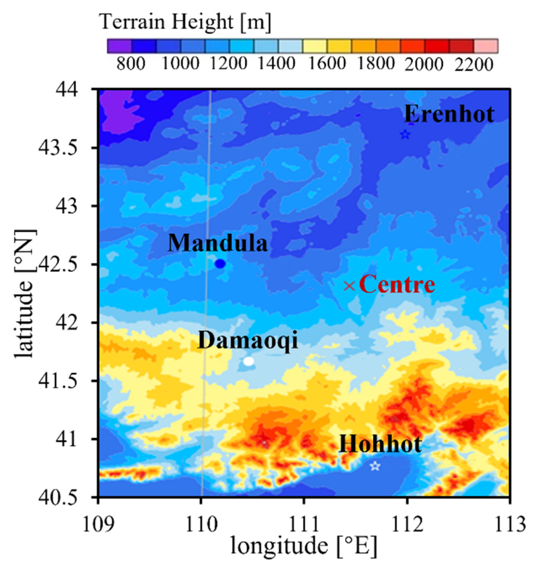
The results of the WRF model are compared to observations from the surroundings of the landing center, including data collected from the Erenhot and Hohhot radio-sounding stations, as well as from the Mandula and Damaoqi weather stations. The respective position coordinates of the four observation stations are shown in Table 2. The terrain height map of the main landing field and these four observation stations and their geographical relationships are shown in Figure 2.

3. Results and Discussion

The landing of the “Shen Zhou” series spacecraft goes through several processes, where the phase with parachute deployment is the final stage [33]. When the main parachute is fully opened, usually at an altitude of about 7 km, the return capsule begins to float in the atmosphere. At this time, the influence of wind on the flight trajectory reaches its maximum. As a result, more interest is paid to precise wind field simulations below 7 km in the current work. The simulation results are analyzed and discussed as follows.

3.1. “Shen Zhou 6” Case

The simulation period of the “Shen Zhou 6” spacecraft is set from the 14th to the 17th of October 2005. Figure 3 compares basic meteorological parameters, atmospheric pressure and potential temperature, obtained from the WRF model and the Erenhot and Hohhot radio-sounding stations, at 00:00 LST (Local Standard Time) on 17 October 2005. It is worth noting that OBS are short for observations in the figure and all the same in the following part. It shows that the WRF simulations reproduce the vertical variation of atmospheric pressure and potential temperature within the altitude range from the surface to 7 km, with pretty good accuracy. From Figure 3, it can be seen that atmospheric pressure decreases with altitude. The higher the altitude, the faster the atmospheric pressure decreases. On the contrary, because the vertical temperature reduction rate of the atmosphere is smaller than the dry adiabatic temperature reduction rate, the potential temperature generally increases with altitude. The consistency between the WRF simulations and the observations of these two meteorological parameters guarantees the accuracy analysis for wind characteristics in the following part.
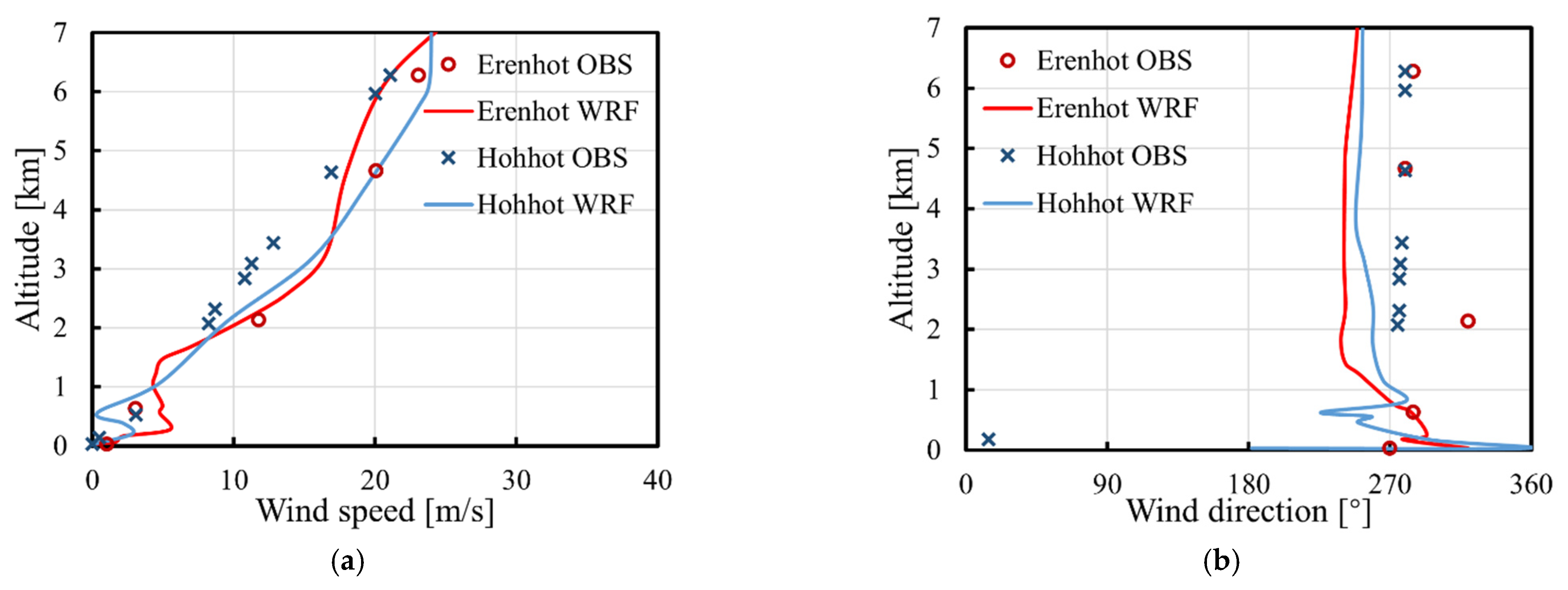
Figure 4 shows the distributions of wind speed and wind direction in the vertical direction at 00:00 LST on 17 October 2005. This shows that the WRF model can imitate wind behavior with acceptable accuracy. The profiles of wind speed and wind direction obtained by WRF and upper-level soundings have a remarkably similar trend. However, a noticeable deviation in wind direction is observed near the surface. Meanwhile, it is clearly shown that the wind direction profile at the higher altitude is much smoother than that at the lower altitude. As the altitude decreases, the profile shape seems more disturbed. This could be attributed to the fact that wind has distinct stratification characteristics at different altitudes.
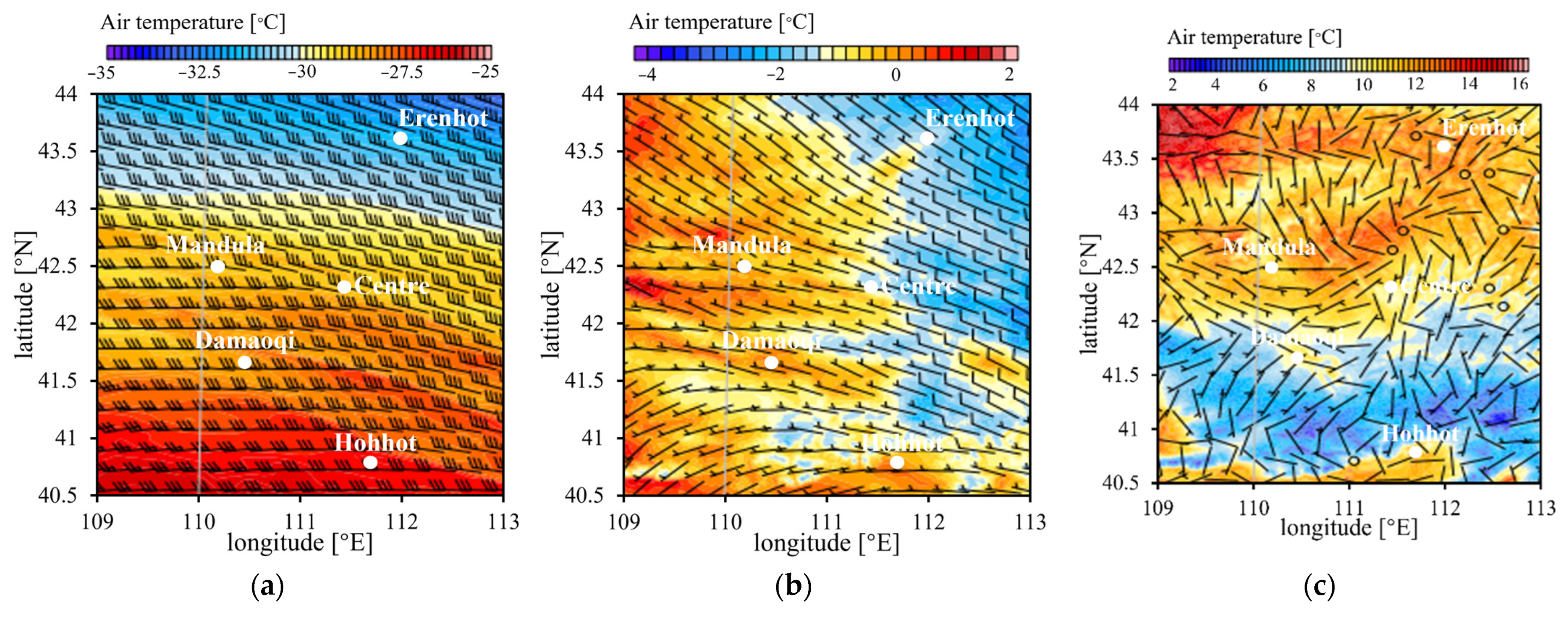
According to wind characteristics, wind fields below 7 km can be categorized into three altitude levels: free atmosphere layer (from 2 km to 7 km), Ekman layer (from 100 m to 2 km) and surface layer (from surface to 100 m). For a clear comparison of wind characteristics at different altitude layers, Figure 5 shows stratified wind vector maps at three typical altitudes.
The free atmosphere layer is far from the surface and not affected by surface friction, where the air movement follows the geostrophic wind or gradient wind law, with the wind direction almost unchanged, as shown in Figure 5a. With a decrease in altitude, the wind becomes sophisticated when entering the Ekman layer. Since surface friction, Coriolis force and pressure gradient work together here, wind direction changes are more obvious, as shown in Figure 5b. In the surface layer, turbulent viscosity is dominant. More affected by topography, the wind is relatively turbulent, which is reflected in Figure 5c, showing a random distribution of wind direction.
For the mean wind speed field, with upper-atmosphere sounding data as the reference, the statistical deviations obtained from the WRF forecasts are shown in Figure 6. The results are given every 12 h from 00:00 LST on 15 October to 12:00 LST on 17 October. Figure 6 shows that the absolute deviations are no more than 5 m/s. Specifically, deviations in Hohhot show more volatility, with a maximum value close to 10 m/s and a minimum value of about −5 m/s. In comparison, deviations between WRF and observations in Erenhot have a relatively more minor range, where the fluctuation range of the average relative wind speed error is almost controlled within ±12%.
Table 3 further shows the specific statistical biases of the mean wind speed for a more intuitive look. The results show that the average deviation is positive, meaning that the WRF forecasts are generally larger than the observations. Consistent with that shown in Figure 5, deviations are more minor in Erenhot than in Hohhot. In Erenhot, the absolute value of the average deviation does not exceed 2 m/s, while in Hohhot, the maximum absolute value of the average deviation is close to 4 m/s. Overall, the WRF model reproduces a wind speed field with reasonable accuracy.
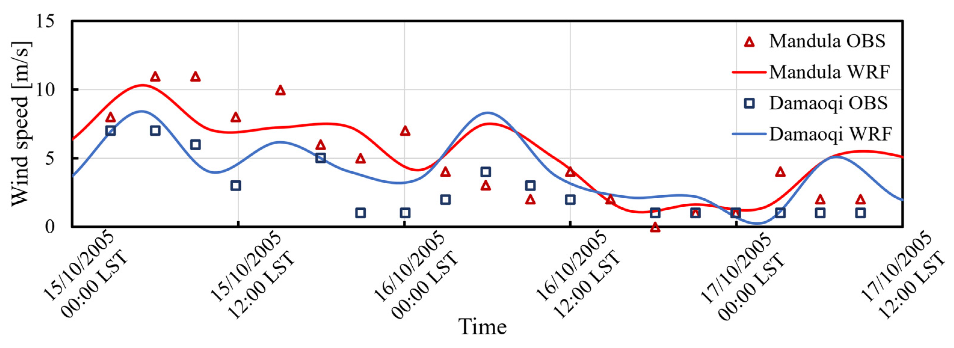
Since for airdrop and spacecraft recovery missions, precise flared landing near the ground is much of great importance. Figure 7 also shows a variation comparison of near-surface wind speed above the main landing area between the WRF and weather stations in the simulation period. It can be seen that the overall prediction of the near-surface wind field by the WRF model system is realistic. The variation in wind speed with time is well reproduced.

3.2. “Shen Zhou 7” Case

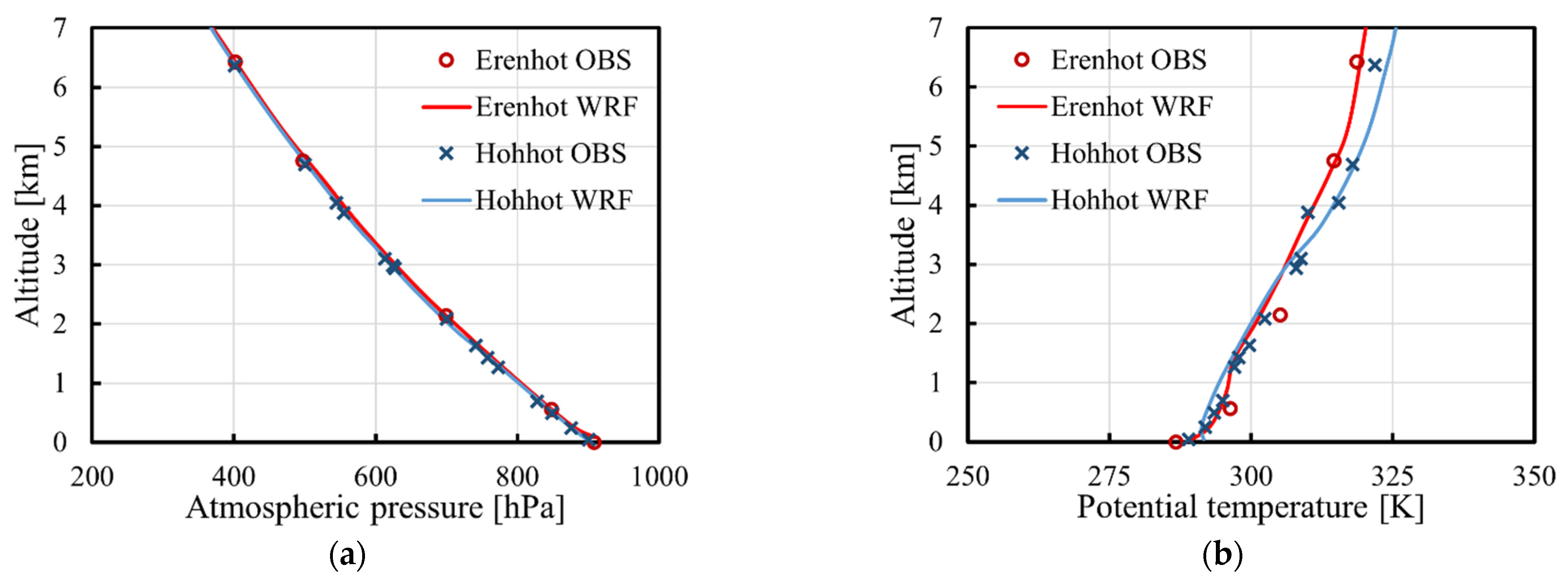
The simulation period, from the 26th to the 29th of September 2008, covers the whole landing phase of the “Shen Zhou 7” spacecraft with parachute. Figure 8 shows atmospheric pressure and potential temperature changes with altitude, obtained from the conventional upper-atmosphere sounding data and the WRF model at 00:00 LST on 28 September 2008.
Similar to Figure 3 in Section 3.1, Figure 8 shows that the WRF simulations reproduce the vertical variation of atmospheric pressure and potential temperature with pretty good accuracy. The consistency between the WRF simulations and the observations for basic meteorological parameters guarantees further accuracy analysis of wind characteristics.
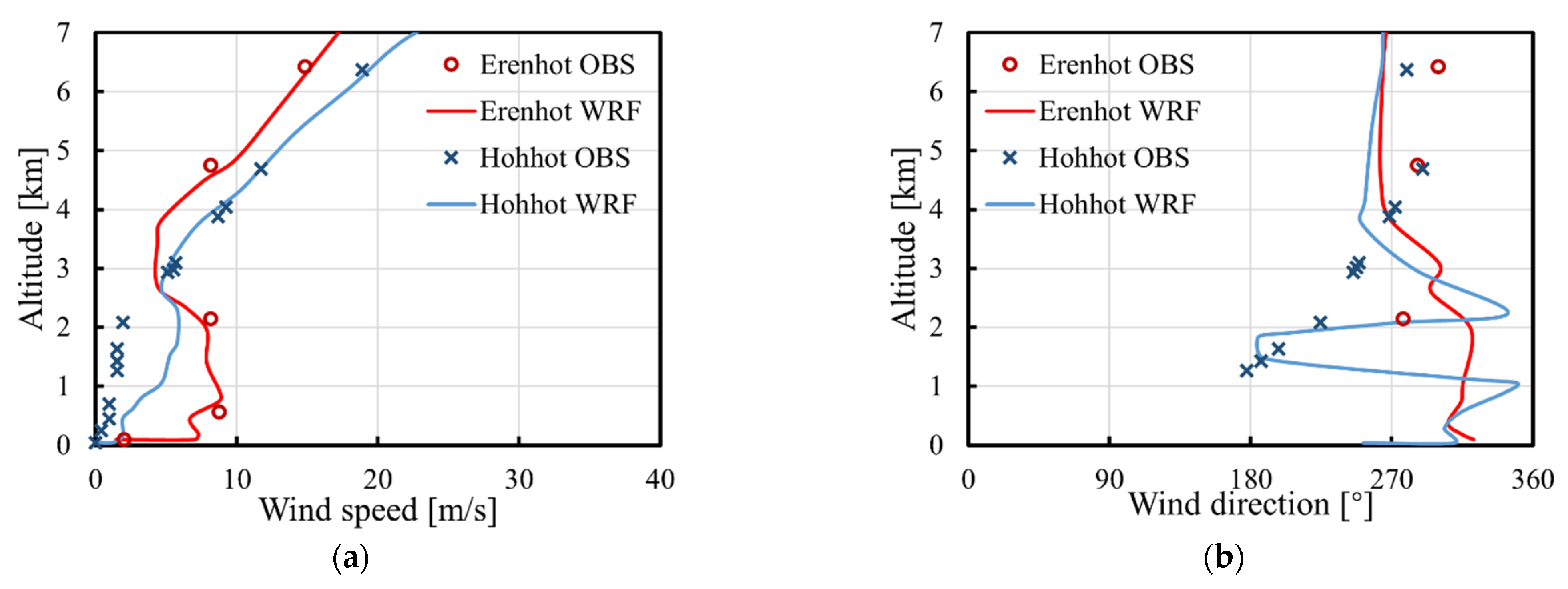
Figure 9 shows vertical wind speed and wind direction distributions above the main landing area at 00:00 LST on 28 September 2008. The results show that the WRF model can well imitate wind behavior on the whole. Specifically, the profile of the wind speed predicted by the WRF model system in Erenhot is in perfect agreement with the observations. In Hohhot, WRF forecasts in the altitude range of 3–7 km also agree well with the observed values. However, there are still apparent deviations from WRF predictions of wind direction. It shows significant fluctuations in wind direction predictions over Hohhot, which does not match the observation data. Considering that in the trajectory planning of the parafoil system, more interest is concentrated on the average wind speed, the overall WRF forecasts are acceptable.
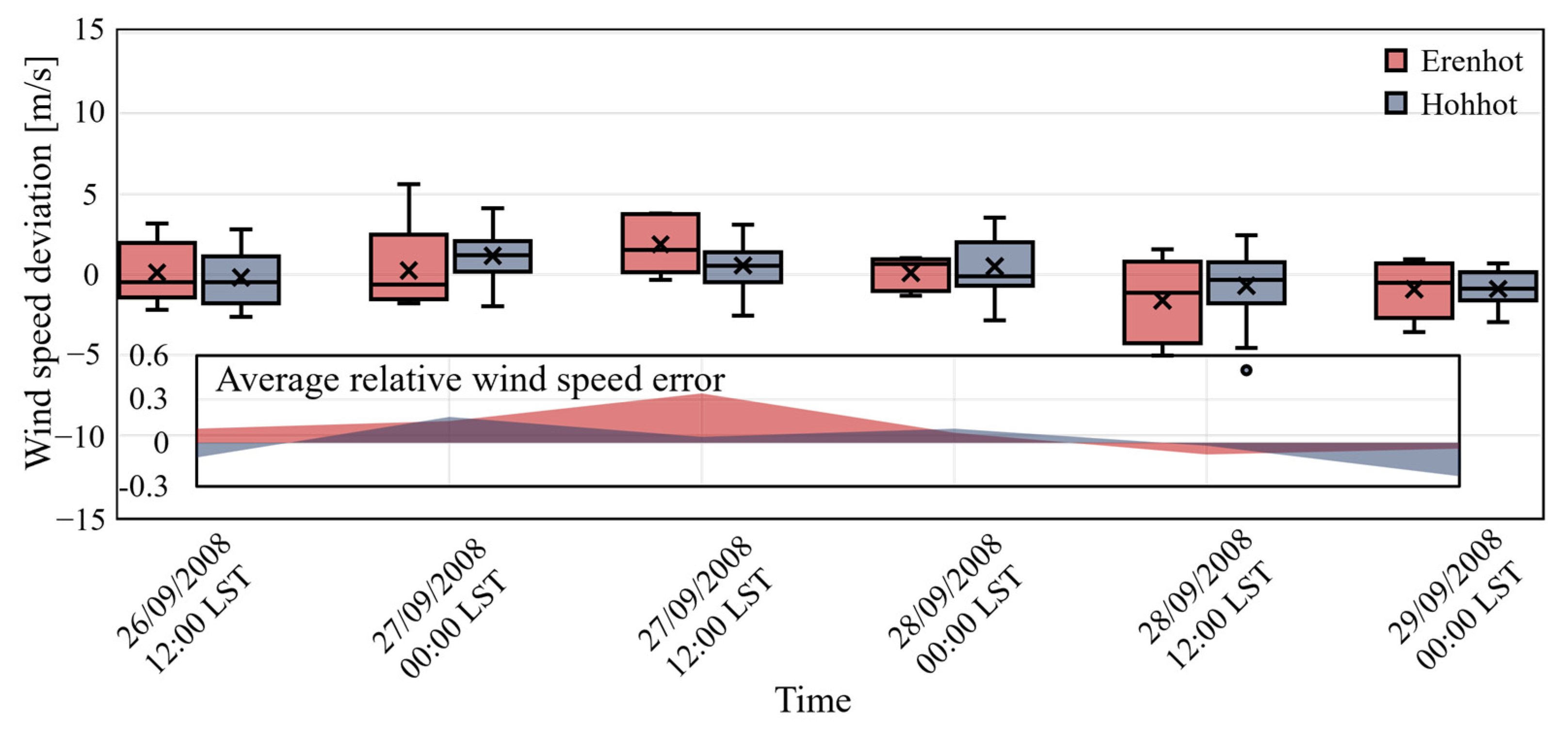
Figure 10 shows the statistical deviations obtained from the WRF forecasts, with upper atmosphere sounding data as the reference. Results are given every 12 h from 12:00 LST on 26 September to 00:00 LST on 29 September. Similar to Figure 6 in Section 3.1, it shows that absolute deviations almost fluctuate in the range of 5 m/s. The difference from Figure 6 is that, in this case, deviations in Hohhot are more concentrated than those in Erenhot.
Table 4 further shows the specific statistical biases of the mean wind speed. It can be seen that the average deviations are scattered around zero and have relatively small absolute values. The maximum absolute value of both average deviations in Erenhot and Hohhot does not exceed 2 m/s. In particular, average variations at 12:00 LST on 26 September 2008 are tiny; the absolute values are no more than 0.20 m/s.
With the results in Hohhot as an example, Table 5 shows relative wind speed error between WRF and upper-atmosphere sounding data obtained at 12:00 LST on 26 September 2008. Several feature points in the respective altitude ranges clearly show that the maximum relative wind speed error is controlled within 10%. The average absolute value of the relative wind speed error is only 4.52%. This means that the WRF model system can forecast well the wind speed field at all altitude layers.
To validate the wind speed forecasts near the surface, Figure 11 shows a near-surface wind speed variation comparison in the simulation period from 12:00 LST on 26 September 2008 to 00:00 LST on 29 September 2008 in this case. In comparison with Figure 7, in the “Shen Zhou 6” case, the overall wind speed near the surface is small, almost no more than 5 m/s. Under these circumstances, it is more difficult for WRF to capture the wind speed field precisely. From Figure 11, it can be seen that the WRF forecasts in Mandula are better than those in Damaoqi. In Mandula, wind disturbance and variation changes are well reproduced and consistent with observations. In contrast, relatively significant deviations occurred between WRF forecasts and observation data in Daomaoqi. However, since near-surface wind speed is rather low, the absolute value of deviations is also tiny, exhibiting less impact on a trajectory.

3.3. “Shen Zhou 10” Case

For the “Shen Zhou 10” spacecraft case, the simulation period is set from the 24th to the 27th of June 2013. Figure 12 gives the WRF forecasting profiles of the atmospheric pressure and potential temperature above the main landing area at 12:00 LST on 25 June 2013. Compared with the upper-atmosphere sounding data obtained from the Erenhot and Hohhot radio-sounding stations, WRF produces generally consistent results. This guarantees further accuracy analysis of wind characteristics.
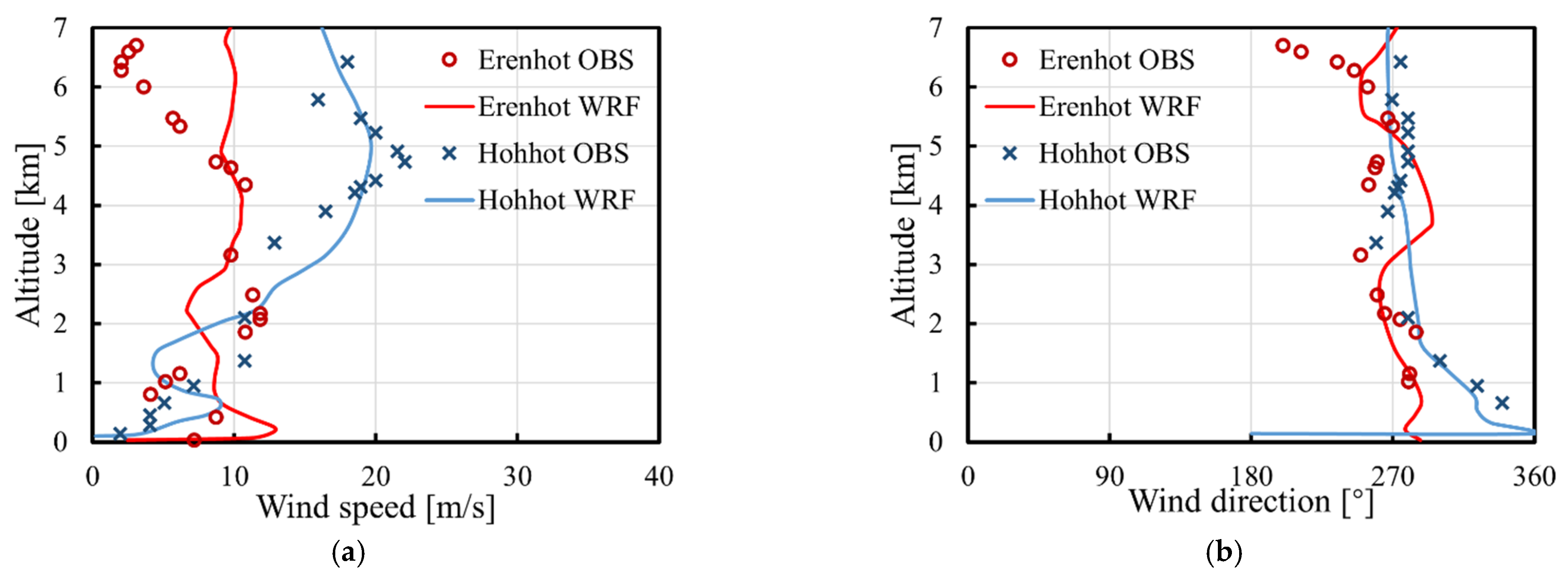
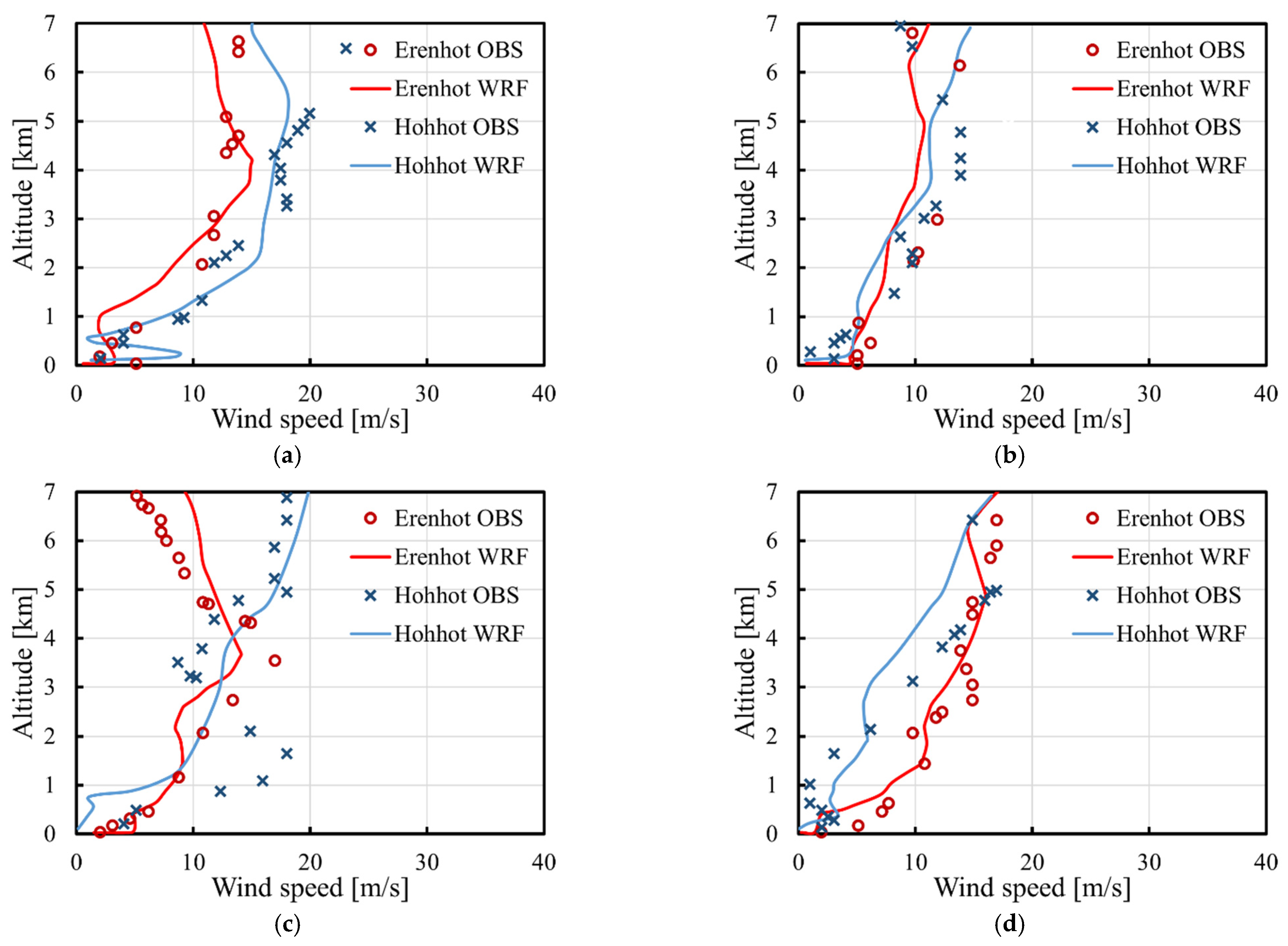
Figure 13 shows the vertical distributions of wind speed and wind direction above the main landing area at 12:00 LST on 25 June 2013. Unlike the above two cases, the WRF model is better at reproducing a changeable wind direction. In addition, compared with instances of “Shen Zhou 6” and “Shen Zhou 7,” wind speed profiles in the vertical direction differ in Erenhot and Hohhot, rather than a consistent trend.
To verify whether the inconsistency between wind speed profiles from two neighborhood radio-sounding stations is common or accidental, Figure 14 further shows profiles of the wind speed at the other four moments. It can be seen that the divergence in wind speed profiles is incidental. In combination with Figure 13a and Figure 14c, this is an occasional phenomenon on 25 June 2013. Most of the time, as seen in Figure 14a,b,d, the wind behaviors are generally consistent at both Erenhot and Hohhot.
With the removal of outliers, Table 6 shows the statistical biases of the mean wind speed. Compared with the above two cases, deviations fluctuate more, showing larger maximum and smaller minimum values. Nevertheless, the average variations are still scattered around zero and have small absolute values. The maximum absolute value of the average deviations in Erenhot is 2.77 m/s at 12:00 LST on 26 June 2013, and in Hohhot it is 2.42 m/s at 00:00 LST on 26 June 2013. At the other moments, the maximum absolute value in both Erenhot and Hohhot does not exceed 2 m/s. It demonstrates the relatively high reliability of the WRF results.
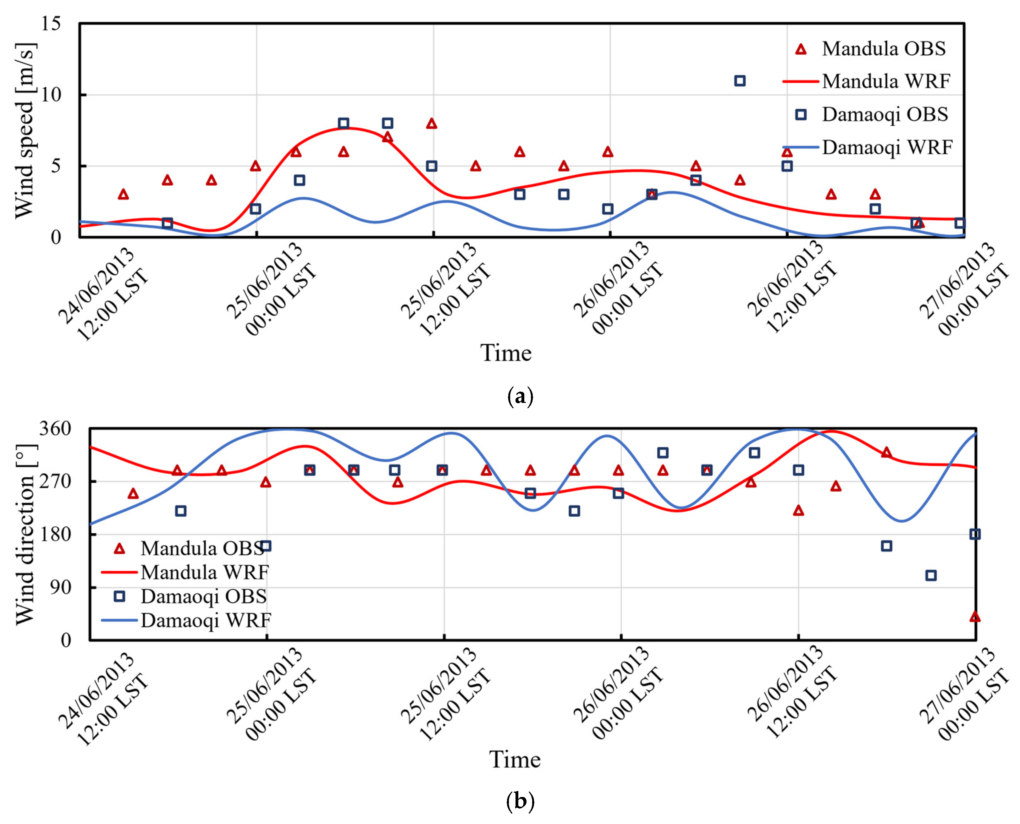
Figure 15 shows the variation of near-surface wind speed and wind direction above the main landing area obtained from WRF and weather stations from 12:00 LST on 24 June 2013 to 00:00 LST on 27 June 2013. It can be seen that the overall prediction of the near-surface wind field by the WRF model system is consistent with the observations. By comparison, the WRF forecasts in Mandula are better than those in Daomaoqi, which is similar to that concluded from the “Shen Zhou 7” case.

4. Engineering Wind Model

WRF model system is proven to provide a spatio-temporally varying wind field based on region and time with relatively good accuracy. In this section, further analysis of engineering wind models is done. A simplified wind model is built based on the WRF forecasting wind data from the above three cases. Validation is carried out on the simplified model using the observational wind properties in each case.
Assuming that the vertical wind v 3 = 0 , so the wind motion can be represented as
V w = ( V w h ,   0 ) ,
where V w h = ( v 1 , v 2 ) is the horizontal wind.
Introducing a horizontal wind speed function that varies linearly with height, the magnitude of the horizontal wind speed is given as:
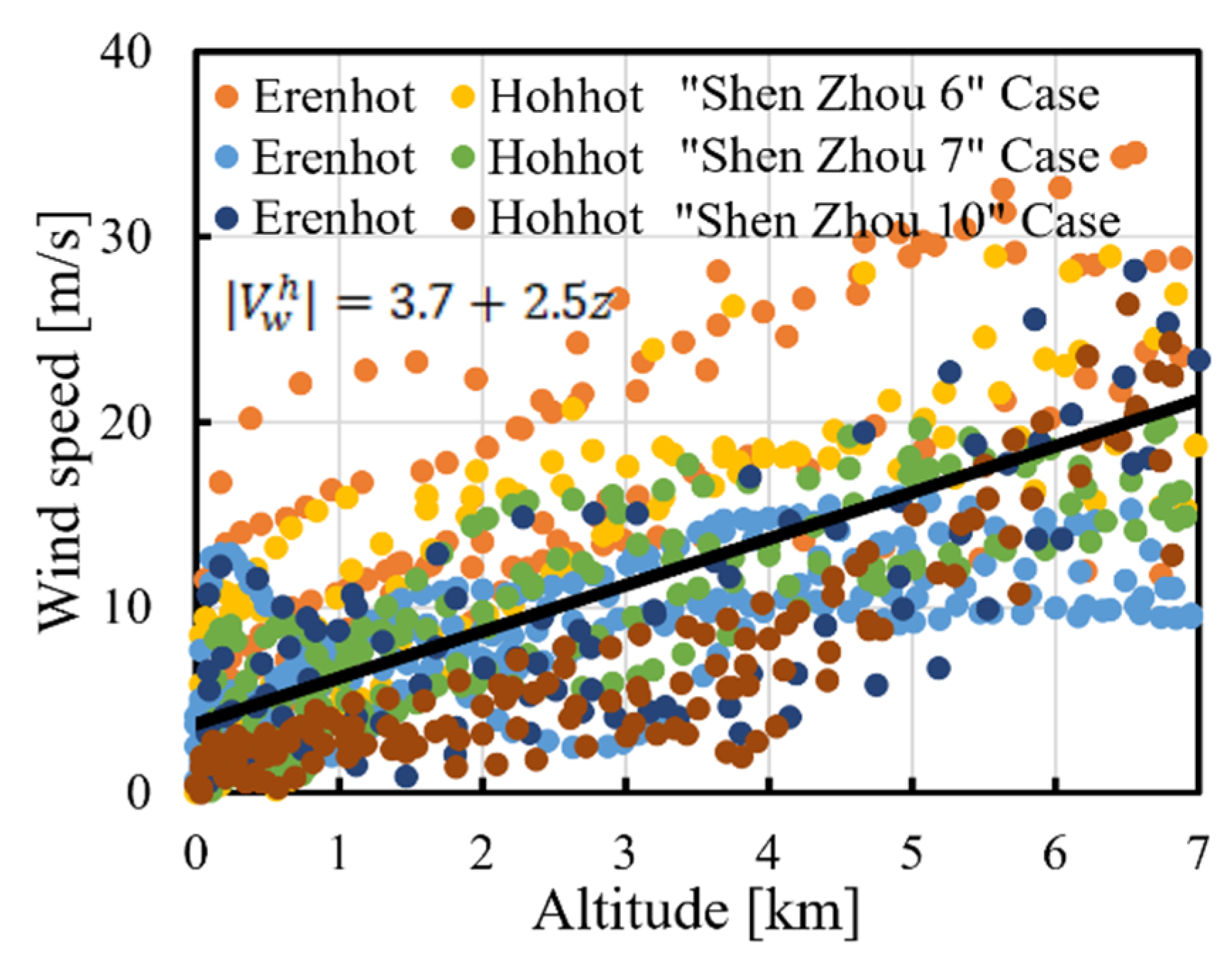
| V w h | = w 0 + a z ,
where w 0 is the near-surface wind speed, z is the altitude height.
The linear relationship described in Equation (2) has been fitted to the WRF forecast data from the above three cases, as shown in Figure 16. Using 18 independent WRF simulated z -profiles across surrounding locations (the Erenhot and Hohhot radio-sounding stations) of the landing center, typical w 0 and a values are found. It is clearly seen that w 0 = 3.7   m · s 1 and a = 2.5   s 1 can be used to approximate z -profiles constructed from WRF datasets.
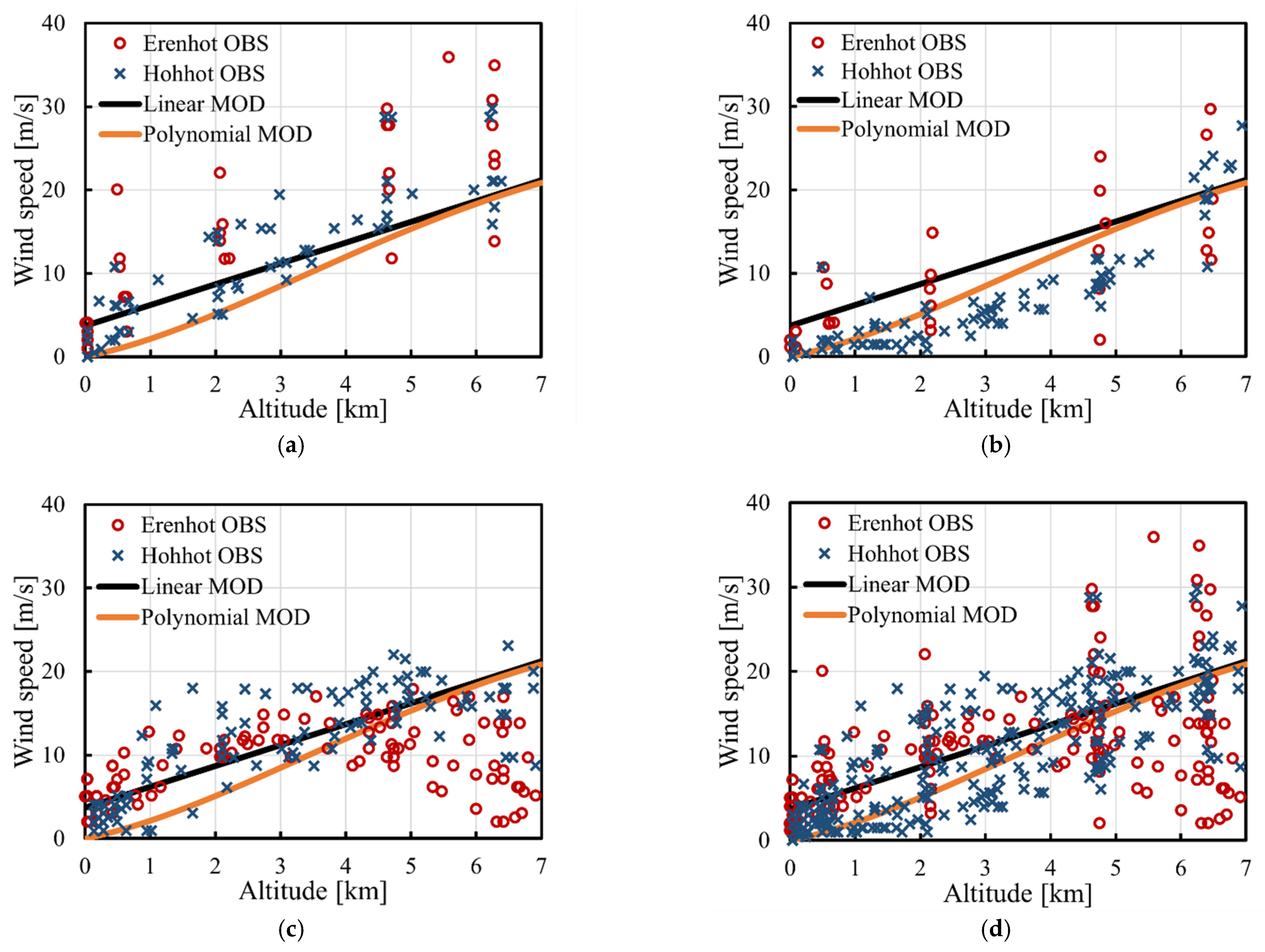
To validate the applicability and accuracy of the simplified model, observational wind properties from radio-sounding stations are used for comparison in Figure 17. In addition, a sixth-order polynomial model proposed by Cao [13] is also included for comparison. In Figure 17, MOD are abbreviations for models. The performance of these two models is examined by statistical parameters using R2 (coefcient of determination) and MSE (mean squared error). These parameters are calculated using Equations (3) and (4), shown as follows:
R 2 = 1 ( i = 1 n ( X A , i X P , i ) 2 i = 1 n X P , i 2 ) ,
M S E = 1 n i = 1 n ( X A , i X P , i ) 2 .
From the statistical analysis, it shows that the current proposed linear model performs better than the sixth-order polynomial model, with its predictions more identical to the observational data. The overall value of R2 for the proposed model is 0.71241, which is better than 0.64670 for the sixth-order polynomial model, since the closer R2 is to 1, the better the fitting effect is. In addition, the lowest values of MSE for the current proposed model and the sixth-order polynomial model are found to be 18.45828 and 22.67614, respectively. The smaller the value of the MSE, the more accurate the prediction effect.
Specifically, from Figure 17a,c, the polynomial model underestimates the wind speed below 4 km, as this altitude range is beyond its applicability. In this range, the proposed linear model shows more consistency with data obtained from radio-sounding stations. On the other hand, in the altitude range of 5 km–7 km, the two models have remarkably similar prediction trends. Considering that the polynomial model is proposed and validated based on the abundant observational high-altitude data, it can be concluded that the current model has good accuracy and reproduces the wind behaviors in this range well.

5. Summary and Conclusions

This study aims to evaluate the performance of the Weather Research Forecast (WRF) model in reproducing wind fields during the landing phase of the “Shen Zhou” series spacecraft mission. With suitable parameterization schemes and representative parameters for the landing site, simulations are carried out with three cases. They are the “Shen Zhou 6” case, the “Shen Zhou 7” case and the “Shen Zhou 10” case, respectively. The results are validated by comparison with observational data from the surrounding radio-sounding stations and weather stations. In terms of the vertical and horizontal distribution of wind speed, it proves that the WRF model has the ability to give a precise wind field at specific altitude layers.
Based on WRF forecasting wind data, a simplified linear wind model is proposed. Observational wind properties from radio-sounding stations are used for comparison to validate the applicability and accuracy of the linear model. This shows that the current proposed model has good consistency with observations. In addition, compared with a mature sixth-order polynomial model, it performs better at lower altitudes, especially below 4 km.
Through the current work, it can be concluded that the WRF model has the potential to provide an accurate imitation of wind behaviors. The proxy datasets generated by the WRF model not only help understand wind performance, but also complement the data sources for modeling the wind field. It is expected to be an alternative technique for costly and time-consuming experimental undertakings. Moreover, in comparison with the high-order polynomial model, the linear model is more suitable in the altitude range, specifically for parafoil trajectory planning.

Author Contributions

Conceptualization, Y.S. and L.T.; methodology, Y.S. and G.M.; software, Y.S. and G.M.; validation, Y.S.; formal analysis, G.M.; writing—original draft preparation, Y.S.; writing—review and editing, L.T. and G.M.; supervision, N.Z. and X.L. All authors have read and agreed to the published version of the manuscript.

Funding

This research was funded by the National Key Research and Development Program of China, grant number 2019YFE0192600, and the Fundamental Research Funds for the Central Universities, grant number NS2022010, and supported by the Priority Academic Program Development of Jiangsu Higher Education Institutions.

Institutional Review Board Statement

Not applicable.

Informed Consent Statement

Not applicable.

Data Availability Statement

Not applicable.

Conflicts of Interest

The authors declare no conflict of interest.

References

  1. Fortier, L.J. An Application of a Proposed Airdrop Planning System; Massachusetts Institute of Technology: Cambridge, MA, USA, 2004. [Google Scholar]
  2. Cinnamon, A. Improving Airdrop Precision Through Error Budget Analysis. In Proceedings of the Interservice/Industry Training, Simulation, and Education Conference, Orlando, FL, USA, 28 November–2 December 2016. [Google Scholar]
  3. Hasager, C.B.; Astrup, P.; Zhu, R.; Chang, R.; Badger, M.; Hahmann, A.N.J.R.S. Quarter-century offshore winds from SSM/I and WRF in the North Sea and South China Sea. Remote Sens. 2016, 8, 769. [Google Scholar] [CrossRef] [Green Version]
  4. Hasager, C.B.; Hahmann, A.N.; Ahsbahs, T.; Karagali, I.; Sile, T.; Badger, M.; Mann, J.J.W.E.S. Europe’s offshore winds assessed with synthetic aperture radar, ASCAT and WRF. Wind. Energy Sci. 2020, 5, 375–390. [Google Scholar] [CrossRef] [Green Version]
  5. Sward, J.; Ault, T.; Zhang, K.J.E. Spatial biases revealed by LiDAR in a multiphysics WRF ensemble designed for offshore wind. Energy 2023, 262, 125346. [Google Scholar] [CrossRef]
  6. Yuan, H.; Du, J.; Hou, J.J.J.o.t.M.S. The numerical simulation of wind fields in main landing-area by model WRF in the phase of “Shen Zhou 6” spacecraft mission. Sci. Meteorol. Sin. 2008, 28, 56–61. [Google Scholar]
  7. Guo, Z.; Miao, Q.; Wang, S.; Li, H.J.S.C.E.S. Prediction of the trajectory of the manned spacecraft SHENZHOU-7 deploying a parachute based on a fine wind field. Sci. China Earth Sci. 2011, 54, 1413–1429. [Google Scholar] [CrossRef]
  8. Magelinski, T. Uncertainty and Inaccuracy of Airdrop Modeling. Baccalaureate Thesis, Virginia Polytechnic and State University, Blacksburg, VA, USA, May 2017. [Google Scholar]
  9. Cañadillas, B.; Beckenbauer, M.; Trujillo, J.J.; Dörenkämper, M.; Foreman, R.; Neumann, T.; Lampert, A.J.W.E.S. Offshore wind farm cluster wakes as observed by long-range-scanning wind lidar measurements and mesoscale modeling. Wind. Energy Sci. 2022, 7, 1241–1262. [Google Scholar] [CrossRef]
  10. Kale, B.; Buckingham, S.; van Beeck, J.; Cuerva-Tejero, A.J.R.E. Implementation of a generalized actuator disk model into WRF v4. 3: A validation study for a real-scale wind turbine. Renew. Energy 2022, 197, 810–827. [Google Scholar] [CrossRef]
  11. Beal, T.R. Digital simulation of atmospheric turbulence for Dryden and von Karman models. J. Guid. Control. Dyn. 1993, 16, 132–138. [Google Scholar] [CrossRef]
  12. Vishniak, A. Simulation of the payload-parachute-wing system flight dynamics. In Proceedings of the Aerospace Design Conference, Melbourne, Australia, 13–15 September 1993; p. 1250. [Google Scholar]
  13. Cao, K. A Study of Fundamental Heat Transfer Behavior at Near-Space Altitudes; The University of Alabama: Tuscaloosa, AL, USA, 2008. [Google Scholar]
  14. Skamarock, W.C.; Klemp, J.B.; Dudhia, J.; Gill, D.O.; Liu, Z.; Berner, J.; Wang, W.; Powers, J.G.; Duda, M.G.; Barker, D. A Description of the Advanced Research WRF Model Version 4; National Center for Atmospheric Research: Boulder, CO, USA, 2019; Volume 145, p. 145. [Google Scholar]
  15. Kleczek, M.A.; Steeneveld, G.-J.; Holtslag, A.A.J.B.-L.M. Evaluation of the weather research and forecasting mesoscale model for GABLS3: Impact of boundary-layer schemes, boundary conditions and spin-up. Bound. Layer Meteorol. 2014, 152, 213–243. [Google Scholar] [CrossRef]
  16. Hahmann, A.N.; Vincent, C.L.; Peña, A.; Lange, J.; Hasager, C.B. Wind climate estimation using WRF model output: Method and model sensitivities over the sea. Int. J. Climatol. 2015, 35, 3422–3439. [Google Scholar] [CrossRef]
  17. Hassim, M.; Lane, T.; Grabowski, W. Physics. The diurnal cycle of rainfall over New Guinea in convection-permitting WRF simulations. Atmos. Chem. Phys. 2016, 16, 161–175. [Google Scholar] [CrossRef]
  18. Short, C.J.; Petch, J. Reducing the spin-up of a regional NWP system without data assimilation. Q. J. R. Meteorol. Soc. 2022, 148, 1623–1643. [Google Scholar] [CrossRef]
  19. Bowden, J.H.; Otte, T.L.; Nolte, C.G.; Otte, M.J. Examining interior grid nudging techniques using two-way nesting in the WRF model for regional climate modeling. J. Clim. 2012, 25, 2805–2823. [Google Scholar] [CrossRef]
  20. Muñoz-Sabater, J.; Dutra, E.; Agustí-Panareda, A.; Albergel, C.; Arduini, G.; Balsamo, G.; Boussetta, S.; Choulga, M.; Harrigan, S.; Hersbach, H.J. ERA5-Land: A state-of-the-art global reanalysis dataset for land applications. Earth Syst. Sci. Data 2021, 13, 4349–4383. [Google Scholar] [CrossRef]
  21. Kokaly, R.; Clark, R.; Swayze, G.; Livo, K.; Hoefen, T.; Pearson, N.; Wise, R.; Benzel, W.; Lowers, H.; Driscoll, R.J. Usgs Spectral Library Version 7 Data: Us Geological Survey Data Release; United States Geological Survey (USGS): Reston, VA, USA, 2017.
  22. Hong, S.-Y.; Lim, J.-O.J. The WRF single-moment 6-class microphysics scheme (WSM6). Asia-Pac. J. Atmos. Sci. 2006, 42, 129–151. [Google Scholar]
  23. Mlawer, E.J.; Taubman, S.J.; Brown, P.D.; Iacono, M.J.; Clough, S.A. Radiative transfer for inhomogeneous atmospheres: RRTM, a validated correlated-k model for the longwave. J. Geophys. Res. Atmos. 1997, 102, 16663–16682. [Google Scholar] [CrossRef] [Green Version]
  24. Ruiz-Arias, J.A.; Dudhia, J.; Santos-Alamillos, F.J.; Pozo-Vázquez, D. Surface clear-sky shortwave radiative closure intercomparisons in the Weather Research and Forecasting model. J. Geophys. Res. Atmos. 2013, 118, 9901–9913. [Google Scholar] [CrossRef]
  25. Dudhia, J. Numerical study of convection observed during the winter monsoon experiment using a mesoscale two-dimensional model. J. Atmos. Sci. 1989, 46, 3077–3107. [Google Scholar] [CrossRef]
  26. Hari Prasad, K.; Venkata Srinivas, C.; Venkateswara Naidu, C.; Baskaran, R.; Venkatraman, B. Assessment of surface layer parameterizations in ARW using micro-meteorological observations from a tropical station. Meteorol. Appl. 2016, 23, 191–208. [Google Scholar] [CrossRef] [Green Version]
  27. Janjic, Z.I. The surface layer in the NCEP Eta Model. In Proceedings of the Eleventh Conference on Numerical Weather Prediction, Norfolk, VA, USA, 19–23 August 1996; American Meteorological Society: Boston, MA, USA; pp. 354–355. [Google Scholar]
  28. Janić, Z.I. Nonsingular Implementation of the Mellor-Yamada Level 2.5 Scheme in the NCEP Meso Model; National Centers for Environmental Prediction (U.S.): College Park, MD, USA, 2001.
  29. LeMone, M.A.; Tewari, M.; Chen, F.; Alfieri, J.G.; Niyogi, D. Evaluation of the Noah land surface model using data from a fair-weather IHOP_2002 day with heterogeneous surface fluxes. Mon. Weather. Rev. 2008, 136, 4915–4941. [Google Scholar] [CrossRef]
  30. Nakanishi, M.; Niino, H. Development of an improved turbulence closure model for the atmospheric boundary layer. J. Meteorol. Soc. Jpn. 2009, 87, 895–912. [Google Scholar] [CrossRef] [Green Version]
  31. Kain, J.S.; Fritsch, J.M. Convective parameterization for mesoscale models: The Kain-Fritsch scheme. In The Representation of Cumulus Convection in Numerical Models; Springer: Berlin/Heidelberg, Germany, 1993; pp. 165–170. [Google Scholar]
  32. Kain, J.S. The Kain–Fritsch convective parameterization: An update. J. Appl. Meteorol. 2004, 43, 170–181. [Google Scholar] [CrossRef]
  33. Albiñana Burdiel, C. Design and Testing of a Parachute Recovery System for a Sounding Rocket Experiment; Universitat Politècnica de València: Valencia, Spain, 2022. [Google Scholar]
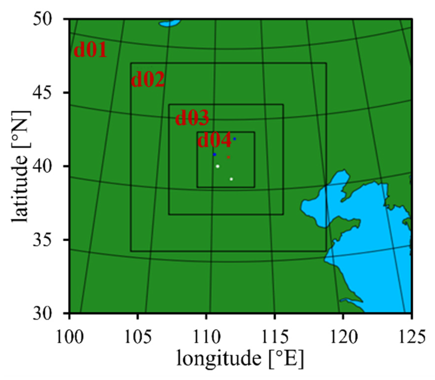
Figure 1. Geographical fourfold-nested domain covered by the WRF model.
Aerospace 10 00037 g001
Figure 2. Terrain height map of the main landing field and its surroundings.
Aerospace 10 00037 g002
Figure 3. Profiles of (a) atmospheric pressure and (b) potential temperature above the main landing area from WRF and observations at 00:00 LST on 17 October 2005.
Aerospace 10 00037 g003
Figure 4. Profiles of (a) wind speed and (b) wind direction above the main landing area from WRF and upper-atmosphere sounding data at 00:00 LST on 17 October 2005.
Aerospace 10 00037 g004
Figure 5. Stratified wind vector maps at altitudes of about (a) 6700 m, (b) 2000 m and (c) 15 m, respectively.
Aerospace 10 00037 g005
Figure 6. Statistical deviations of mean wind speed field obtained from WRF forecasts in the “Shen Zhou 6” case.
Aerospace 10 00037 g006
Figure 7. Variation of near-surface wind speed above the main landing area from WRF and weather stations from 00:00 LST on 15 October 2005 to 12:00 LST on 17 October 2005.
Aerospace 10 00037 g007
Figure 8. Profiles of (a) atmospheric pressure and (b) potential temperature above the main landing area from WRF and upper-atmosphere sounding data at 00:00 LST on 28 September 2008.
Aerospace 10 00037 g008
Figure 9. Profiles of (a) wind speed and (b) wind direction above the main landing area from WRF and upper-atmosphere sounding data at 00:00 LST on 28 September 2008.
Aerospace 10 00037 g009
Figure 10. Statistical deviations of mean wind speed field obtained from WRF forecasts in the “Shen Zhou 7” case.
Aerospace 10 00037 g010
Figure 11. Variation of near-surface wind speed above the main landing area from WRF and weather stations from 12:00 LST on 26 September 2008 to 00:00 LST on 29 September 2008.
Aerospace 10 00037 g011
Figure 12. Profiles of (a) atmospheric pressure and (b) potential temperature above the main landing area from WRF and upper-atmosphere sounding data at 12:00 LST on 25 June 2013.
Aerospace 10 00037 g012
Figure 13. Profiles of (a) wind speed and (b) wind direction above the main landing area from WRF and upper-atmosphere sounding data at 12:00 LST on 25 June 2013.
Aerospace 10 00037 g013
Figure 14. Profiles of the wind speed above the main landing area from WRF and upper-atmosphere sounding data at (a) 12:00 LST on 24 June 2013, (b) 12:00 LST on 26 June 2013, (c) 00:00 LST on 25 June 2013 and (d) 00:00 LST on 27 June 2013.
Aerospace 10 00037 g014
Figure 15. Variation of near-surface (a) wind speed and (b) wind direction above the main landing area from WRF and weather stations from 12:00 LST on 24 June 2013 to 00:00 LST on 27 June 2013.
Aerospace 10 00037 g015
Figure 16. WRF forecasts data used to create linear approximations of how wind speed varies with height.
Aerospace 10 00037 g016
Figure 17. Comparison of modeled and observed wind fields above the main landing area in the (a) “Shen Zhou 6” case, (b) “Shen Zhou 7” case, (c) “Shen Zhou 10” case, and (d) the whole case, including the above three cases.
Aerospace 10 00037 g017
Table 1. Physical configuration used in the simulation.
Physical ProcessParameterization Scheme
MicrophysicsWSM6 (WRF Single-moment 6-class) [22]
Longwave radiationRRTM (Rapid Radiative Transfer Model) [23]
Shortwave radiationDudhia [24,25]
Surface layerEta similarity (Monin-Obukhov) [26,27,28]
Land surfaceNoah [29]
PBL physicsMYNN (Mellor-Yamada-Nakanishi-Niino) 2.5 level TKE [30]
Cumulus physicsKain-Fritsch (new Eta) [31,32]
Table 2. The respective position coordinates of the four observation stations.
Station NameStation No.Longitude [°E]Latitude [°N]Altitude [m]
Mandula53,14942.533110.1331223
Damaoqi53,35241.700110.4331377
Erenhot53,06843.650112.000996
Hohhot53,46340.810111.6801065
Table 3. Statistical biases of mean wind speed above the main landing area in the “Shen Zhou 6” case.
Time [LST]Wind Speed [m/s]Time [LST]Wind Speed [m/s]
Maximum
Deviation
Minimum
Deviation
Average
Deviation
Maximum
Deviation
Minimum
Deviation
Average
Deviation
Erenhot Hohhot
15—00:003.84−2.051.8215—00:003.87−1.410.95
15—12:003.45−0.710.5915—12:002.620.881.18
16—00:003.57−2.260.7416—00:009.09−0.923.04
16—12:000.92−2.44−1.0616—12:003.015.633.83
17—00:00−2.171.86−0.8517—00:00−2.643.871.87
17—12:00−1.982.520.1317—12:00−1.373.791.25
Table 4. Statistical biases of mean wind speed above the main landing area in the “Shen Zhou 7” case.
Time [LST]Wind Speed [m/s]Time [LST]Wind Speed [m/s]
Maximum
Deviation
Minimum
Deviation
Average
Deviation
Maximum
Deviation
Minimum
Deviation
Average
Deviation
Erenhot Hohhot
26—12:003.17−2.170.1226—12:002.82−2.65−0.20
27—00:005.61−1.800.2627—00:004.13−1.991.17
27—12:003.75−0.331.8627—12:003.11−2.570.56
28—00:000.95−1.300.1028—00:003.54−2.860.50
28—12:001.55−5.03−1.6128—12:002.45−4.54−0.70
29—00:000.95−3.59−0.9129—00:000.67−2.94−0.90
Table 5. Relative wind speed error between WRF and upper-atmosphere sounding data obtained in Hohhot at 12:00 LST on 26 September 2008.
Layer NameAltitude RangeNo.Altitude [m]Relative Wind Speed Error [%]
Free atmosphere layer2 km–7 km16717.233.29
23817.233.30
32087.234.51
Ekman layer100 m–2 km41019.23−5.32
Surface layersurface–100 m512.236.17
The average absolute value of relative wind speed error [%]4.52
Table 6. Statistical biases of mean wind speed above the main landing area in the “Shen Zhou 10” case.
Time [LST]Wind Speed [m/s]Time [LST]Wind Speed [m/s]
Maximum
Deviation
Minimum
Deviation
Average
Deviation
Maximum
Deviation
Minimum
Deviation
Average
Deviation
Erenhot Hohhot
24—12:001.83−3.23−0.8324—12:002.88−1.79−0.62
25—00:004.46−3.650.8725—00:003.89−8.39−0.96
25—12:007.94−5.131.8325—12:004.69−6.480.00
26—00:006.99−6.620.0926—00:000.41−6.57−2.42
26—12:001.05−7.37−2.7726—12:006.03−2.570.06
27—00:001.05−4.73−1.6627—00:002.17−4.56−1.10
Disclaimer/Publisher’s Note: The statements, opinions and data contained in all publications are solely those of the individual author(s) and contributor(s) and not of MDPI and/or the editor(s). MDPI and/or the editor(s) disclaim responsibility for any injury to people or property resulting from any ideas, methods, instructions or products referred to in the content.