Abstract
Obtaining the inertia tensors of defunct space objects is essential in on-orbit missions. When the inertia tensor of the space object is non-diagonal, the problem becomes challenging. In this case, the system does not have enough information to estimate the six independent parameters of the inertia tensor. In this paper, the problem of estimating the inertial parameters of a defunct space object with non-diagonal inertia tensor is studied. An excitation method of ejecting an impact ball from the tracking spacecraft to the object is proposed to estimate the complete inertial parameters of the object. The impact ball rebounds after colliding with the object and crashes into the atmosphere finally. After the collision, the angular momentum of the space object changes. The change is used to construct the estimation model. This paper designs an estimation model which consists of two Unscented Kalman-based estimators to estimate the inertial parameters and the motion states of the object. The observability of the estimators is proved through the observability theorem of nonlinear systems. Numerical simulations show that the estimation model is effective in estimating the complete inertial parameters of defunct objects, as well as reducing the measurement errors of the position and attitude of the object.
1. Introduction
In certain on-orbit operation missions such as capturing defunct objects, the attitude and orbit motions of the spacecraft will be affected by the object [1]. A strong impact could damage the operating spacecraft. In this kind of mission, it is crucial to obtain knowledge of the inertial parameters of the defunct object [2,3]. The identification of the inertial parameters of defunct space objects has been one of the key technologies for on-orbit service of defunct objects. Identification methods of the inertial parameters of space objects can be divided into kinematics-based methods and dynamics-based methods. These two methods have the same characteristic in building a nonlinear identification model. Due to the inevitable influence of external interference and internal factors, the measurement errors of the measurement system will directly affect the identification accuracy of the inertial parameters. So in identifying of the inertial parameters, the measured values and the inertial parameters are considered together as the state variables to be estimated. It means the identification model is constructed to estimate the motion states and inertia characteristics of the object at the same time.
There are many publications on the inertial parameters identification of defunct space objects. Philip et al. [4] proposed an algorithm to estimate the moment of inertia of the object at the assumption that the defunct object is known with some cooperative characteristic points. Lichter et al. [5] designed a Kalman filter-based estimation algorithm to estimate the standard diagonal inertia tensor of the object. Wilson et al. [6,7] proposed a least squares-based identification model to identify the inertia tensors of defunct objects on the assumption that the estimated mass characteristics of the object are known. Sheinfeld et al. [8] estimated the proportional values between the inertial parameters. Benninghoff et al. [9] proposed an algorithm to identify the center of mass and moments of inertia of defunct objects based on least square estimation. However, all parameters of this algorithm can only be obtained under the condition that the object only has nutation. Pesce et al. [10] obtained the ratio of the moment of inertia and the relative position of the object. Yuan et al. [11,12] proposed a Kalman filter-based algorithm to estimate the ratio of the moments of inertia of defunct objects. Alessia et al. [13,14] used the LIDAR-based pose measurements to estimate the moment of inertia ratios of the object.
Without direct or indirect contact, the inertia tensors of defunct space objects can not be completely identified only by visual measurement [15,16]. To fully identify the inertial parameters of the object, the excitation information can be increased by actively changing the motion state of the defunct object. Murotsu et al. [17,18,19,20] proposed the estimation algorithms based on momentum conservation to identify the inertial parameters of the combination of the object and the tracking spacecraft after capturing the object. Leonard et al. [21] identified the center of mass and the inertial parameters of defunct objects by applying control torque to the object directly. Meng et al. [22,23] put forward the idea of directly contacting the object with a flexible rod or indirectly contacting the object with eddy current and magnetic field. By changing the motion state of the object through contact, the excitation information is increased. As a result, the complete inertial parameters of defunct objects are identified. Liu et al. [24] estimated the inertia parameters of the object by contacting softly with the noncooperative object.
In this paper, the problem of estimating the complete inertial parameters of defunct space objects is studied when the inertia tensor of the object is not diagonal. To estimate the inertial parameters of defunct space objects, we proposed a moment-excitation method to increase incentive information in reference [25]. By ejecting an impact ball from the tracking spacecraft towards the defunct object, the motion state of the object is changed. The change of the angular momentum of the object is utilized to construct the estimation model. In [25], the impact ball is assumed to adhere to the surface of the defunct object after the collision. The impact and adhesion mechanism of the impact ball are analyzed in [26]. As a further study based on references [25,26], this paper investigates the problem of estimating the complete inertial parameters of the object with non-diagonal inertia tensor. An impact-rebound-based estimation model is proposed while the impact-rebound happens between the impact ball and the object. The estimation model consists of two estimators, one is used to filter the measurement errors of the attitude and the position of the object, and the other is used to estimate the complete inertial parameters of the object. The observability of the estimation model will be proved theoretically.
This paper is organized as follows: Section 2 analyzes the problem and introduces the motion models of the object. Section 3 describes the state equation and observation equation of the estimation model. The observability of the estimation model is proved in Section 4. Numerical simulations are described in Section 5. Section 6 presents the conclusion.
2. Problem Analysis and System Modeling
In this paper, the problem of estimating the inertial parameters of defunct space objects is studied when the inertia tensor of the object is not diagonal. At this time, there are six inertial parameters of defunct objects. According to references [15,16], the six inertial parameters cannot be completely identified without additional excitation. In this paper, an impact-rebound based estimation model is proposed to estimate the inertial parameters of defunct objects based on references [25,26].
Figure 1 shows the schematic diagram of the collision between the impact ball and the defunct space object. The impact ball is ejected from the tracking spacecraft towards the defunct object. Then the ball collides with the object. As proved in reference [26], the relative velocity of the ball should be controlled to less than m/s to make sure that the object will not be punctured by the collision between the ball and the object. In addition, the impact ball should collide with the object eccentrically. In this situation, the angular momentum of the space object is changed by the collision. As the tracking spacecraft is close to the object, the influence of gravity gradient can be ignored. In addition, it is assumed that the defunct space object experiences no external torque except the collision between the impact ball and the object. Thus the angular momentum of the system consisting of the impact ball and the object is conserved. The motion states of the object and the impact ball are obtained through the measurement system installed on the tracking spacecraft. It should be noted that this paper focuses on the parameter estimation of the defunct object. The attitude and the position of the defunct object are provided by the measurement system. The problem in this paper can be summarized as follows. Based on the measurements of the state of the space object and the impact ball, an estimation model is designed to estimate the inertial parameters of the defunct object, as well as filtering the errors of the motion state measurements of the object.
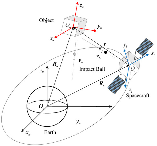
Figure 1.
The schematic diagram of the collision between the object and the impact ball.
2.1. Coordinate Frames
At first, the coordinate frames used in the paper are introduced. This paper concerns three objects: the tracking spacecraft, the defunct space object and the impact ball. Three coordinate frames are introduced to describe the motion state: the geocentric equatorial inertial coordinate frame , the local-vertical, local-horizontal Euler–Hill (LVLH) coordinate frame , and the body coordinate frame of the defunct object . The coordinate frames are shown in Figure 1. The origin of the inertial frame is defined at the center of Earth. The axis points to the direction of the vernal equinox. The axis is the spin axis of the Earth. The axis , axis , and axis form a right-handed orthogonal coordinate frame. The origin of the LVLH frame is defined at the center of mass of the tracking spacecraft. The axis coincides with the position vector of the spacecraft and points from the center of mass of Earth to the spacecraft. is perpendicular to the axis , and is defined in the orbit plane of the tracking spacecraft. The positive direction of is along with the direction of the velocity of the tracking spacecraft. The axis forms a right-handed system with the and . The frame is originated at the center of mass of the defunct object. When the three axes of the frame are aligned along the principal inertial axes, the inertia tensor of the object is diagonal. In this paper, the parameter estimation model is designed for the space objects with non-diagonal inertia tensors. The three axes of are not aligned along the principal inertial axes.
The attitude motion equation and the orbit motion equation of the space object are presented in the following context.
2.2. Attitude Motion
This section introduces the attitude motion equation of the object. In this paper, the (3-1-2) successive rotation Euler angle is selected to describe the attitude of the object relative to the inertial frame . The Euler angles of the object is defined as: . is introduced to represent the angular velocity of the object in the body coordinate frame relative to the inertial frame . The attitude kinematics equations are given by [27]:
where represent the acceleration of the Euler angles .
Euler’s dynamics equation is written as:
where is the inertia tensor of the object. is defined as:
where are the six independent parameters of the inertial tensor . Assuming that the object is rigid, the derivatives of the inertial parameters are zeros:
and is the total external torque applied in the object. It is assumed that the defunct space object experiences no control force or torque, so in this paper.
2.3. Orbit Motion
In this section, the relative motion equations of the object in LVLH frame are introduced. The schematic diagram of the relative motion of the tracking spacecraft and the defunct object is shown in Figure 2. The positions of the tracking spacecraft and the object in the inertial frame are noted as and . The relative position of the object in LVLH frame is defined as . Assuming that the orbit of the tracking spacecraft is circular, the acceleration of the angular velocity of the tracking spacecraft is zero. , the angular velocity of frame with respect to , is written as:
where is the average orbital angular velocity of the tracking spacecraft. is given by:
where is the modulus of , and represents the gravitational constant of the Earth.
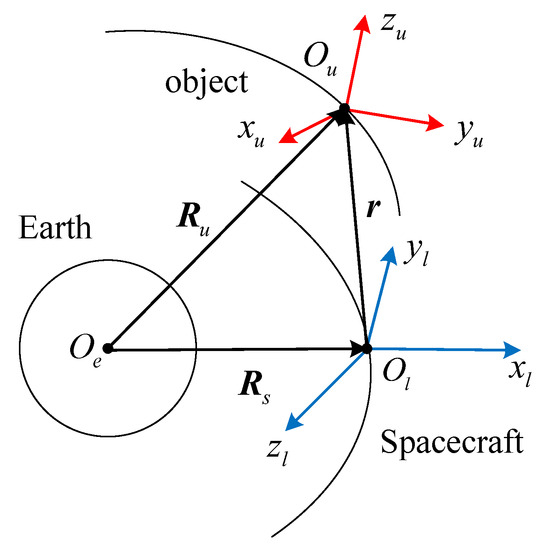
Figure 2.
The relative motion of the tracking spacecraft and the object.
The Clohessy–Wiltshire equations are used to describe a simplified model of the relative motion state of the object in LVLH frame [27]:
where is the relative velocity of the object in LVLH frame , and is the relative acceleration of the object in LVLH frame .
A state vector composed of the relative position and the relative velocity of the object is defined as: . According to Equation (10), the state equation of is:
where and are defined as:
As a conclusion, Equation (10) represents the relative motion equation of the object in LVLH frame . The relative position and the relative velocity of the object are updated by Equations (12) and (13).
As seen from the above theoretical analysis, the attitude and position of the object are updated by the attitude motion equation and the orbit motion equation. The core problem of updating the motion state is that the inertia tensor of the object in attitude dynamics equation (Equation (2)) is unknown. The inertial parameters of the object cannot be completely identified solely relying on vision. In this paper, an impact-rebound momentum excitation method is designed to estimate the six inertial parameters of the object. Since the system consisting of the impact ball and the object is free from any external force, the system follows the law of angular momentum conservation after the collision. After ejecting the impact ball, an autonomous control mechanism is introduced to compensate the reaction force of the impact ball on the tracking spacecraft. The relative motion of the spacecraft is still in the original orbit after ejecting the impact ball.
3. Parameter Estimation Filter Design
The attitude motion equations and the orbit motion equations of the defunct object are introduced in the last section. In this section, a parameter estimation model based on the Kalman filter algorithm is designed to estimate the motion state and the inertial parameters of the object. It should be noted that this paper focuses on the problem of estimating the inertial parameters of the object based on the measurements of the motion state. The Euler angles and the relative position of the object are provided by the measurement system installed on the tracking spacecraft. In the simulations, the measurements are set as the sum of the simulated values and noise signals.
The state vector of the parameter estimation model includes the Euler angles, the angular velocity, the relative position, the relative velocity and the inertial parameters of the object. is written as:
where represents the Euler angles and the angular velocity of the object, represents the relative position and the relative velocity of the object, is a vector composed of the inertial parameters of the object.
According to the expression of the state vector in Equation (14), the state equation of the estimation model is expressed as:
where is defined by Equation (5), and is defined by Equation (11). is the derivatives of the inertial parameters of the object. Under the assumption that the object is rigid, the derivatives of the inertial parameters are zeros. The expression of is presented as:
The general observation equation is written as:
where is the vector of the measurement data. describes the relationship between the state vector and the measurement data. represents the noise in the measurements. To completely estimate the inertial parameters of the defunct object, three sets of observation equations are established in this paper: two observation equations based on measurements and an observation equation based on angular momentum conservation model. The former two observation equations provide the measurement information about the Euler angles and the relative position of the object, which are widely used in filtering the motion state of the object. The latter observation equation is the core observation equation in this paper, which is obtained by the law of angular momentum conservation. The specific expressions and meanings of the three observation equations will be given in the following.
3.1. Observation Equations Based on Measurements
As mentioned in the previous section, the observation equations are composed of two parts: the measurements-based equations and the angular momentum conservation-based equations. This section introduce the measurements based equations. The measurements based equations include the Euler angles’ measurements and the relative position measurements.
The measurements of the Euler angles of the object are noted as . Define as:
Substituting Equation (18) into Equation (17), yields the expression of :
where means a identity matrix, and represents a zero matrix. Now the first observation equation is obtained:
where represents the Euler angles of the object obtained from the measurement system, is calculated through Equation (19), and is the measurement error.
The measurement of the relative position of the object is noted as . is chosen as the observation variable :
Substituting Equation (21) into Equation (17), yields the expression of :
Now the second observation equation is obtained:
where represents the measurement of the relation position of the object, is calculated through Equation (22), and is the measurement error.
Note that the estimator consisting of Equations (14), (15), (20) and (23), which is noted as estimator , is effective in filtering the attitude, the relative position and the relative velocity of the object. However, the inertia tensor of the object with six parameters can not be completely estimated without other excitation information. To increase the amount of independent measurements, an approach of excitation that the tracking spacecraft send out a ball to change the angular momentum of the space object is proposed. An impact ball is ejected from the tracking spacecraft to the defunct object and collides with the object. The inertial parameters of the object become observable after obtaining the change of the state of the object. In this paper, estimator is utilized to filter the motion state of the object before the collision. Another estimator is designed to estimate the complete inertial parameters of the object after the collision, as well as filtering the motion state of the object. As mentioned above, estimator concludes three observation equations. The former two observation equations provide the measurement information about the Euler angles and the relative position of the object, which are expressed in Equations (20) and (23). Next, the angular momentum conservation-based equation is introduced.
3.2. Observation Equation Based on Angular Momentum Conservation Model
As mentioned above, the impact ball rebounds after the collision between the impact ball and the object. The positions of the impact ball and the object are identified by the measurement system installed on the tracking spacecraft. Due to the assumptions that the gravity gradient torque and atmospheric resistance torque are ignored in the scenario of the close-range tracking missions and there is no active torque applied on the object, the system composed of the ball and the defunct object follows the law of the angular momentum conservation.
The epoch of the collision is noted as . The angular momentum of the ball and the object when are noted as and , respectively. The angular momentum of the ball and the object when are noted as and , respectively. The angular momentum of the system which consists of the impact ball and the object is noted as with respect to the center of mass of the object. In the following, is calculated in two phases: and .
3.2.1. Before the Collision
When , is the sum of and . The expression of is given by:
Note that the mass of the impact ball is smaller than the mass of the object. Therefore, the impact ball is regarded as a point when calculating the angular momentum of the ball. is calculated by:
where is the mass of the impact ball, is the relative position of the impact ball relative to the object when , and is the relative velocity of the impact ball relative to the object when . According to Equation (25), the reference point of the angular momentum of the impact ball is the center of mass of the object. In the inertial frame , the position of the object is variable, which leads to the slight variation of within a short phase. In this paper, is considered to be a constant vector. The influence of the variation of on the estimation model is considered as an error term.
is the angular momentum of the object before the collision. is calculated by:
where is the rotation matrix from to when , and is the angular velocity of the object when . is calculated by:
where c and s are the abbreviations of cos and sin. In the inertial frame , remains unchanged before the collision.
The time when the spacecraft sends the ball is noted as . Because and are considered to be invariant in , the measurements of the attitude and the position at any moment can be selected to calculate the angular momentum of the system. Note that although the accurate estimations of the inertial parameters of the object cannot be obtained, the estimator is effective in reducing the measurement errors of the attitude and the position of the object, which will be proved in Section 4. So in the simulations, the values of and are expressed by the angular momentum of the ball and the object at .
3.2.2. After the Collision
At the epoch , the ball collides with the object. The angular velocity of the object exert sudden changes. The measurement system provides the measured values of the motion state of the object. The variation of the angular momentum of the object is used to estimate the six inertial parameters of the object. After the collision, the ball rebounds. The collision between the ball and the defunct object follows the law of angular momentum conservation. Another observation equation is expected based on the rebound momentum excitation.
The angular momentum after the collision is calculated by:
where is the angular momentum of the impact ball when . is calculated by:
where and are the relative position and relative velocity of the impact ball relative to the object when . Similarly, is considered to be a constant value within a short time. The variation of is considered as an error term in the simulations.
The angular momentum of the object is calculated by:
where is the rotation matrix from to when , and is the angular velocity of the object when . remains unchanged after the collision.
Substituting Equation (24) into (28), yields:
The change of the angular momentum of the impact ball caused by the collision is noted as :
According to Equations (25) and (29), is relevant to the mass, the position and the velocity of the impact ball and the object. In this paper, the filtering of the position and the velocity of the impact ball is not considered. The measurement error of is packaged as an error term. In addition, the influence of the measurement error of will be discussed in the simulations.
Substituting Equations (26), (30) and (32) into Equation (31), yields:
Equation (33) is based on the law of angular momentum conservation. is chosen as the observation variable :
Now the third observation equation is obtained:
where represents the change of the angular momentum of the impact ball obtained from the measurement system, is calculated through Equation (35), and is the measurement error.
Combined Equations (20), (23) and (36), the observation equation of the estimator after the collision is obtained:
where , , . The expressions of , , and are presented together in Equation (20). The expressions of , , and are presented together in Equation (23). The expressions of , , and are presented together in Equation (36). Equation (36) depends on the change of the angular momentum of the object caused by the collision and constitutes the core observation equation proposed in this paper.
3.3. Filter Design
In the previous two subsections, the state equation and observation equation of the estimation model are introduced. This subsection presents the filter process of iteratively updating the state vector of the estimation model. The estimation model established in this paper is based on the Unscented Kalman filter (UKF) model. Compared with the Kalman filter (KF) and the Extended Kalman filter (EKF), the UKF has higher accuracy for systems with strong nonlinearities, and has been widely used to estimate the attitude of spacecrafts [28,29].
The state vector of the estimation model is presented in Equation (14). At first, the UKF transforms the state vector to Sigma sampling points:
where n is the length of the state vector, is the vector composed of Sigma points, is variance of , and is a scaling parameter used to reduce the total prediction errors.
The state equation is given by Equation (15). The Sigma points presented in Equation (38) are propagated through the nonlinear state function :
where is the i-th column of , and is the predicted value of . Then the predicted value and the covariance of the state vector is calculated by:
where and are the weights of the Sigma points and the weights of the covariance matrix . and are calculated by:
where a controls the sampling state, and is a weight coefficient. Then the predicted value is transformed to a new Sigma point according to Equation (38).
The observation equation is presented in Equation (37). Substituting into the observation equation, the predicted observation of is obtained:
where is the predicted observation of , and is the i-th column of . The predicted state vector is updated by the new observation and the predicted observation :
where is the gain matrix and is given by:
where is the covariance of , and is the cross covariance between and . Finally, the posterior covariance is updated by:
In the estimation model proposed in this paper, two estimators are designed: the estimator before the collision is used to estimate the motion state of the object, and the estimator after the collision is designed to estimate the six inertial parameters as well as the motion state. When , only the measured Euler angles and the measured relative position of the object are provided. Only the scaled values of the moments of inertia can be identified if based solely on vision. The attitude and the position of the object can be estimated according to the motion equations, which will be proved in Section 4. The state vector of contains the Euler angles, the angular velocity, the relative position, the relative velocity and the inertial parameters of the object. The state equation of is Equation (15) and the observation equation is the visual-based observation equation presented in Equations (20) and (23). As a summary, consists of Equations (14), (15), (20) and (23). Estimator is designed to estimate the motion state when . When , the third observation equation presented in Equation (36) is introduced. Equation (36), which is based on the law of angular momentum conservation, is the core of estimating the non-diagonal inertia tensor with six independent parameters. The estimator is composed of three parts: the state vector in Equation (14), the state equation in Equation (15), and three observation equations written together in Equation (37). In summary, the measurement system starts working when . The estimator works when , and the estimator starts when . The algorithm flowchart of the estimators is shown in Figure 3. The initial state vector consists of , , , , and . is the initial covariance of the state vector.
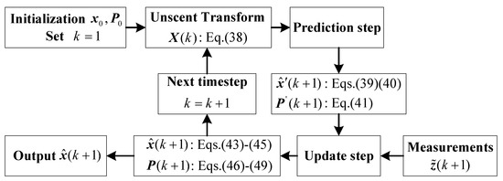
Figure 3.
The flowchart of the estimator after the collision.
4. Observability Analysis
This Section investigates the observability of the estimation model contained the estimator and the estimator . In this paper, estimator is the core of estimating the complete inertial parameters of the object, as well as estimating the attitude and the relative position. Estimator is utilized to filter the measurements of the Euler angles and the relative position of the object. So the estimator is proved to be observable in estimating the motion state which consists of the Euler angles, the angular velocity, the relative position, and the relative velocity of the space object. The estimator is proved to be observable in estimating the motion state and the six inertial parameters. At first, a theorem in references [30,31], which discusses the observability of nonlinear systems, is presented.
Theorem 1.
The following form is used to model the behavior of physical, biological, or social systems,
where is the state vector, is the vector of observed system outputs, and is the vector of control inputs. The Lie derivative of with respect to at is:
where is the partial derivative of with respect to . Let be the observability matrix for the nonlinear system, whose rows are formed from the gradients of the Lie derivatives of . The system is locally weakly observable at if has full column rank at . We say that the system satisfies the observability rank condition at .
According to Theorem 1, the nonlinear system satisfying the observability rank condition is locally weakly observable at . and are introduced to express the observability matrix of estimator and estimator :
Each column in the observability matrix and represents the partial derivative of each parameter of the state vector : 1th–3th columns are the partial derivative of , 4th–6th columns are the partial derivative of , 7th–9th columns are the partial derivative of , 10th–12th columns are the partial derivative of , and 13th–18th columns are the partial derivative of . In the following, the observability of the designed estimators is proved.
4.1. The Observability of Estimator after the Collision
Note that the dimension of the state vector of the estimator is 18. A sufficient condition of the estimator to be observable is that the observability matrix is full-ranked as:
To simplify the expressions of formulas, C, I, , B, and are introduced to substitute , , , , and in Equation (56) in this subsection. Then Equation (56) is rewritten as:
Taking partial derivatives of , , and with respect to , yields:
where is a 3 × 3 identity matrix. is a m × n all-zero matrix. The matrixes , , and represent the partial derivatives of the observation equation to the Euler angles, the angular velocity and the inertial parameters, respectively. The expressions of , , and are given by:
where , , and in Equation (61) represent the transformation matrix corresponding to each rotation of the Euler angles , respectively. The expressions of , , and are given by:
The expressions of and in Equation (63) are defined as:
where , .
The Lie differentiation of with respect to the function is defined by:
where , , and represent the Lie differentiation of , , and with respect to , respectively. The expressions of , , and are presented as:
Then the partial derivative of with respect to the state vector is calculated as:
where the symbol “⊛” represents the matrix component which will not be utilized in proving the observability of the system. – are calculated by:
In Equations (73) and (75), and are not simplified. This is because and contain no inertial parameters. The partial derivative of the terms contained with respect to the inertial parameters are zeros. and in Equation (77) are calculated by:
where represents the i-th row in . in Equation (79) is defined as:
The Lie differentiation of with respect to the function is defined by:
where represents the Lie differentiation of with respect to . The expression of is given by:
Then the partial derivative of with respect to is obtained:
where is the partial derivative of with respect to . is calculated by:
A matrix is introduced to represent a submatrix of the observability matrix :
Note that is composed of the beginning 21 rows of the observability matrix . If is proved, then Equation (53) is proved to be true. In other words, is a sufficient condition for the estimator to be observable. The rank of the identity matrix is 3. For , the rank of is 3. A matrix is introduced:
The rank of is solved by programming in MATLAB. The program is shown in Figure A1. According to the programming results, the rank of is 5 when , and the rank of is 6 when . It means that if the angular velocity of the object is changed by the ball after the collision, the condition expressed as is valid. As a result, the rank of is 6. As , and are column full rank matrix, the rank of is calculated by:
In other words, as long as the angular velocity of the object is affected by the collision between the ball, the rank of the observability matrix is equal to 18. The nonlinear estimator in Equation (37) is observable under the circumstance after the collision between the impact ball and the object.
4.2. The Observability of Estimator before the Collision
In this subsection, the observability of the estimator is proved. Note that estimator is utilized to filter the Euler angles, the angular velocity, the relative position, and the relative velocity. A sufficient condition of the estimator to be observable is that the observability matrix is full-ranked as:
A matrix is introduced to represent the beginning 12 rows of matrix . If is proved, then Equation (88) is proved to be true. Note that is the beginning 12 columns in the beginning 12 rows of matrix . According to Equation (87), the rank of is calculated by:
As a result, estimator is observable in estimating the Euler angles, the angular velocity, the relative position and the relative velocity of the object.
This section proves the observability of the estimation model. Estimator is proved to be observable in estimating the motion state of the defunct object. Estimator is proved to be observable in estimating the motion state and the inertial parameters of the object when the inertia tensor of the defunct object is non-diagonal. Estimator is unobservable for the complete six inertial parameters. When the inertia tensor is diagonal, the inertial parameters only contains the moment of inertial parameters: . In this time, estimator is effective in estimating the three principal axes of the inertial parameters.
5. Numerical Simulations
This section presents numerical simulation examples to demonstrate the performance of the estimation model. The estimation model is composed of two estimators: estimator works when and estimator works when . When , the space object performs an undisturbed attitude motion. At the epoch , the impact ball collides with the object. When , the ball rebounds and crashes into the atmosphere finally. Due to the collision, extra information is introduced into the problem. As a result, the inertia tensor of the object becomes observable, as proved in Section 4. The initial conditions and simulation parameters of the impact ball and the space object are shown in Table 1. In addition, the initial value of is set as km. The initial value of is set as km. The sampling frequency of the measurement system is set as 10 Hz. The initial time is set as s. The ball is ejected from the tracking spacecraft at . In the simulations, is chosen as 200 s. The ball hits the defunct object and adheres to the object at , where . The value of is calculated from the initial parameters, which results in s.

Table 1.
Initial conditions and parameters of the impact ball and the object.
The errors of the estimations of the state variables are defined as:
where represents the estimation errors of the Euler angles, represents the estimation error of the angular velocity, represents the estimation errors of the relative position, represents the estimation error of the relative velocity, and represents the relative errors of the estimations of the inertial parameters. As shown in Equations (90) and (91), the absolute errors are utilized to describe the errors of the Euler angles and the angular velocity to avoid zero-crossing issues, while the relative errors are utilized to describe the errors of the inertial parameters as shown in Equation (92).
5.1. Estimation Results
As introduced in Section 3, the estimation model proposed in this paper contains two estimators: estimator before the collision and estimator after the collision. This subsection presents the simulation results of the estimation model and analyzes the effectiveness of the estimation model. In the simulation, the measured Euler angles are set as the sum of the true values and zero-mean Gaussian white noise signals with the standard deviation of °. The measured relative position is set as the sum of the true value and zero-mean Gaussian white noise with the standard deviation of m. The algorithm is initialized as follows. The initial values of the Euler angles are set as the measured values of the measurement system, the initial value of angular velocity is set as °/s, the initial value of relative position is set as the measured value obtained from the measurement system, the initial value of relative velocity is set as m/s, and the initial values of the inertial parameters are set as kgm2/s.
Figure 4 shows the true values of the object’s states. Figure 4a,b represent the true values of the Euler angles and the relative position of the object. Figure 4c shows that the angular momentum of the object exerts a change when the collision happens at s. The amount of the change of the object is equal to the change of the angular momentum of the ball after the collision.
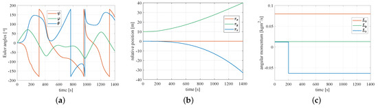
Figure 4.
The true values of the Euler angles, the relative position, and the angular momentum of the defunct space object: (a) true values of the Euler angles; (b) true value of the relative position; (c) true value of the angular momentum.
5.1.1. Before the Collision
This section shows the simulation results of the estimator before the collision. In this phase, the measurements of the Euler angles and the relative position of the object are known.
Figure 5 shows the simulation results of the Euler angles, the relative position, and the inertial parameters of the object. As shown in Figure 5a, the range of the Euler angles is limited to . Figure 5b shows that the errors of the estimated Euler angles are significantly declined within 10 s. At s, is less than °. Figure 5c shows that the estimated errors of the relative position declines from m to m within 20 s. Figure 5d shows that the average value of is less than m when s. However, the estimator has poor performance in estimating the inertial parameters. The dotted lines and the solid lines indicate the true values and the estimations of the inertial parameters in Figure 5e,f. As shown in Figure 5e,f, the relative errors of the estimations of are more than when s. The curves of the estimations of the inertial parameters are divergent in the simulation time. This result demonstrates that the non-diagonal inertia tensor of a defunct object is not observable if only the measured value of the attitude is provided.
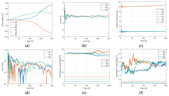
Figure 5.
The estimations of the state variables of the object before the collision: (a) Euler angles estimations; (b) errors of the Euler angles estimations; (c) relative position estimations; (d) errors of the relative position estimations; (e) the moment of inertia estimations; (f) the product of inertia estimations.
5.1.2. After the Collision
This subsection presents the simulation results of the estimator expressed in Equation (37) when . The initial value of the state vector in the estimator is set as the estimation of the state vector of the estimator when . In the numerical simulations in this section, the error of given in Equation (32) is set as 5 percent of the true value of . The estimation results of state parameters are shown in Figure 6, Figure 7 and Figure 8.
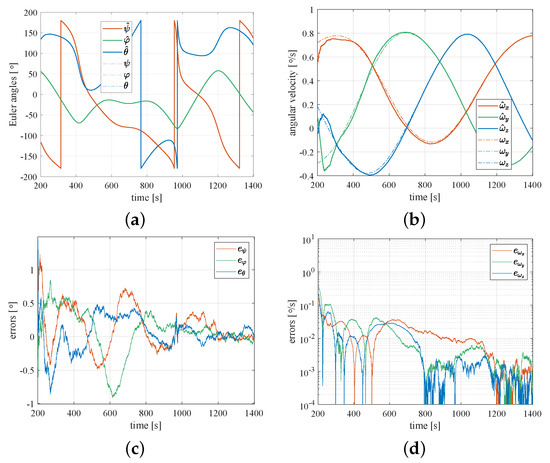
Figure 6.
The estimations of the attitude of the object after the collision: (a) estimations of the Euler angles; (b) estimations of the angular velocity components; (c) errors of the Euler angle estimations; (d) error of the angular velocity estimation.
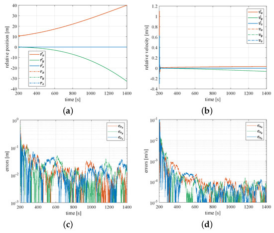
Figure 7.
The estimations of the position state of the object after the collision: (a) estimation of the relative position; (b) estimation of the relative velocity; (c) error of the relative position estimation; (d) error of the relative velocity estimation.
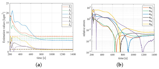
Figure 8.
The estimations of the inertial parameters of the object after the collision: (a) errors of the estimations of the moment of inertia; (b) errors of the estimations of the product of inertia.
Figure 6 shows the estimation results of the Euler angles and the angular velocity after the collision. Figure 6a shows the estimations of the Euler angles. The solid lines and the dotted lines represent the estimations and the true values of the Euler angles, respectively. As shown in Figure 6b, the estimation of the angular velocity has slight fluctuations in the beginning 200 s. It can be seen from Figure 6c,d that the estimations of the Euler angles converge within 100 s. Note that in the simulations the standard deviation of the errors of the measured Euler angles is set to be °. When , the errors of the estimated Euler angles converge to the region , and the error of the angular velocity converges to °/s.
Figure 7 shows the estimation results of the relative position and the relative velocity after the collision. As shown in Figure 7a,b, the initial error of the the relative position is around m, and the initial error of the relative velocity is more than m/s. The estimations of the relative position and the relative velocity converge rapidly within 20 s. Figure 7c,d show the estimation errors of the relative position and the relative velocity. It can be seen from these figures that the relative position converges to m within 100 s. When s, the average of the errors of the relative position estimations is less than m. The average of the errors of the relative velocity estimations is less than m/s. This shows that the estimator is effective in filtering the position and the velocity of the object.
Figure 8a shows the estimations of the inertial parameters of the object. It can be seen that the estimations of the inertial parameters stabilize within 600 s. Figure 8b corresponds to the errors of the estimations of the inertial parameters. The relative errors of the inertial parameters are reduced from to within 800 s. When s, the estimations of the inertial parameters tend to be stable. When s, the average of the errors of the inertial parameters estimations is within . This result demonstrates that the estimator is effective in estimating the complete inertial parameters of the object.
5.2. The Influence of Initial Values of Inertial Parameters
The last subsection presents the simulation results of the estimation model under normal circumstances. This subsection analyzes the influence of the initial values of the inertial parameters on the estimations of the estimator . In the above simulations, the initial inertial parameters are set as kgm2/s. According to Table 1, the true values of the inertial parameters are kgm2/s. The average of the relative errors of the initial inertial parameters is around . In this subsection, the initial inertial parameters are set as kgm2/s. At this time, the relative error of the initial inertial parameters is more than 600%. The total simulation time is set as 2000 s.
Figure 9 shows the errors of the estimations after the collision with the large initial error of . Figure 9a,b show the errors of the Euler angles and the angular velocity estimations of the object. As shown in Figure 9a, the errors of the Euler angles estimations decline from 2° to 0.2° within 1000 s. When s, the estimation errors converge to the region . When s, is around 0.12°. Figure 9b shows that converges to the region /s when s. Figure 9c,d show that the errors of the relative position and the relative velocity estimations decline quickly and converge within 500 s. Figure 9e,f are the errors of the inertial parameters estimations of the object. As shown in Figure 9e,f, the relative errors of the estimations of the inertial parameters decline quickly. Within the simulation time of 1000 s, the curves tend to be converged. The average of the relative error of the inertial parameters is less than when s. The estimation errors of the state variables are tabulated in Table 2. It can be seen from the second line of Table 2 that the estimation model is effective in estimating the state vector of the object when the average of errors of the initial inertial parameters is . The estimation errors of the motion states are basically unchanged compared with the estimations with lower errors of the initial inertial parameters shown in Figure 6 and Figure 7. This demonstrates that the estimation model performs robustly in estimating the motion state and the inertial parameters of the defunct space object.
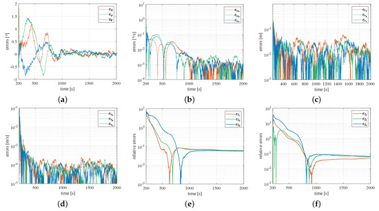
Figure 9.
The errors of the estimations after the collision with large errors of initial inertial parameters: (a) errors of the Euler angle estimations; (b) errors of the angular velocity estimations; (c) errors of the relative position estimations; (d) errors of the relative velocity estimations; (e) errors of the moment of inertia estimations; (f) errors of the product of inertia estimations.
Table 2.
Estimation errors of the state variables when t = 2000 s.
5.3. The Influence of Relative Distance
This subsection analyzes the influence of the relative distance on the estimations of the state variables. In the above simulations, the relative distance is set as 10 m. The measurement error of the relative distance is in proportion to the true value of the relative distance. It means that the larger the distance, the larger the measurement errors of the state variables. It can be seen from Equation (32) that, in the estimation model proposed in this paper, the measurement error of the relative distance is reflected in the error of the angular momentum of . When the relative distance is set as 10 m, the relative error of is assumed as . In this section, the farer relative distance between the object and the tracking spacecraft is considered. The relative distance is set as 100 m. Correspondingly, the relative error of is assumed as .
Figure 10 shows the errors of the state estimations when the relative distance is 100 m. Figure 10a,b are the errors of the Euler angles and the angular velocity estimations of the object. As shown in Figure 10a, the errors of the estimated Euler angles gradually decline within 200 s. is around when s. As shown in Figure 10b, is less than /s when s. Figure 10c,d are the errors of the relative position and the relative velocity estimations. declines from 1 m to m and declines from m/s to m/s within 1000 s. This demonstrates that the estimator after the collision is effective in estimating the motion states when the relative distance between the tracking spacecraft and the object is somewhat large. Compared with the estimations shown in Figure 6 and Figure 7, the errors of the motion state are little larger. However, the relative distance has a slight influence on the estimations of the inertial parameters. Figure 10e,f are the errors of the inertial parameters estimations of the object. As shown in Figure 10e,f, the relative errors of the initial estimations of are more than when s. The estimations of the inertial parameters converge to the region within 1000 s. When s, is less than . The estimation errors of the state variables are tabulated in Table 2. It can be seen from the third line of Table 2 that the estimation model is effective in estimating the state vector when is .
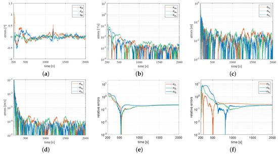
Figure 10.
The errors of the estimations after the collision at large distance: (a) errors of the Euler angle estimations; (b) errors of the angular velocity estimations; (c) errors of the relative position estimations; (d) errors of the relative velocity estimations; (e) errors of the moment of inertia estimations; (f) errors of the product of inertia estimations.
To further analyze the influence of the relative distance on the estimation model, the relative distance between the tracking spacecraft and the object is considered when m. Correspondingly, the error of the angular momentum measurement is set as: . In this section, only the errors of the attitude and the inertial parameters estimations are considered. In order to show the results conveniently, the root mean square (RMS) of the state variables are defined. Different from presented in Equation (90), is defined as the relative RMS of the average values of in the last N estimations of the Euler angles in the simulation time. Similarly, the statistical RMS error of the angular velocity is defined as . The statistical RMS error of the inertial parameters is defined as . , , and are calculated by:
where represents the i-th estimation values among the N estimations of the state variables. In the simulations, N is chosen as 100.
Figure 11 is the statistic results of the RMS relative errors of the states with different relative distance. As shown in Figure 11, and increase slowly with the increase of . Compared with the true values of the Euler angles and the angular velocity, the relative RMS error of the Euler angles is less than and the relative RMS error of the angular velocity is less than . The relative RMS error of the inertial parameters is when the relative distance is 10 m, while is up to when is 100 m. This result demonstrates that the inertial parameters are more sensitive to the relative distance than the attitude and the position.
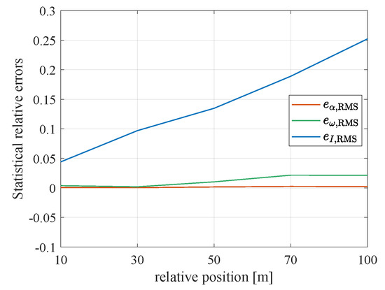
Figure 11.
The statistical RMS relative errors of the attitude and the inertial parameters of the object under different relative distance .
6. Conclusions
This paper proposes a momentum excitation approach which enables the observation of the inertia tensor of a defunct space object with six independent variables. Based on this idea, an impact-rebound based estimation model composed of two estimators is developed. Before the collision happens, the first estimator is engaged to provide a robust estimation of the attitude and the position of the object, while the accurate values of the inertial parameters cannot be obtained. After the collision happens, the second estimator is activated to estimate the attitude, the position and the inertial parameters of the object. The observability of the two estimators is proved theoretically. Numerical simulations illustrate the effectiveness of the parameter estimation model. In addition, the simulations also show that the inertial parameters are more sensitive to the relative distance than the attitude and the position. The estimation model is robust in estimating the state vector under the condition of large initial errors and large relative distance.
Author Contributions
Conceptualization, B.X. and S.W.; methodology, B.X. and S.W.; software, B.X.; validation, S.W.; formal analysis, B.X.; investigation, B.X.; resources, B.X. and S.W.; data curation, S.W.; writing—original draft preparation, B.X.; writing—review and editing, S.W., L.Z. (Liping Zhao) and L.Z. (Long Zhang); visualization, B.X.; supervision, L.Z. (Liping Zhao) and S.W. All authors have read and agreed to the published version of the manuscript.
Funding
This research was funded by Strategic Priority Research Program of the Chinese Academy of Sciences of grant No. XDA30010500, and the Lab funding of the Key Laboratory of Space Utilization of grant No. CXJJ-22S021, and the National Natural Science Foundation of China of grant No. 61903354.
Data Availability Statement
Data available on request from the authors.
Conflicts of Interest
The authors declare no conflict of interest.
Appendix A. The Program of Verifying the Observability of the Estimation Model

Figure A1.
Matlab code calculating the rank of N.
References
- Dubowsky, S.; Papadopoulos, E. The kinematics, dynamics, and control of free-flying and free-floating space robotic systems. IEEE Trans. Robot. Autom. 1993, 9, 531–543. [Google Scholar] [CrossRef]
- Zhu, L.; Wang, S. Rotating Object Specific Tracking Based on Orbit-Attitude Coordinated Adaptive Control. J. Guid. Control Dyn. 2021, 44, 266–282. [Google Scholar] [CrossRef]
- Zhang, S.; Wang, S. Two-Craft Lorentz Force Formation Dynamics and Control. In Proceedings of the IEEE Chinese Guidance, Navigation and Control Conference, Nanjing, China, 12–14 August 2016. [Google Scholar] [CrossRef]
- Philip, N.; Ananthasayanam, M. Relative position and attitude estimation and control schemes for the final phase of an autonomous docking mission of spacecraft. Acta Astronaut. 2003, 52, 511–522. [Google Scholar] [CrossRef]
- Lichter, M.D.; Dubowsky, S. State, shape, and parameter estimation of space objects from range images. In Proceedings of the IEEE International Conference on Robotics and Automation, New Orleans, LA, USA, 26 April–1 May 2004. [Google Scholar] [CrossRef]
- Wilson, E.; Sutter, D.W.; Mah, R.W. MCRLS for On-line Spacecraft Mass-and Thruster-Property Identification. In Proceeding of the IASTED International Conference on Intelligent Systems and Control, Honolulu, HI, USA, 1–6 August 2004. [Google Scholar]
- Wilson, E.; Sutter, D.W.; Mah, R.W. Motion-Based Mass and Thruster-Property Identification for Thruster-Controlled Spacecraft. In Proceedings of the AIAA Infotech @Aerospace Conference, Arlington, VA, USA, 26–29 September 2005. [Google Scholar] [CrossRef]
- Sheinfeld, D.; Rock, S. Rigid Body Inertia Estimation with Applications to the Capture of a Tumbling Satellite. In Proceedings of the 19th AAS/AIAA Spaceflight Mechanics Meeting, Savannah, GA, USA, 8–12 February 2009. [Google Scholar]
- Benninghoff, H.; Boge, T. Rendezvous Involving a Non-Cooperative, Tumbling Target-Estimation of Moments of Inertia and Center of Mass of an Unknown Target. In Proceedings of the International Symposium on Space Flight Dynamics, Munich, Germany, 19–23 October 2015. [Google Scholar]
- Pesce, V.; Lavagna, M.; Bevilacqua, R. Stereovision-based pose and inertia estimation of unknown and uncooperative space objects. Adv. Space Res. 2017, 59, 236–251. [Google Scholar] [CrossRef]
- Hou, X.; Ma, C.; Wang, Z.; Yuan, J. Adaptive pose and inertial parameters estimation of free-floating tumbling space objects using dual vector quaternions. Adv. Mech. Eng. 2017, 9, 1–17. [Google Scholar] [CrossRef]
- Yuan, J.; Hou, X.; Sun, C.; Cheng, Y. Fault-tolerant pose and inertial parameters estimation of an uncooperative spacecraft based on dual vector quaternions. J. Aerosp. Eng. 2018, 233, 1250–1269. [Google Scholar] [CrossRef]
- Nocerino, A.; Opromolla, R.; Fasano, G.; Grassi, M. LIDAR-based multi-step approach for relative state and inertia parameters determination of an uncooperative target. Acta Astronaut. 2021, 181, 662–678. [Google Scholar] [CrossRef]
- Nocerino, A.; Opromolla, R.; Fasano, G.; Grassi, M. Experimental validation of inertia parameters and attitude estimation of uncooperative space targets using solid state LIDAR. In Proceedings of the 73rd International Astronautical Congress, Paris, France, 18–22 September 2022. [Google Scholar]
- Hillenbrand, U.; Lampariello, R. Motion and Parameter Estimation of a Free-Floating Space Object from Range Data for Motion Prediction. In Proceedings of the International Symposium on Artificial Intelligence, Robotics and Automation in Space, Munich, Germany, 5–8 September 2005. [Google Scholar]
- Zhou, B.; Cai, G.; Liu, Y.; Liu, P. Motion prediction of a non-cooperative space target. Adv. Space Res. 2018, 61, 207–222. [Google Scholar] [CrossRef]
- Murotsu, Y.; Tsujio, S.; Senda, K.; Mitsuya, A. System identification and resolved acceleration control of space robots by using experimental system. In Proceedings of the IEEE/RSJ International Workshop on Intelligent Robots and Systems, Osaka, Japan, 3–5 November 1991. [Google Scholar] [CrossRef]
- Murotsu, Y.; Senda, K.; Ozaki, M.; Tsujio, S. Parameter identification of unknown object handled by free-flying space robot. J. Guid. Control Dyn. 1994, 17, 488–494. [Google Scholar] [CrossRef]
- Yoshida, K.; Abiko, S. Inertia parameter identification for a free-flying space robot. In Proceedings of the AIAA Guidance, Navigation, and Control Conference, Monterey, CA, USA, 5–8 August 2002. [Google Scholar] [CrossRef]
- Nguyenhuynh, T.C.; Sharf, I. Adaptive Reactionless Motion and Parameter Identification in Postcapture of Space Debris. J. Guid. Control Dyn. 2013, 36, 404–414. [Google Scholar] [CrossRef]
- Felicetti, L.; Sabatini, M.; Pisculli, A.; Gasbarri, P.; Palmerini, G.B. Adaptive Thrust Vector Control during On-Orbit Servicing. In Proceedings of the AIAA SPACE 2014 Conference and Exposition, San Diego, CA, USA, 4–7 August 2014. [Google Scholar] [CrossRef]
- Meng, Q.; Liang, J.; Ma, O. Identification of all the inertial parameters of a non-cooperative object in orbit. Aerosp. Sci. Technol. 2019, 91, 571–582. [Google Scholar] [CrossRef]
- Meng, Q.; Zhao, C.; Ji, H.; Liang, J. Identify the Full Inertial Parameters of a Non-cooperative Target with Eddy Current Detumbling. Adv. Space Res. 2020, 66, 1792–1802. [Google Scholar] [CrossRef]
- Liu, X.; Zhang, X.; Chen, P.; Cai, G. Inertia Parameter Identification for an Unknown Satellite in Precapture Scenario. Int. J. Aerosp. Eng. 2020, 2020, 7521434. [Google Scholar] [CrossRef]
- Xu, B.; Wang, S. Vision-Based Moment of Inertia Estimation of Non-Cooperative Space Object. In Proceedings of the International Symposium on Computational Intelligence and Design, Hangzhou, China, 9–10 December 2017. [Google Scholar] [CrossRef]
- Xu, B.; Wang, S.; Zhao, L. Mechanism of collision and adhesion between adhesive impact ball and spacecraft. In Proceedings of the 3rd International Conference on Applied Mechanics and Mechanical Engineering, Xi’an, China, 23–25 December 2022. [Google Scholar]
- Schaub, H.; Junkins, J. Analytical Mechanics of Space Systems, 4th ed.; American Institute of Aeronautics and Astronautics: Reston, VA, USA, 2018. [Google Scholar] [CrossRef]
- Fisher, J.; Vadali, S.R. Gyroless Attitude Control of Multi-Body Satellites Using an Unscented Kalman Filter. J. Guid. Control Dyn. 2008, 31, 245–251. [Google Scholar] [CrossRef]
- Soken, H.E.; Cilden, D.; Hajiyev, C. Attitude Estimation for Nanosatellites Using Singular Value Decomposition and Unscented Kalman Filter. In Proceedings of the International Symposium on Space Technology and Science, Hyogo, Japan, 4 July 2015. [Google Scholar]
- Hermann, R.; Krener, A. Nonlinear controllability and observability. IEEE Trans. Autom. Control 1977, 22, 728–740. [Google Scholar] [CrossRef]
- Kelly, J.; Sukhatme, G.S. Visual-Inertial Sensor Fusion: Localization, Mapping and Sensor-to-Sensor Self-calibration. Int. J. Robot. Res. 2010, 30, 56–79. [Google Scholar] [CrossRef]
Disclaimer/Publisher’s Note: The statements, opinions and data contained in all publications are solely those of the individual author(s) and contributor(s) and not of MDPI and/or the editor(s). MDPI and/or the editor(s) disclaim responsibility for any injury to people or property resulting from any ideas, methods, instructions or products referred to in the content. |
© 2023 by the authors. Licensee MDPI, Basel, Switzerland. This article is an open access article distributed under the terms and conditions of the Creative Commons Attribution (CC BY) license (https://creativecommons.org/licenses/by/4.0/).