ProgNet: A Transferable Deep Network for Aircraft Engine Damage Propagation Prognosis under Real Flight Conditions

Abstract

Machine learning prognosis for condition monitoring of safety-critical systems, such as aircraft engines, continually faces challenges of data unavailability, complexity, and drift. Consequently, this paper overcomes these challenges by introducing adaptive deep transfer learning methodologies, strengthened with robust feature engineering. Initially, data engineering encompassing: (i) principal component analysis (PCA) dimensionality reduction; (ii) feature selection using correlation analysis; (iii) denoising with empirical Bayesian Cauchy prior wavelets; and (iv) feature scaling is used to obtain the required learning representations. Next, an adaptive deep learning model, namely ProgNet, is trained on a source domain with sufficient degradation trajectories generated from PrognosEase, a run-to-fail data generator for health deterioration analysis. Then, ProgNet is transferred to the target domain of obtained degradation features for fine-tuning. The primary goal is to achieve a higher-level generalization while reducing algorithmic complexity, making experiments reproducible on available commercial computers with quad-core microprocessors. ProgNet is tested on the popular New Commercial Modular Aero-Propulsion System Simulation (N-CMAPSS) dataset describing real flight scenarios. To the extent we can report, this is the first time that all N-CMAPSS subsets have been fully screened in such an experiment. ProgNet evaluations with numerous metrics, including the well-known CMAPSS scoring function, demonstrate promising performance levels, reaching 234.61 for the entire test set. This is approximately four times better than the results obtained with the compared conventional deep learning models.

1. Introduction

Safety-critical systems, such as aircraft engines, require continuous preventive maintenance, planned through accurate decision-making. Indeed, maintenance tasks are very crucial as they are the main reason potential reputational and financial loss incidents are avoided, as well as what would probably be catastrophic loss of life [1]. For the maintenance program of aircraft engine components, real-time estimation of the remaining useful life (RUL), which is the time between the moment of loss and the complete failure of the system, is an absolute necessity [2,3,4]. Besides, one must have access to an accurate modeling process dealing with dynamic changes under harsh working conditions, whether through data-driven or physical modeling [5]. Due to the complexity, difficulty, and problems in generalizing mathematical interpretations of physical phenomena occurring in aircraft engines, data-driven methods has become more dominant in recent research. As a result, this paper introduces a domain adaptation data-driven method for RUL prediction of aircraft engines under real flight conditions. Accordingly, this section mainly describes the motivation behind the proposed method, illustrates the main research gap of RUL prediction for aircraft engines, and highlights the proposed solutions to model degradations in aircraft engines.

1.1. Motivation

The complexity, difficulty, and poor generalization of physical modeling have led to machine learning methods dominating in the field, especially with the emergence of advanced sensing technologies [6,7]. RUL model reconstruction for aircraft engines is usually subject to data unavailability, complexity, and drift [2,8]. First, in the context of data unavailability, run-to-failure trajectories are usually collected by simulating non-linear equations related to physical operating principles, but this is only because of the scarcity of failure patterns in such a safety-critical system. In this case, the generated data will by chance suffer from the lack of real-time degradation patterns. Second, these generated data must contain harsh environment readings depicted in the distortion and corruption of sensor measurements, leading to a complex feature space. Finally, the dynamic change of working conditions, due to the physical deterioration of the components of the aircraft and also to the time-varying external conditions, leads to non-linearity and non-stationarity of data (i.e., data drift). Projecting these features onto the model selection flowchart (see Figure 2 and Section 2.2 of [2]), the best choice would be an adaptive deep learning model with generative modeling capabilities to overcome the unavailability, complexity, and dynamism of data.

1.2. Related Works

As mentioned earlier, and since this paper is studying the N-CMAPSS data repository, it is better to ensure that the literature review and research gap analysis also address the contributions made to a particular topic. Therefore, analysis of related works will be very convenient to track recent advances in a specific problem. It is worth mentioning that the collection of papers was carried out by tracking citations of the introductory paper of N-CMAPSS in the Web of Science and Scopus databases and including all contributions published to date [9]. We used the publisher citations tracker on its website (i.e., the HTML version of the paper) and downloaded all papers citing this work. After that, we excluded all papers, except for those dealing with the RUL model reconstruction problem. In total, only four papers dealing with the specific topic of RUL prediction using the N-CMAPSS dataset were found.

For instance, in [10], an uncertainty-aware Gaussian regression process, exposed to complex non-linear deep representations, is used to predict the RUL of aircraft engines. Moreover, complexity is seen as a deep representation problem that could be solved by providing uncertainty estimates of RUL predictions. Therefore, only one N-CMAPSS file among the 8 provided ones is adopted to support the obtained conclusions on the RUL modeling. In [11], a health index prediction model is used to predict engine health state rather than RUL provided with the dataset. This selection is justified by the inability to find real patterns in the simulation data, and the fact health indexes will work better. An anticausal framework with reduced complexity is defined to assess health indexes with a causal driver and Granger causality. Healthy cycles of offline learning are used to generalize online predictions. Similarly, using a single file from the N-CMAPSS dataset, the algorithm shows its capability in reducing the root-mean-squared error (RMSE) by almost 65%, outperforming deep learning methods. The work presented in [12] formulates the near future RUL prediction as a two-level optimization. A long short-term memory (LSTM) network is used as a primary training algorithm due to its sequential training capability. The entire old C-MAPSS dataset and a single N-CMAPSS subset are used for evaluation in cases where results show promising performances. In [13], a hybrid physical model and convolutional neural network (CNN) algorithm are used to approximate sensor run-to-failure readings for a fleet of turbofan engines, assessing RUL under real flight conditions. The designed model shows that it requires less training samples and shows less sensitivity to the lack of patterns compared to purely data-driven approaches.

Table 1. Related works to N-CMAPSS dataset.

Refs	Year	Unavailability	Complexity	Drift
[10]	2021	✗	Using an uncertainty aware deep Gaussian process regression.	✗
[11]	2022	✗	Predicting health indexes with a causal driver and Granger causality.	✗
[12]	2022	✗	Two-level optimization LSTM.	Recursive learning of LSTM allows researchers to address dynamic adaptation towards change in data via forgetting mechanism.
[13]	2022	✗	CNN.	✗
This paper	2022	Cross-modality transfer learning is used to overcome lack of degradation patterns.	LSTM network with adaptive optimization, PCA empirical Bayesian method based on wavelets with a Cauchy prior, and scaling.	Recursive learning of LSTM with adaptive optimization (Adam) allows researchers to address dynamic adaptation towards change in data via forgetting mechanism.

is a summary of contributions of aforementioned works made on the N-CMAPSS dataset in the context of treating RUL challenges. It is noticeable that all these works treat RUL prediction from the perspective of data complexity. In other words, they consider that the non-stationarity and non-linearity of obtained measurements are the main problems facing the training process. This is the reason for building very complex mapping spaces, ranging from deep non-linear abstractions [10,11,13] to deep ensemble learning [12]. In addition, efforts have been made to improve curve fitting by taking into account score functions, RMSE, and uncertainty reductions. These works have achieved excellent results in addressing this aspect of RUL challenges.

1.3. Contributions

Unlike previously discussed works, which mostly dealt with data complexity only, this work aims to achieve greater generalization when predicting RUL for unseen samples. As a result, all data constraints of RUL predictions of aircraft engines (i.e., lack of actual degradation patterns, data complexity, data rapid change, and dynamism) are taken into account. Accordingly, our contributions are listed as follows:

• Targeting data unavailability issues: To solve the problem of lack of degradation patterns, seen due to shortcomings of poor physical modeling generalization, a domain adaptation transfer learning approach is involved in these experiments. The transfer learning approach aims to transfer training parameters across models from a source domain to a target domain for RUL prediction [14]. Source domains include PrognosEase, a data generator for health deterioration prognosis. In the first attempt, the RUL model will be trained to different degradation scenarios with a sufficient number of samples. Then, the trained model will be moved for more fine-tuning to obtain a more accurate RUL prediction.
• Solving a problem of data complexity: The RUL prediction problem is usually a time series analysis under a higher level of data non-stationarity and non-linearity. In this context, LSTM, which is a well-known deep architecture with the ability to map sequential data into a more meaningful space, is considered to correlate between sequential samples. Additionally, well-structured feature engineering of dimensionality reduction, feature selection, denoising, and scaling is used to achieve the meaningful data representations needed for training.
• Rapid change in data dynamism: The aircraft engine RUL prediction also demonstrates a massive and rapid change in data characteristics, resulting from a change in environmental conditions and the physical properties of the system. In this case, LSTM also has the ability to serve adaptive learning through a forgetting mechanism. Moreover, adaptive optimization of learning parameters (Adam) will be more advantageous in online learning to combat the problem of data drift.
• Reducing algorithmic complexity: The proposed feature engineering and transfer learning also help to use fewer non-linear abstractions, with fewer mapping features also, and yet are still able to process meaningful representations with fewer computational costs.
• Precision analysis and uncertainty quantification: To ensure the accuracy of the designed prognostic system, well-known prognostic metrics are adopted in this work. These include scoring functions for early and late prediction penalization, in addition to uncertainty quantification via confidence range assessment at 90%, 95%, and 99%, respectively.

This paper is organized as follows: besides the introductory section, Section 2 is dedicated to the RUL description problem presented in the N-CMAPSS dataset and the following preprocessing steps. Section 3 is devoted to explaining the designed ProgNet and its main training features. Section 4 is set aside for RUL model training and evaluation experiments. Section 5 concludes this paper with prospects.

2. Problem Description and Data Processing

Unlike the original version of the CMAPSS dataset [15], which looks purely like a generation of sensor measurements based on prior assumptions of working flight conditions and failures, the N-CMAPSS is introduced to address more realistic scenarios, using data from real flight conditions as the main material to generate sensor measurements [9]. Many details have been revealed in the introductory publications of the N-CMAPSS dataset, as well as in the original experimental papers of the same dataset team of developers [9,10,13]. However, in this section, we focus on delving into the challenges of RUL in the context of data complexity and showing the advantages of the new system over the legacy CMAPSS data repository.

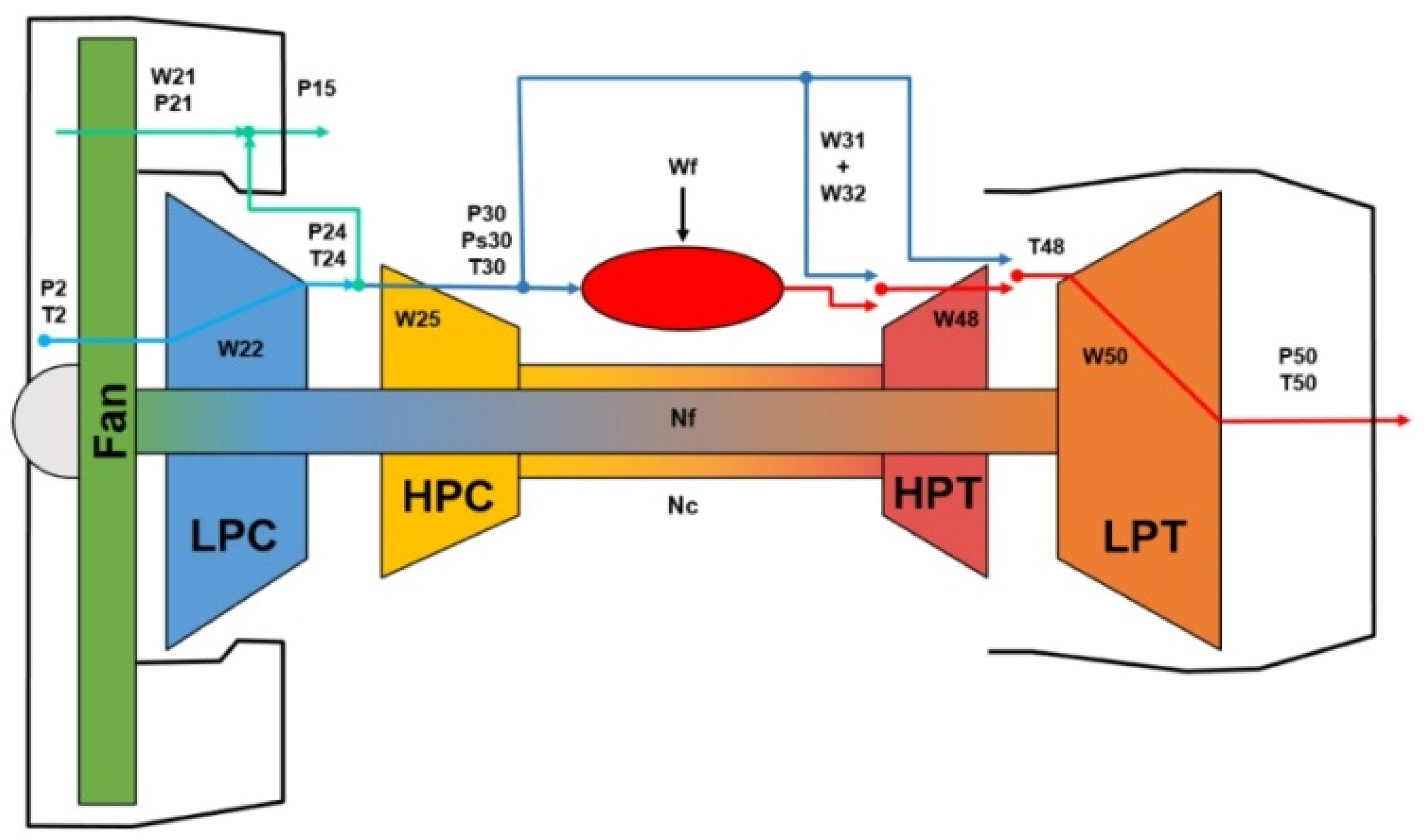
The CMAPSS software contains a high-fidelity dynamic model for simulating a wide range of thrust levels of the tow-spool turbofan engine. Figure 1 gives an excellent overview of the joint physical model and the modeling characteristics. It also gives the detailed positioning of the modeling parameters. When generating the N-CMAPSS dataset, it is assumed that all rotating engine subcomponents, i.e., fan, low-pressure compressor (LPC), high-pressure compressor (HPC), low-pressure turbine (LPT), and high-pressure turbine (HPT), are prone to health deterioration in terms of flow and efficiency. Unlike the original C-MAPSS dataset, five components were studied, instead of two in terms of failure prognosis.

The turbofan assembly can mimic atmospheric operating conditions at altitudes from sea level up to 40,000 feet and Mach numbers from 0 to 0.90. In addition, the simulation model is also capable of varying sea level temperatures from −60 to 103 Fahrenheit. The package also includes a power management system that allows the engine to operate over a wide range of thrust levels, across the full range of flight conditions. For simplicity, the CMAPSS software can be viewed as a non-linear function, $F$, that takes information about operating conditions, $w\left(t\right)$, and health parameters, $\theta \left(t\right)$, to generate sensor measurements$, x_s\left(t\right)$, describing the measured physical properties and the unobserved virtual sensors properties$, x_v\left(t\right)$, measurements. These have nothing to do with automotive health status as explained in (1), where $t$ refers to relative time.

$$\left[x_s\left(t\right), x_v\left(t\right) \right]=F\left(w\left(t\right), \theta \left(t\right)\right)$$

(1)

As mentioned earlier, this section focuses on data behavior in the context of complexity; we paid more attention to studying the recorded $x_s\left(t\right)$ and RUL data necessary for the reconstruction of the machine learning model. Accordingly, this section reveals details about these parameters, while other parameters $\{x_v\left(t\right), F\left(w\left(t\right)\right), \theta \left(t\right)\}$ and other auxiliary data are detailed in [9,10,13]. In this context,

Table 2. Sensors physical properties.

#	Symbol	Description	Unit	#	Symbol	Description	Unit
01	Wf	Fuel flow	pps	08	P15	Total pressure in bypass duct	psia
02	Nf	Physical fan speed	rpm	09	P2	Total pressure at fan inlet	psia
03	Nc	Physical core speed	rpm	10	P21	Total pressure at fan outlet	psia
04	T24	Total temperature at LPC outlet	R	11	P24	Total pressure at LPC outlet	psia
05	T30	Total temperature at HPC outlet	R	12	Ps30	Static pressure at HPC outlet	psia
06	T48	Total temperature at HPT outlet	R	13	P40	Total pressure at burner outlet	psia
07	T50	Total temperature at LPT outlet	R	14	P50	Total pressure at LPT outlet	psia

depicts information regarding obtained sensors measurement used for RUL perdition. At this stage, we think of the generated data as a couple of {$x_v\left(t\right), RUL$}.

Eight datasets from nine turbofan engine fleets have been generated to construct N-CMAPSS measurements, while each dataset is generated to expose important details about specific failure modes for specific life cycles (i.e., units) of the engine. It should be mentioned that data is designed for both diagnosis and prognosis. In this work we paid more attention to the prognosis problem. Therefore, details of the dataset explained in

Table 3. Overview of the N-CMAPSS dataset.

Names	#Unites	Failure Modes	Names	#Unites	Failure Modes
DS01	10	Efficiency of HPT	DS05	10	Efficiency and flow of HPC
DS02	9	Efficiency of HPT, Flow and efficiency of LPT	DS06	10	Efficiency and flow of HPC and LPC
DS03	15	Efficiency of HPT, Flow and efficiency of LPT	DS07	10	Efficiency and flow of LPT
DS04	10	Flow and efficiency of the fan	DS08	54	Efficiency and flow of all components

discuss the main issue of prognosis only.

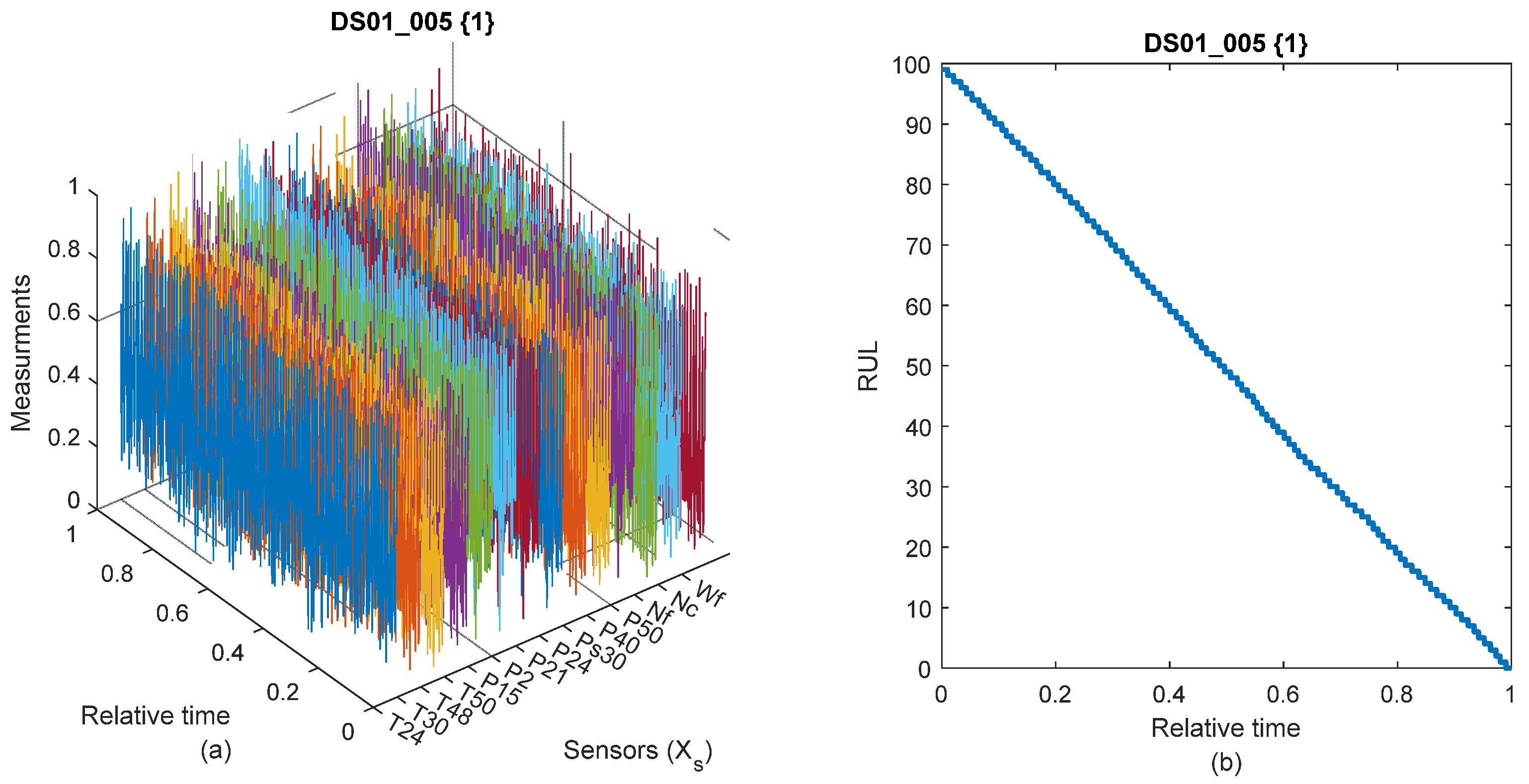
The generated data for the N-CMAPSS dataset are massive (i.e., millions of samples), dynamically and rapidly changing, and measurements are corrupted with a higher level of unknown source noise. Figure 2 displays an example of an entire degradation path from the N-CMAPSS. In this case, the difference between old CMAPSS degradation trajectories (see Figure 1 from [7]) and those of the N-CMAPSS dataset is that the former is able to show a kind of exponential degradation, reflecting the deterioration of engine components. In contrast, it is difficult to observe such a phenomenon in the N-CMAPSS dataset measurements, which is exactly where the data complexity lies.

To improve feature representations for N-CMAPSS to at least delve into these degradation patterns in data, well-structured feature engineering is proposed and tested in this paper. Indeed, feature preprocessing involves denoising, dimensionality reduction, feature selection, and scaling.

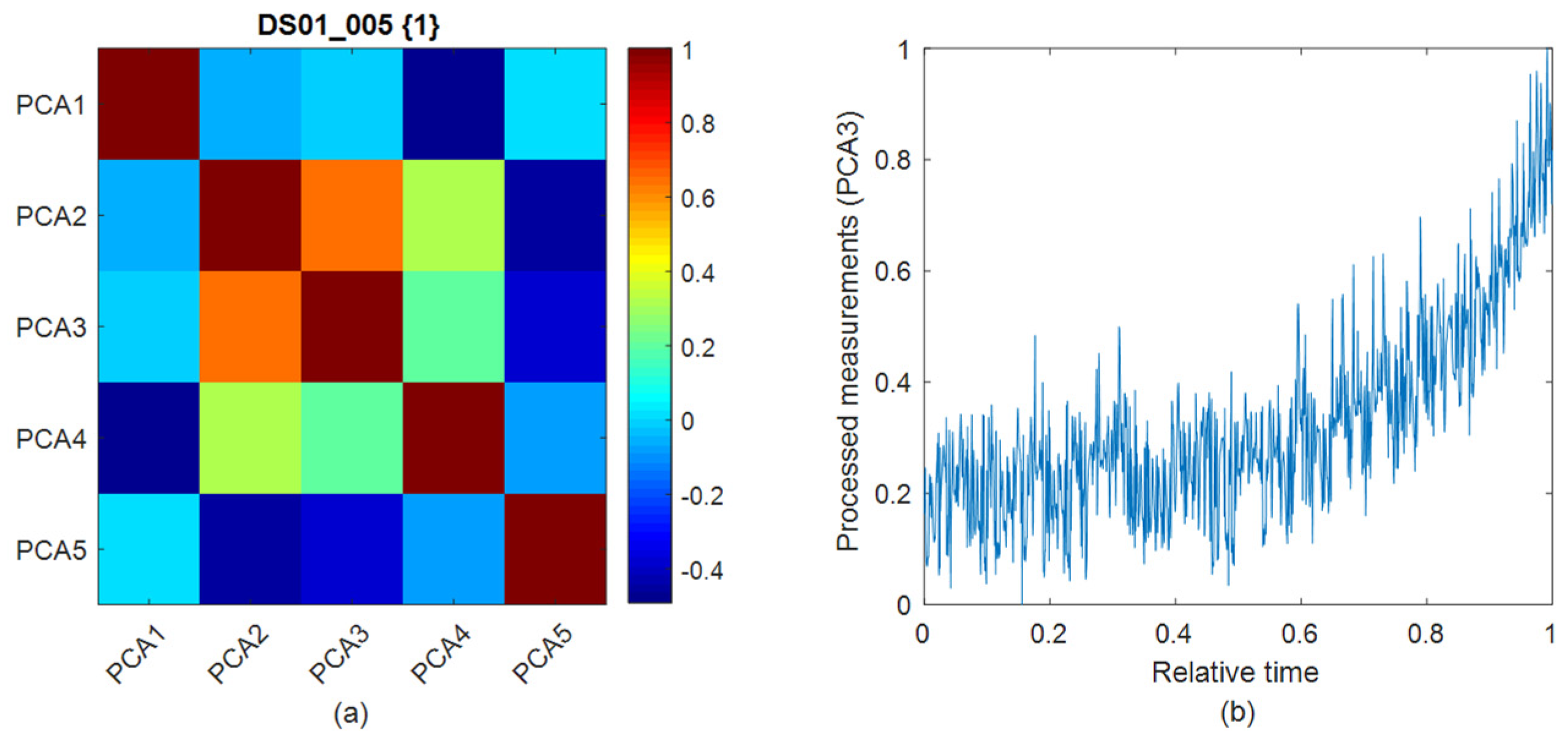
MATLAB R2018b toolkits are used to simplify feature processing. First, a wavelet denoising toolkit, based on the empirical Bayesian wavelet method with a Cauchy prior used with a posterior median threshold rule, is involved to extract robust representations of the obtained features [16]. Second, PCA is used to reduce the feature dimensions from 14 to 5 samples, a change based on the singular value decomposition algorithm. For the selection of PCA components, we used a blackbox model involving a simple permutation test where the explained variance is calculated and compared to the explained variance of the original data. This means that, if a component is relevant, the explained variances are not greater than the original variance. Additionally, a main machine learning test might be more beneficial in determining whether accuracy is similarly maintained at the same original space, even under lossy compression. After that, further feature selection is involved, based on correlation analysis and heatmap visualization, to obtain the final features, ready to be fitted to the training model. Figure 3 deals with the obtained features after scaling with min–max normalization (the heading of the subplot refers to the file name as mentioned in the dataset and unit number). In this case, the third and second components of PCA show a strong correlation, making them excellent candidate features for the training process. However, after some primary testing, we find that the third PCA component shows more accuracy, thus leading to its selection for training. In addition, the data visualization shows a reasonable deterioration of the measurements, reflecting the degradation phenomena of the turbofan engine.

3. Prognosis Scheme

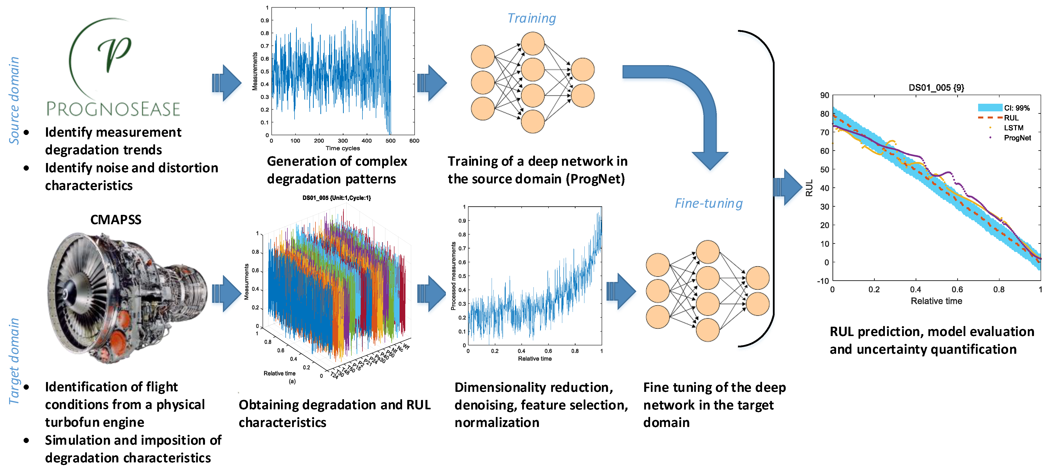
In the proposed transfer learning model, we involve an LSTM network and PrognosEase software for training in the source domain, as addressed in Figure 4 [17].

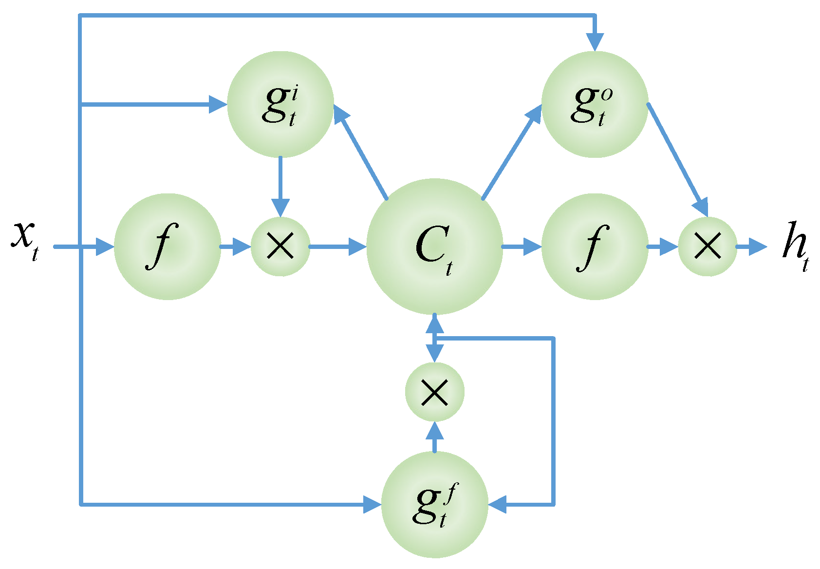
As shown in Figure 5 flowchart, the LSTM network uses the input gate $g_t^i$, output gate $g_t^o$, and a forgetting gate$g_t^f$, as presented in (2), (3), and (4), to control adaptive learning features. The LSTM state is computed using the hidden state $h_t$ and cell state $C_t$ as in (5) to (8) using inputs $x_t$ weights ($w_f$,$w_i$,$w_o$,$w_h$,$w_c$) and biases ($b_f$, $b_i$, $b_o$, $b_h$, $b_c$). The output is calculated as in (8) by involving the output weights, $W_{oh}$, output bias vector, $b_o$, and the activation function, $f$. $f$ is a sigmoid function and $tanh$ is a hyperbolic tangent function.

$$g_t^f=f\left(w_f\left[h_{t-1}+x_t\right]+b_f\right)$$

(2)

$$g_t^i=f\left(w_i\left[h_{t-1}+x_t\right]+b_i\right)$$

(3)

$$g_t^o=f\left(w_o\left[h_{t-1}+x_t\right]+b_o\right)$$

(4)

$$h_t=f\left(w_h\left[h_{t-1}+x_t\right]+b_h\right)$$

(5)

$${\tilde{C}}_t=tanh\left(w_c\left[h_{t-1}+x_t\right]+b_c\right)$$

(6)

$$C_t=g_t^f{C}_{t-1}+g_t^i{\tilde{C}}_{t-1}.$$

(7)

$$O_t=f\left(W_{oh}{h}_t+b_o\right)$$

(8)

PrognosEase is an open source data generator that is used to generate degradation measurements and corresponding RUL functions according to the user’s specified trends. PrognosEase software allows the emulation of real-alike conditions by adding noise and distortion features to measurements. The measurement collection process follows different types of paths, including a linear path, as for batteries [18,19], an exponential path, as for turbofan engines [6,7], and an exponentially grown sinusoidal path, as for bearings and rotating elements [20]. PrognosEase also has the possibility of addressing both cyclic and non-cyclic degradation [21]. These degradation paths can be associated with linear and or exponential RUL degradation trends. These trends are made available by studying a wide range of real applications in the literature. In this paper, a large number of life cycles, including multiple types of measurements associated with linear RUL measurements, are generated to train the ProgNet in the source domain. The goal was to push any noisy distorted representations to an appropriate RUL target, while resisting overfitting through regularization. Therefore, we consider the transfer of learning knowledge from the PrognosEase domain to the N-CMAPSS domain to be very useful for covering the lack of deterioration patterns, seen due to the sharing of the measurement deterioration phenomenon between the two. This is especially the case when N-CMAPSS is misgeneralization software, a situation which occurs when it is built on the physical modeling.

ProgNet is a two-layer LSTM, with twenty neurons per layer and an adaptive optimization capability. Thus, compared to previous introduced deep network architectures [10,11,12,13], in particular compared to CNN [13] and multi-level LSTM [12], the architecture is significantly lightweight. This is the meaning of our fourth contribution to the reduction in algorithmic complexity. Hyperparameters, such as the number of neurons (20), $l_2$ norm-based regularization (0.1), learning rate (0.01), mini-batch sizes (250), and number of epochs (3000), are manually tuned following their use on a trial-and-error basis. This follows the recommendations made in [2] for complex massive data, where evolutionary and swarm intelligence or even grid search will be highly computationally expansive (see Figure 2 from [2]). The purpose of using two LSTM layers is to keep one last layer of fine-tuning of ProgNet in the target domain. The training process of the ProgNet is evaluated using the score function $S$ and RMSE, proposed in [9] for the evaluation of prognosis systems, as showcased in (9) and (10), respectively. Where $\left\{y,\check{y}\right\}$ are the desired and predicted RULs, respectively. $E$ is the prediction error and $\alpha$ is a penalization parameter, defined as $\alpha =\frac{1}{13}$ when $E<0$ and as$\alpha =\frac{1}{10}$ if $E\ge 0$. For ProgNet, $S=2.5667$ and $RMSE=0.1275$ are very satisfactory results obtained during training.

$$RMSE=\frac{1}{N}{\sum }_{i=1}^N\sqrt{\left(E^2\right)}|C \left(y-\check{y}\right)$$

(9)

$$S=\frac{1}{N}{\sum }_{i=1}^N{e}^{\left(\frac{\alpha }{E}\right)}$$

(10)

4. Results and Discussion

For the target domain, the entire dataset is used for fine-tuning the trained ProgNet. The loss function of ProgNet in both domains is set by default to the RMSE function, as previously described in (9). Generally speaking, the global loss function to be minimized is the sum of the losses in both domains. Besides previously mentioned evaluation metrics (i.e., $S$ and$RMSE$), the uncertainty of ProgNet is also quantified at 90%, 95%, and 99% confidence. In this context, Gaussian distributed measurement noise-based confidence interval (CI), as in [22], is calculated to provide insight into the uncertainties of the predictions. Accordingly, formulas (11–12) will be used to determine intervals for each prediction with the help of the total prediction error variance$, {\delta }^2$, prediction variance, ${\delta }_y^2$, and Gaussian noise variance$, {\delta }_g^2$, while $z=\left\{1.65, 1.96, 2.85\right\}$ for 90%, 95%, and 99% confidence, respectively. In this work, we have calculated the ratio of predictions inside the CI over the total number of predictions to estimate the prediction confidence of the proposed approach.

$$CI=y\pm z\sqrt{{\delta }^2}$$

(11)

$${\delta }^2={\delta }_y^2+{\delta }_g^2$$

(12)

Machine learning experiments are carried out using MATLAB R2018b, installed on a quad-core i7 microprocessor laptop with 8 GB of RAM 12 MB of cache memory.

Table 4. Obtained evaluation results.

Algorithm	$\mathit{S}$	$\mathit{R}\mathit{M}\mathit{S}\mathit{E}$	Confidence Level			Important Notes
			90%	95%	99%
[10]	-	7.31	-	-	-	These works considered only a subset of the eight N-CMAPSS subsets.
[11]	-	6.61	-	-	-
[12]	2.188 × 106	6.867	-	-	-
LSTM	878.043	6.01	0.69	0.69	0.69	These works considered the entire N-CMAPSS.
ProgNet	234.61	5.64	0.81	0.79	0.73

summarizes the obtained results of ProgNet, compared to the LSTM network with the same architecture without transfer learning. The results show that ProgNet clearly outperforms the original LSTM with a higher level of performance. Besides, LSTM shows more prediction uncertainties in RUL estimations.

The reason for the high approximation capability of ProgNet is related to the additional information obtained from training on the PrognosEase data, which allows a simpler architecture to be used than those presented in the literature to achieve a higher level of accuracy with lower computational costs. This means that transfer learning helps overcome the problems of lack of damage propagation patterns, resulting from the poor generalization of physics-informed models of the turbofan engine. As a result, the first ProgNet layer (i.e., LSTM layer), which is dedicated to training in the source domain, acts as a generative model, providing more meaningful representations to the N-CMAPSS samples in the target domain. The generated mixture of different measurement types and RUL trends from PrognosEase helps ProgNet to learn deterrent degradation cases and increase knowledge about real-alike samples. This means that the learned representations of the PrognosEase source domain are responsible for pushing the N-CMAPSS patterns to behave appropriately, even if the first feature space is missing meaningful representations.

Comparing the results obtained in works performed so far in the literature on the N-CMAPSS dataset [10,11,12,13], this work obviously achieves better results, although it is the only one investigating the whole dataset under simplest learning rules and algorithmic architecture. It is also noticed that the LSTM network without transfer learning achieved a better performance than that seen in previous works. This is also a proof of the robustness of the designed features engineering. This means that the new feature engineering helps to provide better representations of the raw data features than others provided in the literature.

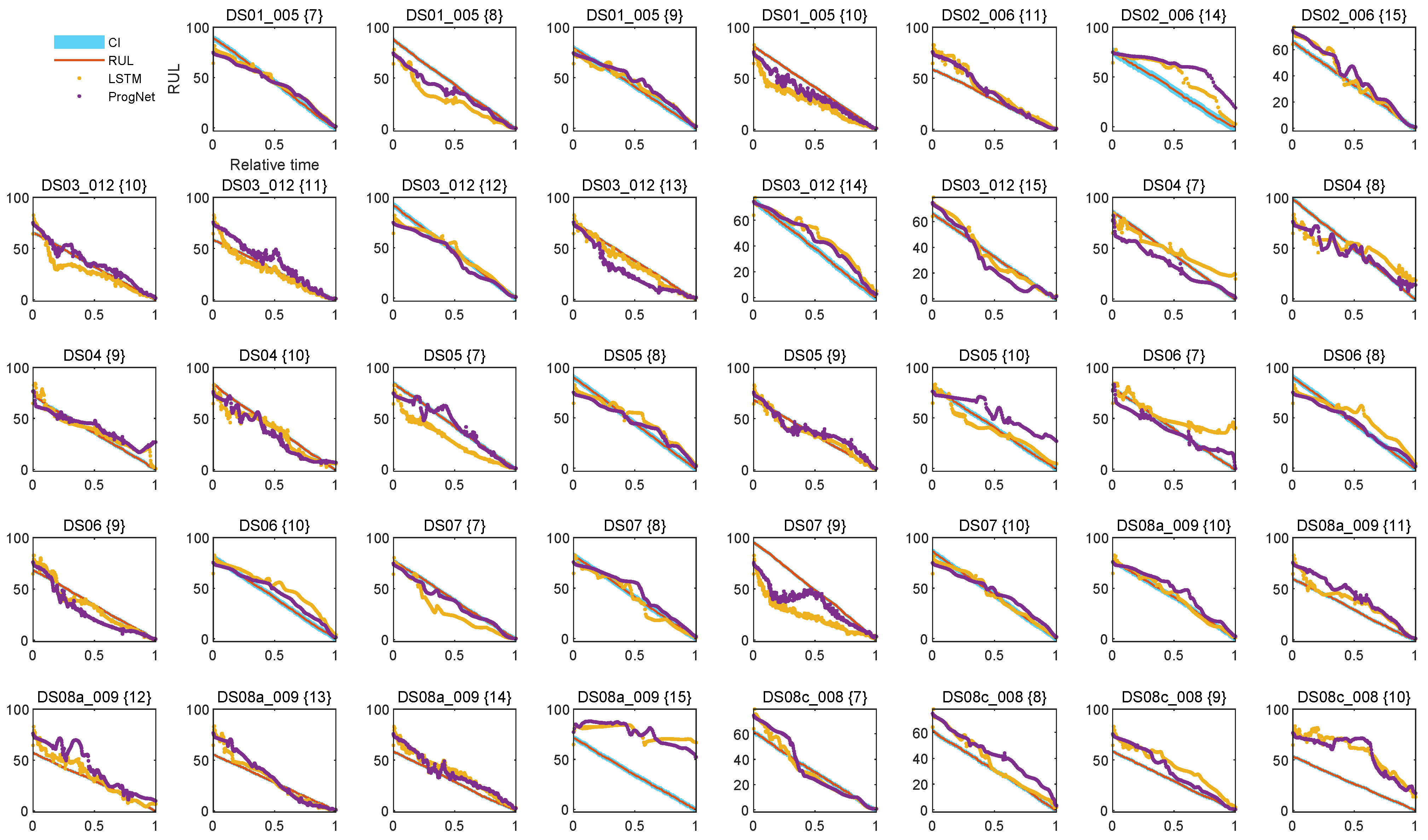
The curve fit of Figure 6 for the entire test set is also strong evidence of the capability of ProgNet, as well as the designed feature engineering process in emulating the degradation trend. Figure 6 depicts curve fits, obtained by LSTM and ProgNet networks, and also showcases the CI range at 99%. The heading in the subplots refers to the file names and the number of testing units. The curve fit is perfectly performed for most of the dataset except for units DS02_006 {14}, DS02 {7}, DS08a_009 {15}, DS08c_008 {10}, DS07 {9}, which suffer from a higher level of fluctuations. These fluctuations are responsible for affecting the accuracy of the entire learning model.

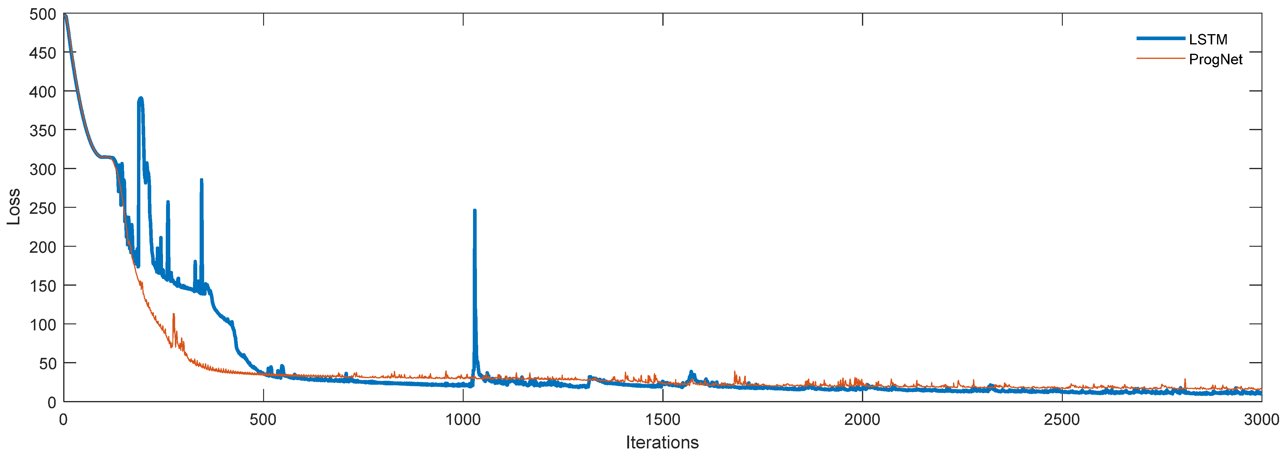
In Figure 7, the loss function behavior of ProgNet with respect to the LSTM network explains the smoothness, rapid convergence, and better stability of the transfer learning process compared to PrognosEase. Seemingly, ProgNet not only contributes to accurate predictions but also makes the model immune to overfitting, and this reason explains the stability within a larger error than the LSTM network in the training phase.

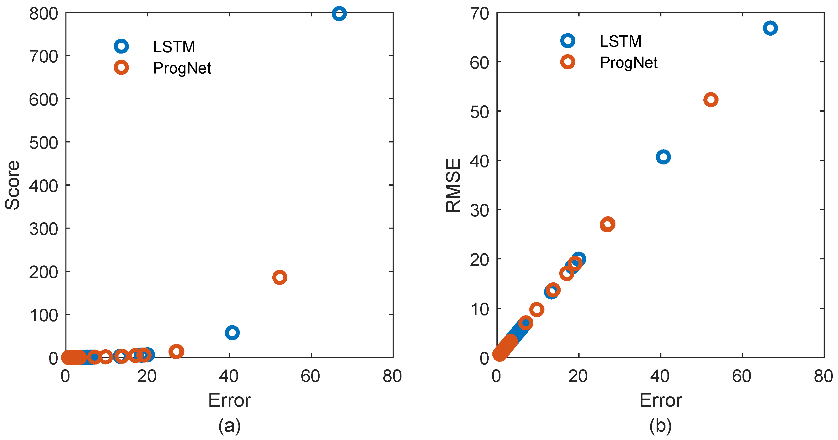
Finally, Figure 8 examines the behavior of the scoring function when testing the model on the N-CMAPSS test samples. Clearly, ProgNet shows more concentration towards the zero value and less error sparsity than in the LSTM network. This proves the capability of the proposed learning path to improve the learning process by accommodating the additional information obtained from cross-model transfer learning.

5. Conclusions

ProgNet has been proposed in this paper for RUL prediction of aircraft engines. It is proposed for use to address the challenges of RUL prediction, namely the complexity, dynamics, and unavailability of the learning patterns generated from a simulation model. ProgNet is a non-complex two-layer LSTM, trained to numerous degradation patterns obtained from PrognosEase software that emulates real degradation trajectories. The algorithms benefit from a simpler architecture, compared to those presented in the literature, as well as from robust feature engineering to achieve strong convergence behavior. This prevents the model from overfitting. ProgNet has been tested on the entire N-CMAPSS dataset, which, to our knowledge, is the first time this has been done. The model was evaluated using numerous visual and numerical metrics, in addition to uncertainty quantification. The results, compared to previous works and in particular to LSTM networks, proved the model’s strong ability to provide excellent curve fitting. Experiments in this work have also shown that ProgNet has some limitations in providing a better curve fit when the data variation suffers from higher levels of non-linearity and non-stationarity (data complexity in general), making it less robust to noisy data. Therefore, further studies will be conducted on the feature engineering process to solve the non-stationarity, non-linearity, and noisy data issues, while trying to use some kind of generative models to overcome the issue of missing patterns. In addition, designed codes of ongoing experiments, from data preparation to application, are available online. The designed codes of this study are available at: https://www.mathworks.com/matlabcentral/fileexchange/122337-new-cmapss-dataset-2021-preparation-application-example?s_tid=prof_contriblnk (accessed on 19 December 2022).