1. Introduction
“A pinch of probability is worth a pound of perhaps.”—James G. Thurber, American writer and cartoonist
Human error contributes to about 80% of vehicular (aerospace, maritime, automotive, railroad) casualties and accidents (see, e.g., [
1,
2,
3]). Such a large percentage of mishaps should not be attributed, of course, to the direct human error only. A mishap often occurs because an erroneous decision is made by the vehicle operator in the conditions of uncertainty as a result of his/her interactions, in various unpredictable and often harsh environmental conditions, with never-perfect forecasts, never one-hundred-percent dependable navigation instrumentation and operation equipment, and not always user-friendly and trustworthy information. While considerable improvements in various vehicular technologies and practices can be achieved through better ergonomics, better work environment, and other means that directly affect human behavior, there is also an opportunity for reduction in vehicular casualties through the application of the probabilistic predictive modeling (PPM) (see, e.g., [
4]) followed by an appropriate experimentation geared to a particular governing model. PPM enables one to gain a better understanding of the role that various uncertainties play in the planner’s and operator’s world of work, as well as the role of the human factor in various human-in-the-loop (HITL) related missions and situations [
5,
6,
7,
8,
9,
10,
11,
12].
By employing quantifiable and measurable ways of assessing the role of such uncertainties and by treating HITL as a part of the complex man–instrumentation–equipment–vehicle–environment system, one could improve dramatically the human performance and the vehicular mission success and safety by being able to predict, quantify and, if needed, even specify and thereby assure an adequate probability of the occurrence of a mishap. This probability cannot be high, but does not have to be lower than necessary either: it has to be adequate for a particular application, mission or a situation. There is a crucial need therefore to quantify the roles of different factors affecting the outcome of a HITL related mission, whose failure free outcome is imperative. It is noteworthy also that there is always an incentive to optimize the human and equipment performance in terms of costs and preparation (planning) time. No optimization is possible, of course, if the major factors affecting the results of interest, such as failure free operation, cost effectiveness and preparation time are not quantified. The PPM approach enables one to do that by using methods and approaches of applied probability and probabilistic risk analysis.
The traditional statistical HITL related approaches are based on experimentation followed by statistical analyses. The suggested PPM concept is based, on the contrary, on the physically meaningful, flexible, highly focused and highly cost effective predictive modeling. Modeling is applied first and is followed by experimentation that is geared to a particular predictive model. The PPM concept proceeds from understanding that nobody and nothing is perfect and that the difference between a success and a failure in a particular product, effort, situation or a mission is, in effect, “merely” the difference in the level of the never-zero probability of failure. The PPM concept enables one to quantify, on the probabilistic basis, the outcome of a particular effort, and, with the appropriate modifications and generalizations, is applicable not only in the aerospace domain and even not only in the vehicular domain, but also in numerous and various HITL related situations, when a human encounters an extraordinary challenge requiring an application of his/her best abilities, or when there is an incentive to quantify his/her qualifications and performance. Suitable examples are surgery, forensic practices or military strategies and tactics. The PPM effort should always be geared to a particular mission, situation, application and acceptable adequate probability of failure. The latter is usually determined by the possible consequences of failure.
One major merit of the PPM approach is that it complements the existing system-related and human-psychology-related efforts, and bridges the gap between the three critical bodies of knowledge responsible for the man–instrumentation–equipment–vehicle–environment system’s performance and safety: reliability engineering, vehicular technologies and human factor.
In this overview the following HITL related topics, strategies and situations, addressed in the recent author’s publications, are identified, analyzed and discussed:
- (1)
double-exponential probability distribution function of the human non-failure [
5,
10,
11];
- (2)
assessment of the aerospace mission success and safety [
5,
6,
7];
- (3)
some short-term predictions for the HITL related situations;
- (4)
helicopter-landing-ship (HLS) process, with an emphases on the role of the human factor (swiftness in decision making) and with an objective not to compromise the strength of the helicopter undercarriage [
8,
9];
- (5)
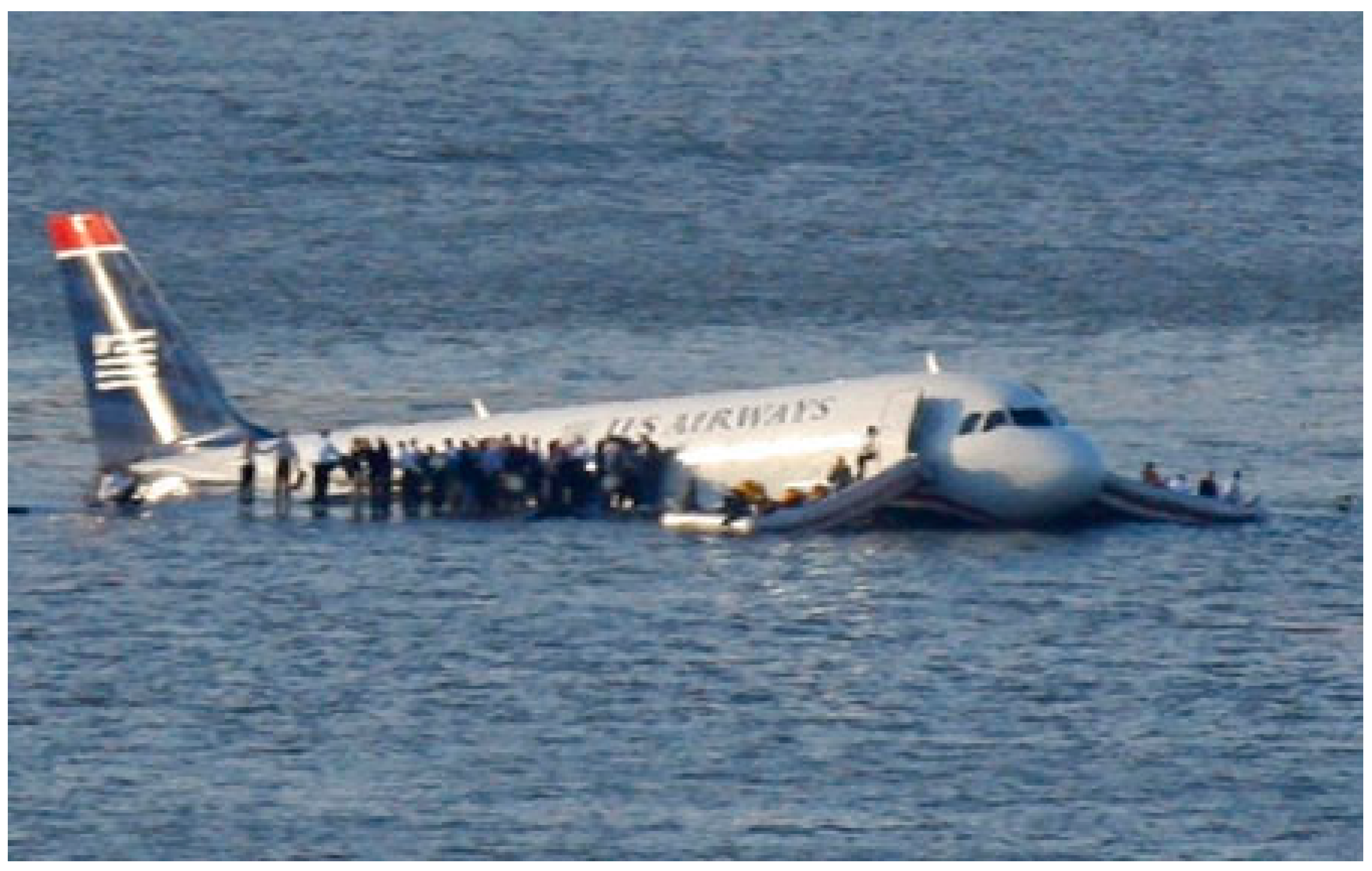
the famous “miracle-on-the-Hudson” event
vs. the infamous UN-shuttle disaster [
10];
- (6)
probability of the flight non-failure if one of the pilots gets incapacitated during the flight [
11];
- (7)
One of the major challenges associated with the application of the PPM concept is the choice of suitable distributions for a particular problem of interest. Although there is no straightforward way for doing that, such distributions could be either based on the accumulated experience or could be anticipated and accepted beforehand based on the common sense and insightful intuition about the physics of the problem. “The intuitive mind is a sacred gift, and the rational mind is a faithful servant. Unfortunately, we have created a society that honors the servant and has forgotten the gift” (A. Einstein). Let us refer, as an example, to the helicopter landing ship (HLS) problem. The actual time of human reaction (decision making) is always positive, is never zero, but could not be unrealistically long either. In addition, shorter times of reaction are more likely than longer times. This means that the probability density distribution function for the human reaction (decision making) time should be skewed towards shorter times, and the most likely time of human reaction (maximum value, mode, of the probability density distribution function) should be low, but never zero. The simplest distribution that meets these requirements is the single-parametric Rayleigh distribution. That is why this distribution was selected to characterize human reaction in the HITL HLS problem. A more powerful and more flexible two parametric Weibull distribution could also be used, but this will make analytical modeling more complicated. As to the lull time in the sea condition, this time is most likely symmetric with respect to its mean value, and therefore the two-parametric normal distribution has been chosen to describe the random lull time. Although, generally, normal distributions cover also negative values of the considered random variable, this “shortcoming” of the distribution is suppressed in our analysis by choosing a large enough ratio of the mean value of lull time to its standard deviation. Another example is the recently suggested double-exponential probability distribution function for the human non-failure, when fulfilling a particular challenging mission in an off-normal situation. This function (addressed in the next section) could be applied in a number of HITL related problems and has also a clear physical meaning. This meaning, as will be shown, is associated with the change in the uncertainty (entropy) of the probability of human non-failure with the change in the level of the mental workload (MWL).
It should be pointed out that while the PPM approach opens new perspectives for aerospace human psychologists and ergonomics specialists, numerous additional analyses will be necessary to make the recommendations and guidelines based on the PPM concept widely accepted and highly practical. These analyses should be geared to various practical situations, including those beyond the aerospace and even vehicular domain.
2. Double-Exponential Probability Distribution Function
“Everyone knows that we live in the era of engineering, however, he rarely realizes that literally all our engineering is based on mathematics and physics”—Bartel Leendert van der Waerden, Dutch mathematician
The probability
of the navigator’s non-failure, when a vehicle is operated in off-normal (extraordinary) conditions, can be assumed to be distributed in accordance with the following double-exponential law of the extreme-value-distribution (EVD) type (see, e.g., [
4]):
here
is the probability of the human non-failure for the specified (normal) mental workload (MWL)
in ordinary (normal) operation conditions;
is the actual (elevated, off-normal) MWL;
is the most likely (normal, specified) human capacity factor (HCF);
is the actual (off-normal) HCF exhibited or required in the extraordinary condition. The
level should be established beforehand, as a function of the normal
and
levels. In avionics this could be done by conducting “accelerated” testing and appropriate measurements on a flight simulator.
By differentiation the Equation (1) with respect to the MWL
we obtain:
where
is the entropy of the distribution
At low MWL levels close to the normal level, the change in the relative probability
of non-failure with the increase in the MWL is significant. This is not surprising though: it is easy to improve a poor performance than a good one. In another extreme case, when the actual MWL
exceeds considerably the normal one
we have:
This result explains the physical meaning of the Equation (1): the change in the probability of human non-failure with the change in the level of the MWL is proportional, for high MWL levels, to the underlying uncertainty (entropy of the distribution of this probability) and is inversely proportional to the MWL level. The right part of the last formula could be viewed as a kind of a coefficient of variation (COV), where the role of the uncertainty in the numerator is played by the entropy, rather than by the standard deviation, and the role of the stressor (MWL) in the denominator is played, as in the well-known statistical COV characteristic, by the MWL, rather than by the mean value of the random characteristic of interest.
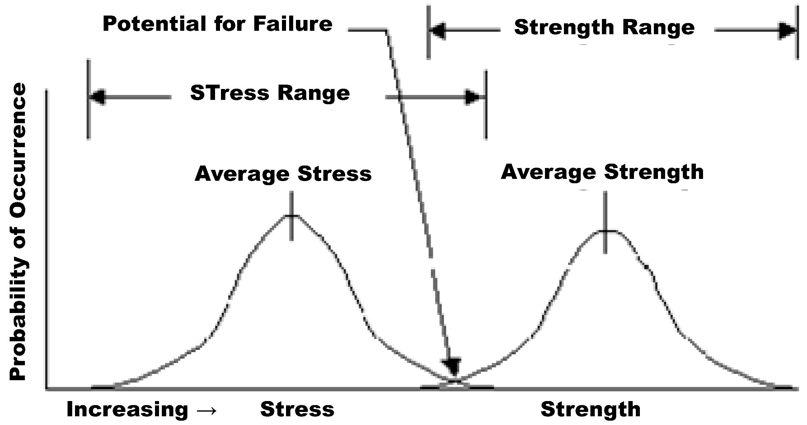
The Equation (1) enables one to quantify, on the probabilistic basis, the human’s ability (capacity) to cope with an elevated mental overload. Using an analogy from the reliability engineering field and particularly with the stress–strength (demand–capacity) interference model (
Figure 1), the MWL could be viewed as a certain demand (stress, load), while the HCF as capacity (strength) of the object. In the case in question it is the capacity of a human to perform the given task. It is the relative levels of the MWL and HCF that determine the human’s “reliability”,
i.e., the likelihood of his/her non-failure (success). Unlike in the well-known capacity-demand interference model, the Equation (1) combines the demand
and the capacity
in the same PPM, with an intent to consider a situation of the type shown in
Figure 2.
Figure 1.
Demand (stress/mental workload (MWL))–capacity (strength/human capacity factor (HCF)) interference curves.
Figure 1.
Demand (stress/mental workload (MWL))–capacity (strength/human capacity factor (HCF)) interference curves.
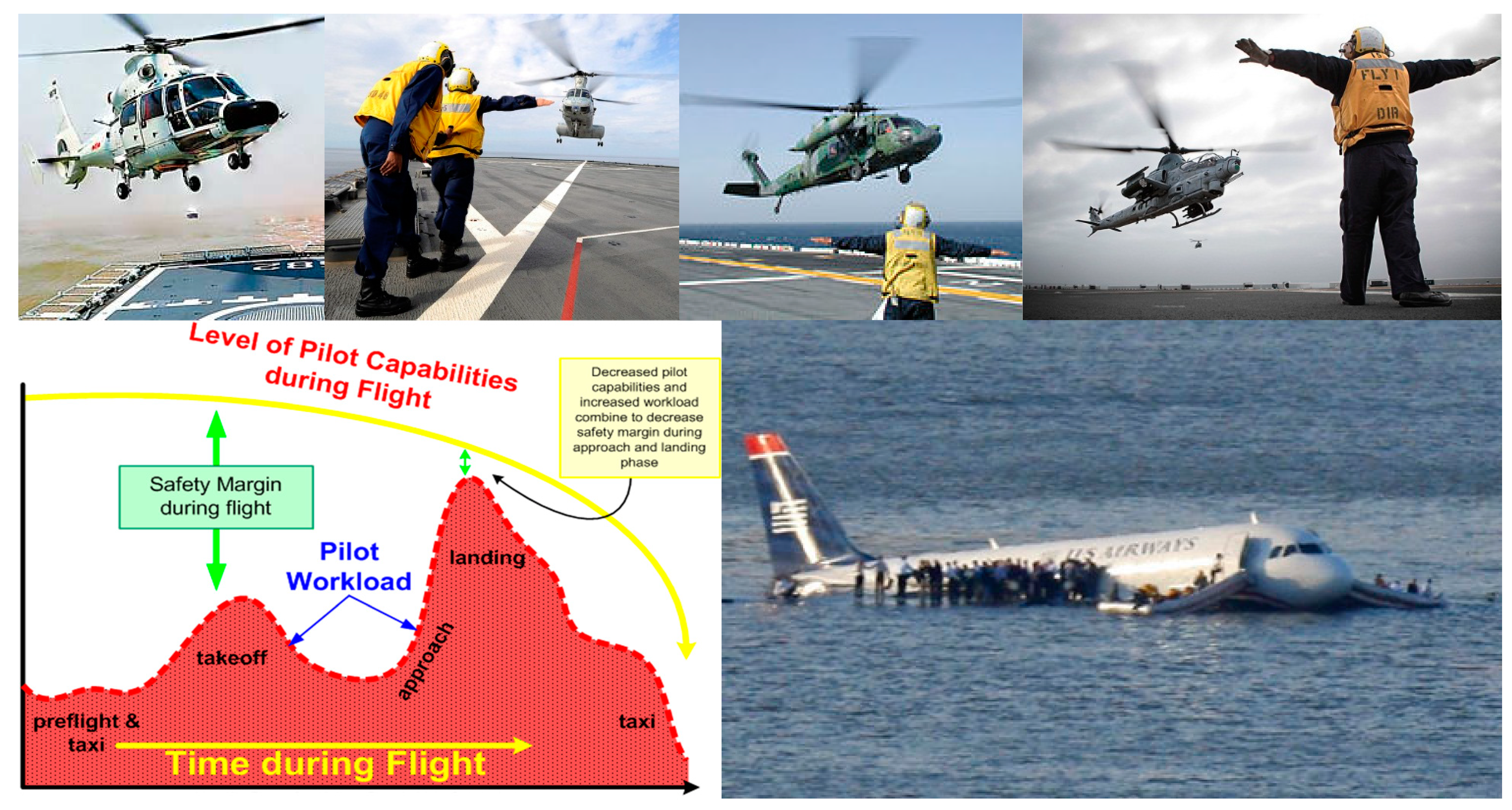
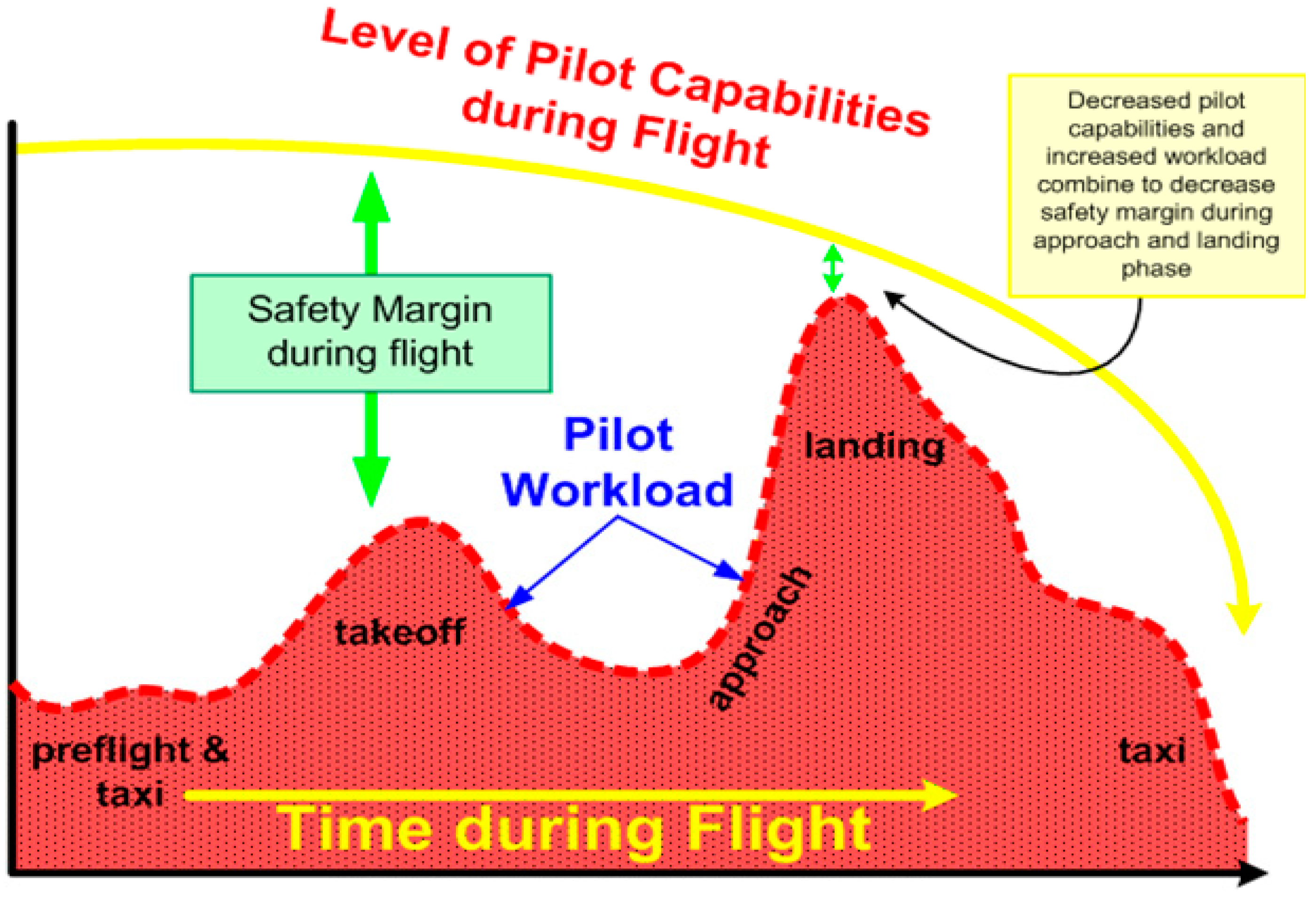
Figure 2.
Long-term (pilot capabilities) HCF vs. MWL (pilot workload).
Figure 2.
Long-term (pilot capabilities) HCF vs. MWL (pilot workload).
It should be emphasized that while the notion of the MWL has been addressed and well described in the human psychology literature, the idea of mental capacity is rather new. Although it is true that it might be difficult to establish a comprehensive list of factors that could impact the HCF and the human performance in a particular situation, it is also true that the MWL has to be compared to a more or less well-substantiated HCF. It goes without saying that MWL and HCF, as a demand and a capacity, are to be measured in the same units, otherwise there will not be possible to create a meaningful “pass/fail” model. The MWL and the HCF could be particularly dimensionless.
Cognitive (mental) overload is central in the today’s aviation and aerospace psychology. Excessive MWL has been recognized for a long time as a significant cause of error in aviation and space navigation. The MWL depends on the operational conditions and the mission complexity, has to do with the significance of the general task and is directly affected by the challenges that a navigator faces, when controlling the vehicle in a complex, heterogeneous, multitask, and uncertain-and-harsh environment. The pilot’s environment includes various concepts of situation awareness: spatial awareness (for instrument displays); system awareness (e.g., for keeping the pilot informed about actions that have been taken by automated systems); and task awareness (that has to do with the attention and task management). Measuring the MWL using subjective and objective measures has become in the today’s aerospace psychology a single key method for improving navigation safety. The subjective ratings are applied particularly during simulation tests. They can be, e.g., in the form of periodic inputs to some kind of data collection device that prompts the pilot to enter a number (say, between 1 and 10) to estimate the MWL every few minutes. A suitable example is heart rate variability. Measurement of cardiac activity has been a useful physiological technique employed for the assessment of MWL, both from tonic variations in heart rate and after treatment of the cardiac signal. Using post-flight questionnaires is yet another approach, because one would not want to interfere with the pilot’s work during actual flight operations.
As to the HCF (capacity), it should consider, but might not be limited to, the relevant human qualities. Examples are psychological suitability for a particular task; professional experience and qualifications; education, both special and general; relevant capabilities and skills; level, quality and timeliness of training; performance sustainability (consistency, predictability); mature (realistic) and independent thinking; independent acting, when necessary; ability to concentrate; ability to anticipate; self-control and ability to act in cold blood in hazardous and even life threatening situations; ability to operate effectively under significant MWL and time pressure; ability to make substantiated decisions in a short period of time; ability to operate effectively, when necessary, in a tireless fashion, for a long period of time (tolerance to stress); team-player attitude, when necessary; swiftness in reaction, when necessary. These and other qualities are certainly of different importance in different HITL situations. It is clear also that different individuals possess these qualities in different degrees even prior to any training. HCF and the corresponding qualities and capacities could be time-dependent. When there is an intent to come up with suitable figures-of-merit (FOM) for the HCF for a particular individual, one could rank, similarly to the MWL estimates, the above and perhaps also other meaningful qualities on the scale from, say, one to ten, and calculate the average FOM for each individual and for a particular task, situation or a mission. Certification of navigators from the standpoint of their HCF could be considered.
The MWL/HCF concept and its possible generalizations (say, by considering time, or multi-parametric MWL conditions), after the appropriate sensitivity analyses (SA) are carried out, can be used:
- (1)
when developing guidelines for personnel training;
- (2)
when choosing the appropriate flight simulation conditions; and/or
- (3)
when there is a need to decide if the existing level of automation and/or the navigation instrumentation/equipment are adequate in extreme, but not impossible, extraordinary situations. If not, additional and/or more advanced instrumentation or equipment should be considered. Then the human participation could be minimized or even eliminated.
The calculated
values indicate that:
- (1)
at normal MWL level and/or at an extraordinarily (exceptionally) high HCF level the probability of human non-failure is close to 100%;
- (2)
if the MWL is exceptionally high, the human will definitely fail, no matter how high his/her HCF is;
- (3)
if the HCF is high, even a significant MWL has a small effect on the probability of non-failure, unless this MWL is exceptionally large (indeed, highly qualified individuals are able to cope better with the off-normal situations);
- (4)
the probability of non-failure decreases with an increase in the MWL (especially for relatively low MWL levels) and increases with an increase in the HCF (especially for relatively low HCF levels);
- (5)
for high HCFs the increase in the MWL level has a much smaller effect on the probabilities of non-failure than for low HCFs.
These intuitively more or less obvious judgments are quantified by using an analysis based on the Equation (1) .The computed data show also that the increase in the HCF
and in the MWL
above the 3.0 has a small effect on the probability of non-failure. This means particularly that the navigator does not have to be trained for an extraordinarily high MWL and to a relative HCF
higher than 3.0 compared to a navigator of an ordinary capacity (qualification). In other words, a navigator does not have to be a superman to successfully cope with a high level MWL, but still has to be trained to be able to cope with a MWL by a factor of three higher than the normal level. As has been mentioned, if the requirements for a particular level of safety are above the HCF for a well educated and well trained human, then the development and employment of the advanced equipment and instrumentation should be considered for a particular task, and the decision of the right way to go should be based on the evaluation, on the probabilistic basis, both the human and the equipment performance.
In conclusion of this section it should be emphasized that although the suggested double-exponential Equation (1) has been found useful and fruitful for the evaluation of the MWL
vs. HCF in different aerospace safety situations, other PPM approaches are also possible and might be quite fruiteful. As Khalil Gibran, famous Lebanese-American poet and writer, had put it, “Say not, ‘I have found the truth’, but rather ‘I have found a truth’”. Such approaches include, but are not limited to, of course, to demand-capacity interference model of the type shown in
Figure 1, including time-dependency of the distributions, as well as various long tailed probability distributions that assign relatively high probabilities to regions far from the modes, means or medians of the underlying distribution considered (see, e.g., [
21]), or, more general, various fractional processes (see, e.g., [
22]). Various EVDs, other than the Equation (1), can also be applied. This is true, particularly, for the widely used in reliability theory Weibull distribution, which can be applied in the HITL problems as well, as shown in the next section of the review.
3. Mission Success and Safety
“There are truths, which are like new lands: the best way to them becomes known only after trying many other ways”—Denis Diderot, French philosopher, art critic, and writer
While the Equation (1) can be used to quantify the likelihood of the human non-failure, the reliability of the equipment (instrumentation), which includes the performance of both the hardware and the software, can be characterized, e.g., by Weibull distribution, which is widely used in reliability engineering. As to the role of the uncertain environment, this could be considered by accounting for the probability of the encounter (occurrence) of a condition of the given level of severity. If appropriate and highly dependable equipment is used, a mission could still be successful, even if the MWL is significant and the HCF is not very high.
The success (failure) of a vehicular mission could be time dependent and could have different actual and specified probabilities of success at different stages (segments). Let, e.g., a particular mission of interest consists of
segments
characterized by different probabilities,
of occurrence of a particular harsh environment or by other extraordinary conditions during the fulfillment of the
i–th segment of the mission. The segments are characterized also by different durations,
and also by different predicted failure rates,
of the equipment and instrumentation. These rates may or may not depend on the environmental conditions, but could be affected by aging/degradation and other time-dependent causes. In the simplified example below we assume that the combined input of the hardware and the software, as far as the failure rate of the equipment and instrumentation is concerned, is evaluated beforehand and is adequately reflected by the appropriate failure rate
values. These values could be either determined from the vendor specifications or, preferably, should be obtained on the basis of the specially designed and conducted failure oriented accelerated testing (FOAT) and subsequent predictive modeling [
14]. FOAT should be preferably geared to a particular predictive model, such as, e.g., multi-parametric Boltzmann–Arrhenius–Zhurkov (BAZ) model [
14]. This model is rather general and flexible and can be successfully employed in many reliability related problems.
The probability of the equipment non-failure at the moment
of time during the fulfillment of the mission on the
i–th segment, assuming that Weibull distribution is applicable, is
where
is an arbitrary moment of time within the
i–th segment, and
is the shape parameter in the Weibull distribution. One could assume that the time-dependent probability of human non-failure can be also represented in the form:
of Weibull distribution, where
is the failure rate,
is the shape parameter and
is the probability of the human non-failure at the initial moment of time
of the given segment. When
the probability of non-failure (say, because of the human fatigue or other causes) tends to zero. The probability
can be assumed particularly in the form of the Equation (1).
The probability of the mission failure at the
i–th segment can be found, in an approximate analysis (in a more rigorous analysis conditional probabilities should be considered) as
and the overall probability of the mission failure can be determined as
This formula can be used also for specifying the failure rates and the HCF in such a way that the overall probability of failure would be adequate for the given mission. The assessments based on the Equation (6) can be used to choose, if possible, an alternative route, so that the set of the probabilities
of encounter of the environmental conditions of the given severity brings the overall probability of the mission failure to an acceptable and low enough level.
Let, for instance, the duration of a particular vehicular mission be 24 h, and the vehicle spends equal times at each of the 6 segments (so that
h at the end of each segment), the failure rates of the equipment and the human performance are independent of the environmental conditions and are, say, λ = 8 × 10
−4 1/h, the shape parameter in the Weibull distribution in both cases is β = 2 (Rayleigh distribution is applicable), the HCF ratio
is
the probability of human non-failure at ordinary conditions is
and the MWL
ratios are 1, 2, 3, 4, 5, and occur with the probabilities
= 0.9530, 0.0399, 0.0050, 0.0010, 0.0006 and 0.0005, depending on the severity of the environmental conditions. These data indicate that about 95% of the mission time takes place in ordinary conditions. The calculated
ratios for the above six segments are 1.0000; 0.9991; 0.9982; 0.9978; 0.9964 and 0.9955. The corresponding computed probabilities
of the human non-failures are 0.9900; 0.9891; 0.9882; 0.9878; 0.9864 and 0.9855; the products
of the equipment and the human non-failures are 0.9900; 0.9891; 0.9882; 0.9878; 0.9864; and 0.9855; and the products
are 0.9435; 0.0395; 0.0049; 0.0010; 0.0006; and 0.0005. With these data the predicted probability of the mission non-failure is:
and the probability of its failure is therefore
5. Helicopter Landing Ship (HLS)
“There is nothing more practical than a good theory.”—Kurt Zadek Lewin, German–American psychologist
The helicopter-landing-ship (HLS) situation [
8,
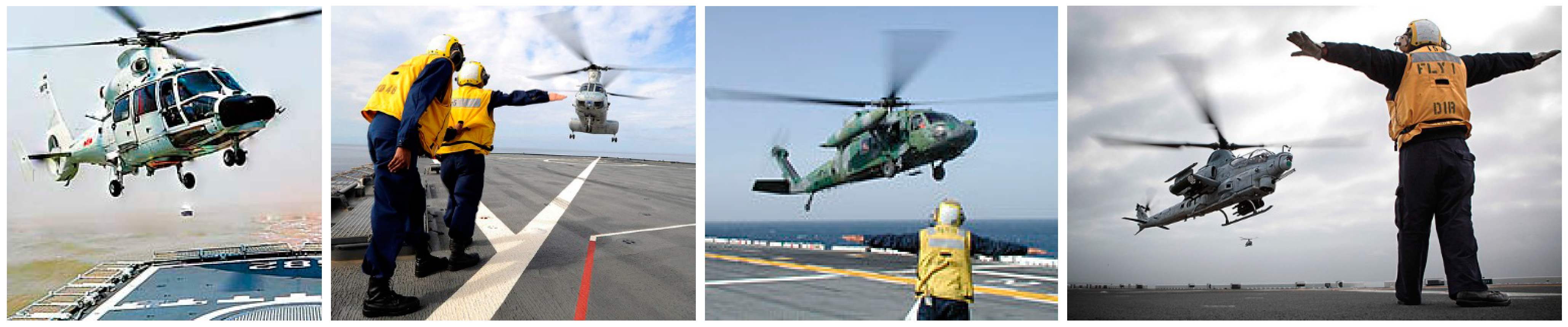
9] is addressed with an emphasis on the human factor role in assuring the helicopter undercarriage strength. This strength should not be compromised as a result of the impact that helicopter experiences during its landing on the ship’s deck. The human factor is important from the standpoint of the operation time that affects the likelihood of safe landing. The operation time includes the time required for the officer-on-board and the helicopter pilot to make their go-ahead decisions, and the time of actual landing. It is assumed in this analysis, for the sake of simplicity, that both these times could be approximated by Rayleigh’s law, while the lull duration follows the normal law with a high ratio of the mean value to the standard deviation. Safe landing could be expected if the probability that it occurs during the lull time is sufficiently high. The probability that the helicopter undercarriage strength is not compromised can be evaluated as a product of the probability that landing occurs during the lull time and the probability that the relative velocity of the helicopter with respect to the ship’s deck at the moment of landing does not exceed the allowable level. This level is supposed to be determined for the helicopter-landing-ground (HLG) situation. The HLG is viewed as a “normal” condition, while the HLS is viewed as an off-normal (extraordinary) situation. The developed PPM can be used when establishing specifications for the helicopter undercarriage strength and when developing guidelines for personnel training. Particularly, the model can be of help when establishing the times to be met by the two humans involved to make their go-ahead decisions in due time to safely land the helicopter.
Typically, officer-on-ship-board, using the information from the on-board surveillance systems, signals to the helicopter pilot, when the lull period (“wave window”) commences (
Figure 3). The challenge is to foresee, the duration of the lull. If the random sum,
T = t + θ, of the random time,
t, needed for the officer-on-board and the helicopter pilot to make their go-ahead decisions, and the random time, θ, needed to actually land the helicopter, is lower, with a high enough probability, than the (random) duration,
L, of the lull, then safe landing becomes likely.
Figure 3.
Helicopter landing ship.
Figure 3.
Helicopter landing ship.
We use Rayleigh’s distributions
as suitable approximations for the times
t and
θ of decision making and actual landing, and the normal distribution
as an appropriate approximation for the duration,
L, of the lull. In the above formulas,
and
are the most likely times of decision making and landing (modes of the corresponding probability density distributions), respectively (in the case of a Rayleigh law these times coincide with the standard deviations of the random variables in question),
is the most likely value (mode) of the lull time (in the case of normal law it coincides with the mean and the median of the distribution), and
is the standard deviation of the lull time. The ratio
(“safety factor”) of the mode to the standard deviation should be large enough (say, larger than 4), so that the normal law could be used as a suitable approximation for the random variable of time that cannot be negative. The probability,
that the random sum
T = t + θ of the variables
t and
θ exceeds a certain level,
can be found as
where
is the error function.
When the most likely duration
of landing is small compared to the most likely time,
required for the officer-on-board and the helicopter pilot to make their go-ahead decisions, the Equation (17) yields:
Thus, the probability that the total time of operation exceeds a certain time duration,
depends in this case only on the most likely time,
of decision making. Solving this relationship for the
ratio, we have:
If the acceptable probability,
of exceeding the time,
is, e.g., P = 10−4, then the total time of making the go-ahead decisions should not exceed 0.233=23.3% of the time,
(lull duration), otherwise the requirement P ≤ 10−4 will be compromised.
Similarly, when the most likely duration,
of decision making is very small compared to the most likely time,
of landing, then
In this case the probability of exceeding time level,
depends only on the most likely time,
of landing.
It is noteworthy that the single-parametric Rayleigh law is characterized by a rather large standard deviation and therefore might provide an over-conservative approximation. A more realistic and more flexible two-parametric law, such as, e.g., Weibull distribution, might be more appropriate and more practical as a suitable probability distribution of the random times, t and θ. Its use, however, will make our analysis unnecessarily more complicated, and our goal is not so much to dot all the i’s and cross all the t’s in the problem in question, but rather to demonstrate that the attempt to use PPM to pre-quantify the role of the human factor in a particular HITL situation is quite fruitful.
When the most likely time
of making the go-ahead decisions and time
of the actual landing are equal, the Equation (17) yields:
For large
ratios
the second term in the brackets becomes large compared to unity, so that only this term should be considered. The calculated probabilities of exceeding a certain time level,
based on the Equation (18), are shown in
Table 1. In the third row of this table we indicate, for the sake of comparison, the probabilities,
P, of exceeding the given time,
when only the time
or only the time
is different from zero,
i.e., for the special case that is mostly remote from the equal time case
Clearly, the probabilities computed for other possible combinations of the times
and
could be found between the calculated probabilities
and
P.The following major conclusions can be drawn from the computed data:
- (1)
the probability that the total time of operation (the time of decision making and the time of landing) exceeds the given time level
rapidly increases with an increase in the time of operation and
- (2)
the probability of exceeding the time level
is considerably higher, when the most likely times of decision making and of landing are finite, and particularly are equal to each other, in comparison with the situation when one of these times is significantly shorter than the other, i.e., zero or next-to-zero.
Table 1.
The probability
that the operation time exceeds a certain time level
vs. the ratio
of this time level to the most likely time
of decision making for the case when the time
and the most likely time
time of actual landing are the same. For the sake of comparison, the probability P of exceeding the time level
when either the time
or the time
are zero, is also indicated.
| 6 | 5 | 4 | 3 | 2 |
|---|
| P* | 6.562 × 10⁻⁴ | 8.553 × 10⁻³ | 6.495 × 10⁻² | 1.914 × 10⁻¹ | 6.837 × 10⁻¹ |
| P | 1.523 × 10⁻⁸ | 0.373 × 10⁻⁵ | 0.335 × 10⁻³ | 1.111 × 10⁻² | 1.353 × 10⁻¹ |
| P*/P | 4.309 × 10⁴ | 2.293 × 10³ | 1.939 × 10² | 1.723 × 101 | 5.053 |
This is especially true for short operation times: the ratio
P*/P of the probability
P* of exceeding the time level
in the case of
to the probability
P of exceeding this level in the cases
or
decreases rapidly with an increase in the time of operation. Thus, there exists a significant incentive for reducing the operation time. The importance of this intuitively obvious fact is quantitatively assessed by the
Table 1 data.
The
Table 1 data can be used, particularly, to train the human for a quick reaction in the HLS situation. If, for instance, the expected duration of the lull is 30 s, and the specified probability of exceeding this time is
then, as evident from the table data, the times for decision making and actual landing should not exceed 5.04 s each. Another useful information that could be drawn from the calculated data is whether it is possible at all to train a human to react in just a couple of seconds. If not, then one should decide on a broader involvement of more sophisticated, more powerful and more expensive equipment to do the job. If pursuing such an effort is decided upon, then developed PPM and extensive probabilistic SA based on this model will be needed to determine the most effective ways to go.
The probability that the normally distributed lull time
L is found below a certain level
is
The probability that the lull time is exceeded can be determined by equating the times
and computing the product
of the probability,
that the time of operation exceeds a certain level,
T, and the probability,
that the duration of the lull is shorter than the time
T. The Equation (19) considers the role of the sea condition (through the values of the most likely duration,
of the random lull time,
L, and its standard deviation,
), the role of the human factor,
(the total most likely time required for the officer-on-ship-board and the helicopter pilot to make their go-ahead decisions for landing), and the role of the most likely time,
of actual landing (which characterizes both the qualification of the helicopter pilot and the qualities/behavior of the flying machine) on the probability of safe landing.
After a low enough allowable value,
of the probability,
is agreed upon, one could establish the allowable maximum most likely time,
of landing. The actual time of landing can be assessed as
where
is the allowable probability that the level
is exceeded. If, for instance,
and
then
s.
The cumulative probability distribution function for the extreme vertical ship velocity
(the probability that the vertical velocity of the ship deck at the HLS location is below a certain level
due to her motions in heave, pitch and roll in waves can be expressed, using the extreme value distribution (EVD) technique. This technique leads to the following distribution:
Here
is the variance of the ship’s vertical velocity
is the expected number of ship oscillations during the landing time
and
is the effective period of the ship motions in irregular seas. The formula
reflects an assumption that a ship in irregular waves behaves as a narrow-band filter that enhances the oscillations whose frequencies are close to the ship’s own natural frequency (in still water) in heave and pitch and suppresses all the other frequencies. If the landing time (measured by the expected number
of ship oscillations) is significant, the second term in Equation (21) becomes small and can be omitted. If the level
is zero, the function
becomes
and, for a high enough
value, we still obtain
If, however, for a finite
(which is never zero and cannot be smaller than one) the level
is high, the function
becomes
The landing velocity,
V, when landing on a solid ground, is a random variable that could be assumed to be normally distributed:
where
is the mean value of the velocity
V and
is its variance. Then the probability distribution function of this velocity (
i.e., the probability that the random velocity
V is below a certain value
v) is
The allowable level
of the landing velocity
V, assuming a large enough probability
can be found from the Equation (23) by substituting the
value with the
value. The cumulative distribution function for the relative vertical velocity
of the helicopter with respect to the ship’s deck can be determined as:
Here
is the variable of integration;
is the safety factor associated with the ship motion, which is computed as the difference between the total safety factor
when landing in rough seas on the ship’s deck, and the safety factor
when landing on the solid ground; and
is the ratio of the variance,
of the relative velocity,
of the helicopter undercarriage with respect to the ship’s deck to the variance ,
of the ship’s vertical velocity
The Equation (24) determines the probability that the random relative velocity,
, of the helicopter undercarriage with respect to the ship’s deck remains below a certain value,
When
(significant ship motions) and/or
(insignificant absolute vertical velocities of the helicopter), the ratio
This situation is unfavorable for the undercarriage strength: the probability that the extreme vertical velocity of the helicopter during its landing on the ship’s deck remains below a certain
value is zero:
For large enough (but not very large)
values (landing lasts for a rather long time), the Equation (24) yields:
For very large
values we have:
Such a situation is also unfavorable for safe landing. For not very large
values, however (landing does not take long), but large
ratios (significant variance of the relative velocity, but insignificant variance of the velocity of the vertical ship motions), the Equation (25) yields:
This formula is not (and should not be) different from the formula for the case of safe landing on a solid ground. For small
ratios (but still large
values), the Equation (26) yields:
This formula contains a factor
that accounts for the finite duration of landing. When
is small (very short time of landing), the situation is not different from the case of landing on a solid ground. When
is large, the situation is certainly unfavorable:
Thus, the probability that a certain level
of the relative velocity
of the helicopter with respect to the ship’s deck is not exceeded can be found as
The probability
that the undercarriage strength will not be compromised can be evaluated as a product of the probability 1 −
PA that the helicopter will be able to land during the lull time and the probability
that the relative velocity of the helicopter with respect to the ship’s deck will not exceed a certain allowable (specified) level
If the landing velocity,
on the ground is treated as a deterministic value (if the variance
of this velocity can be considered zero) and the allowable relative velocity
(which is due to the undercarriage structure only) are known, then the condition of safe landing becomes quite simple. Indeed, in such a situation the Equation (26) results in the following simple formula for the extreme value
of the ship’s vertical velocity:
and the condition of safe landing becomes
Let the most likely times of making the go-ahead decisions and of the actual landing be the same and equal to
t0 = θ
0 = 10 s, the most likely (mean) lull time be
l0 = 20 s, and the standard deviation of the lull time be σ = 5 s. The calculated data are shown in
Table 2. As evident from the table data, the probability
that the time of operations exceeds the duration of the lull increases rapidly with the decrease in the ratio of the lull duration to the most likely time of either the decision making or the landing process, while the probability that the lull duration is below a certain value decreases with the decrease in the ratio of this value to the most likely lull duration. The first effect prevails, and the product of these two probabilities (defining the likelihood that the helicopter is not successful in landing on the ship’s deck during the lull time) increases with the decrease in the duration of the lull time almost as fast as the probability of the operation time does. It is only for very long times of operation that the probability
of exceeding a certain time limit starts to play an appreciable role. We conclude therefore that in the situation in question the human factor associated with the decision making times plays a significant role, as far as safe landing is concerned. The developed model enables one to quantitatively assess this intuitively obvious role.
Let, for instance, the number of ship oscillations during the time of landing be
the required (specified) probability of safe landing be as high as
the variance of the vertical velocity of the ship due to her motions during the lull period be
m/s, and the extreme value of the relative vertical velocity computed as the difference between the specified (allowable) velocity
of the helicopter and the actual ground landing velocity
be
m/s. Then the level of the relative velocity at the moment of landing is:
Hence, landing in this case can be permitted and is expected to be safe.
It could be concluded the PPM approach enables one to quantify the role of the human factor, along with other uncertainty sources, in the HLS situation. Safe landing can be expected if the probability that it takes place during the lull time is sufficiently high.
Table 2.
The probability
of safe landing vs. the ratio
of the normally distributed duration
of the lull to the most likely time
of decision making or the most likely time
of actual landing, when the times
and
are equal.
Table 2.
The probability
of safe landing vs. the ratio
of the normally distributed duration
of the lull to the most likely time
of decision making or the most likely time
of actual landing, when the times
and
are equal.
| 6 | 5 | 4 | 3 | 2 |
|---|
| 6.562 × 10⁻⁴ | 8.553 × 10⁻³ | 6.495 × 10⁻² | 1.914 × 10⁻¹ | 6.837 × 10⁻¹ |
| 3.0 | 2.5 | 2.0 | 1.5 | 1.0 |
| 1.0 | 1.0 | 0.9999 | 0.9770 | 0.5000 |
| 6.562 × 10⁻⁴ | 8.553 × 10⁻³ | 6.494 × 10⁻² | 1.870 × 10⁻¹ | 3.418 × 10⁻¹ |
7. Two Men in a Cockpit: Probability of Non-Failure if One of Them Gets Incapacitated
“I will not take up your time, dear boy, with telling you what is the matter with me. Life is brief, and you might pass away before I had finished”—Jerome K. Jerome, English writer and humorist, “Three Men in a Boat (to say nothing of the dog)”
We apply the modified double-exponential Equation (1)
to a situation, when one of the two equally and highly qualified pilots becomes, for one reason or another, incapacitated at a certain moment of time in the flight (such a mishap is referred to as an
accident), and, because of that, his mate has to cope with a total, say, twice-as-high, MWL [
13]. It does not actually have to be a twice-as-high MWL, but we have chosen this number for the sake of simplicity. In the above formula,
is the probability of failure of the pilot to perform his/her duties,
t/
T is the (nonrandom) ratio of the elapsed operation time,
t, to the total duration,
T, of the flight including landing (0 ≤
t ≤
T),
G is the total MWL treated as a non-random variable,
G0 is the most likely (specified) value of the MWL in the ordinary conditions,
F is the HCF (treated as a random variable), and
F0 is the most likely (specified) non-random value of this factor.
The Equation (30) makes physical sense. Indeed, when t = 0 (at the beginning of the flight) and/or when G = 0 (very low MWL) and/or when F→∞ (highly skilled, highly trained and highly effective operator with a high HCF), then the probability
of the navigator’s failure is zero. When t→∞ (vehicle operates for a very long time) and/or G→∞ (the MWL is extremely high), while the HCF F is finite and might be not very high, then the probability
of the operator failure is equal to one.
Examine a situation at the moment
t of time after an aircraft took off. The flight duration is
T. If the MWL
G is evenly distributed between the two pilots, then, using the Equation (30), we write the probability of failure for each pilot as
If at this moment of time an
accident occurs, and, as a result of this, one of the pilots becomes incapacitated, then his mate will have to cope with the entire workload
G, and the probability that he/she fails during the remaining time (
T −
t) can be found as
From Equations (31) and (32) we have:
If the
accident occurs at the last moment
t =
T of the flight, and the MWL
G is not very large (say, because the environmental conditions are favorable and the navigation equipment is adequate and reliable), then both the probabilities
and
become zero: no
casualty could possibly occur. If the accident occurs at the initial moment of time
t = 0, then the Equations (17) and (18) yield:
If, in such a situation, the MWL
G during the flight is high and the HCF
F has a finite value, then the probabilities
and
are equal to one: human failure will definitely occur and, hence, the aircraft casualty will certainly take place. If, however, the total MWL
G is low, while the HCF
F is significant, then the probabilities
and
are equal to zero: no casualty is likely to occur.
A casualty could not possibly occur if one of the following three cases takes place: (1) none of the pilots fails to perform his/her duties, or if (2) the captain fails to perform his/her duties, but the first officer takes over completely and successfully the operation of the aircraft, or if (3) the first officer fails to perform his/her duties, but the captain takes over completely and successfully the operation of the aircraft. The probability of the first event is
The probabilities of the second and the third events are the same and are
The probability of an accident free navigation can be then evaluated as
The probability of a casualty is therefore
If none of the pilots fails
then no accident could possibly occur (
Q = 0). If one of the pilots is unable to cope even with the half of the total workload
then, certainly, he/she will not be able to cope with the total load either, so that
Q = 1 as well, and the probability of a casualty becomes
Q = 1. The probabilities
and
Q are computed as functions of the probability
in
Table 4.
Table 4.
Probabilities of failure at different MWL conditions.
Table 4.
Probabilities of failure at different MWL conditions.
| MWL Conditions |
|---|
| Q1 | 0 | 0.0001 | 0.0005 | 0.001 | 0.005 | 0.05 | 0.10 | 0.20 | 0.30 |
| Q1/2 | 0 | 2.5 × 10⁻⁵ | 0.0001 | 0.0003 | 0.00125 | 0.01274 | 0.0260 | 0.0543 | 0.0853 |
| Q | 0 | 4.4 × 10⁻⁹ | 8.75 × 10⁻⁸ | 5.25 × 10⁻⁷ | 1.09 × 10⁻⁵ | 0.00111 | 0.00452 | 0.01877 | 0.0439 |
| Q1 | 0.4 | 0.50 | 0.60 | 0.70 | 0.80 | 0.85 | 0.90 | 0.95 | 1.00 |
| Q1/2 | 0.1199 | 0.1591 | 0.2047 | 0.2599 | 0.3313 | 0.3777 | 0.4377 | 0.6239 | 1.00 |
| Q | 0.0815 | 0.1338 | 0.2037 | 0.2963 | 0.4203 | 0.4994 | 0.5963 | 0.7961 | 1.00 |
The following conclusions could be drawn from the computed data: (1) The probability of a casualty is considerably lower than the probability of an accident,
i.e., the failure of one of the pilots to cope with the total workload, especially when the latter probability is low. If one wants to keep the probability of a casualty below, say, 10−5 = 0.001%, then the probability that one of the pilots cannot cope, if necessary, with the entire workload should be kept below 0.5%. If the latter probability is 10%, then the probability of a casualty becomes as high as 0.45%; (2) The probability of a casualty is lower than the probability of failure of one of the pilots to cope with a half of the workload, if the probability of failure of one of the pilots to cope with a total workload is below
and is higher than the probability of failure of one of the pilots to cope with a half of the workload, if the probability of failure of one of the pilots to cope with a total workload is higher than the above number. Certainly, there is a strong incentive to make the probability of failure of each pilot at ordinary conditions as low as possible. The
Table 3 data enable one to quantify this obvious conclusion; (3) The probability that one of the pilots becomes unable to cope with the total workload is always higher, of course, than the probability than he/she becomes incapable to cope with half of the workload. This difference is especially high for low probabilities of failure.
From Equation (32) we find
If the accident occurred when
t/
T = 0.5, and the “force majeure” MWL
G is twice as high as the ordinary (specified) MWL
G0, then
If, for instance,
then
F/
F0 = 3.49. Hence, the extraordinary (“force majeure”) HCF should be about 3.5 fold larger than the ordinary value of this factor. If one requires that the probability of failure is
then the required predicted
F/
F0 ratio should be as high as
F/
F0 = 4.10. In a hypothetical situation, when the accident occurs at the initial moment of time and the pilot and the controller decide nevertheless to continue the flight, the last formula yields:
For
and
we obtain F/F0 = 3.59 and F/F0 = 4.18, respectively. Hence, the time of an accident has a relatively small effect on the increase in the “force majeure” human factor.
In order to assess the role of the time moment, when an accident occurs, examine the following problem. If the casualty did not occur during the time t, what is the probability Q* that it will occur during the remaining time (T – t) of the flight, if the specified probability of the occurrence of the casualty for the entire flight is Q? Two events have to take place in order that the accident occurs during the time (T – t): (1) it should not occur during the time t and (2) has to occur during the time (T – t).The probability that the casualty occurs during the time t is Q(t/T). The probability that the casualty occurs during the remaining time (T – t), provided that it did not occur during the time t, is (1 − Q(t/T))Q*. The probability that the casualty occurs during the total time T can be found as Q = Q(t/T) − (1 − Q(t/T))Q*. Hence,
and
The computed Q* values indicate that the probability Q* that the casualty occurs during the remaining time (T – t) of the flight if it did not occur during the initial time t of the flight is always smaller than the specified probability Q of the casualty occurrence during the total flight time T, and decreases with an increase in the total flight time. At the last moment t = T the probability Q* is zero no matter how high the probability Q is, unless the latter probability is equal to one. The probability Q* increases with an increase in the specified probability Q. the two probabilities coincide at the initial moment of time t = 0; if one wants to keep the probability Q* at a sufficiently low level he/she should keep the specified probability Q also at a low level.
8. Anticipation in Aviation
“You can see a lot by observing”—Yogi Berra, American baseball player; “It is easy to see. It is hard to foresee”—Benjamin Franklin, American scientist and statesman
Anticipation is an important cognitive resource for improved aeronautics safety [
12,
13,
14,
15,
16,
17,
18,
19,
20,
21,
22]. Two problems that have to do with uncertainties in an anticipation effort in aeronautics are addressed in this analysis:
- (1)
assessment of the probability that the random actual (“subjective”, “internal”, pilot-performance-related) anticipation time is below an also random (“objective”, “external”, “available”) time of the dynamic process of interest (if this is the case, it is likely that no-anticipation-related casualty is possible), and
- (2)
evaluation of the likelihood of success of a (random) short-term anticipation from the predetermined (deterministic) long-term anticipation.
While the today’s HITL related efforts in anticipation concepts in aviation are, as a rule, statistical, our approach is based on the PPM. This approach can do what the routine conventional methods cannot: one will not be able to ever accumulate enough statistics on real or near-real disasters coming from “operator error” in an attempt to extract usable design guidelines.
Plenty of insightful analyses have been conducted in the anticipation in avionics field by a number of outstanding cognitive engineers. Employing the traditional approach, when a cognitive engineer starts with an experimental effort and then tries to replicate the findings through simulation, Amalberti [
16] has indicated particularly that no matter how valuable experimentations might be, it is usually next-to-impossible to isolate the role that an inadequate anticipation might play in a particular off-normal situation that led or could have led to a casualty, although some occurred or avoided accidents show that anticipation played the major role. In connection with this finding, we would like to emphasize that such an isolation (separation) could be done, with a greater or lesser success, by using PPM. It is true, of course, that even by using either the traditional approach (experimentation first) or our PPM approach (modeling first) it might still be impossible to correctly identify and consider the role of anticipation and it various aspects, but it would be a miracle, if this could be done by using only one of these two available approaches. The analytical PPM used in the analyses below is of particular importance, since it leads to close form solutions that clearly indicate the role of the major factors affecting the outcome in the problem of interest. In addition, analytical models and formalisms are highly “generalizable”,
i.e., can be used for rather different cognitive engineering related situations, both within a particular domain of application and across various domains.
Two anticipation related problems in aeronautics have been considered in this paper.
One problem has to do with the duration of the anticipation effort as compared to the “available” time until the event of important commences. While anticipation is defined differently in different fields of human psychology, we proceed, following Cellier [
17], from the definition that anticipation is “an activity consisting of evaluating the future state of a dynamic process, determining the time and timing of actions to undertake on the basis of a representation of the process in the future and, finally, mentally evaluating the possibilities of these actions”. In accordance with this definition, one has to assess, on the probabilistic basis, the durations of the following three time periods affecting the success of the anticipation effort:
- (1)
time required to evaluate the future state of the dynamic process of interest (what will most likely happen, if I do not interfere?);
- (2)
time required to determine the time when pilot’s actions should start and what kind of actions should be taken (when should I start acting, and what exactly should I do in view of what might happen if I do not act?); and
- (3)
time required to determine, by mental evaluation, whether the required actions are possible (are the actions that I intend to undertake possible, and, if they are, will I achieve my objective?). If the likelihood that the total anticipation time will be appreciably below the moment of time when the anticipated situation in the dynamic process is expected to commence is high, then there is a reason to believe that the anticipation effort will be successful.
Another problem addressed is the probabilistic assessment of the success of a short-term anticipation from the known (predetermined and deterministic) long-term anticipation. When solving this problem we proceed from Denecker’s [
13] definition and distinction between short-term (“subsymbolic”) and long-term (“symbolic”) anticipations. According to Denecker, short-term anticipation (STA) relies on reflex loops and is “a low level action” control activity, while long-term anticipation (LTA) relies on the solutions based on the accumulated and analyzed knowledge of the situation of interest and the required adequate modus operandi.
When assessing, on the probabilistic basis, the total anticipation time and particularly that this time exceeds a certain level, we assume that the times required to evaluate the state of the approaching dynamic process of interest, the time required to determine the moment of action and the time to decide what kind of actions should be undertaken could be combined into the phase 1 (evaluation phase) of the anticipation time, while the time required to determine, by mental evaluation, whether the required actions are indeed possible are viewed as the phase 2 of the anticipation time (possibility assessment phase). Such a breakdown seems to be justifiable, since in reality the pilot, in his/her cognitive evaluation of the situation, anticipates most likely concurrently his/her activities associated with the assessment of the significance and the attributes of the future state of the dynamic process of importance and the moment of time that, after the future state of the dynamic process of importance is established, the pilot makes the “now or never” decision.
The time required to determine, by mental evaluation, whether the actions decided upon are indeed possible and will meet the objective comprises the phase 2 (possibility phase) of the anticipation process. If, for one reason or another, one decides on a different breakdown of the anticipation phases, the accepted formalism would still be applicable. Based on the accepted time breakdown, one can use the same formalism as in the above HLS problem. Following the HLS formalism, we use the following rationale.
If the (random) sum T = t + θ of the (random) time, t, needed for the completion of the evaluation phase 1 of the anticipation process and the (random) time, θ, of the possibility assessment phase 2 is lower, with a high enough probability, than the “external”, available (random) time, L, from the beginning of the anticipation process to the beginning of the dynamic process of interest, then the anticipation process could be considered successful. The simplest physically meaningful probability distribution for the random times of interest is Raileigh’s law. The rationale behind such an assumption is the same as in the HLS problem: the times t and θ to complete the phases 1 and 2 of the anticipation process cannot be negative, the likelihood of zero random times t and θ is zero, and so is the likelihood of their very large values, and the most likely times t0 and θ0 of the random times t and θ should be small enough, and should be much closer to zero than to very large values. In the Equation (15), t0 and θ0 are the maximum values of these distributions and, hence, the most likely values of the random times t and θ. The mean times
and
of the variables t and θ are related to the most likely times t0 and θ0 as
The (random) time, L, from the beginning of the anticipation process to the beginning of the dynamic process (event) of importance, has a different physical nature than the anticipation times t and θ. While the times t and θ are “subjective” times that have to do with the swiftness and quality of human anticipation, the random time L is an “objective” (“external”, “available”) time that is independent of the human anticipation. It is natural to assume that the normal law Equation (16) can be used as a suitable approximation for the time, L. In the Equation (16) l0 is the most likely (and also the mean and the median) value of the “external” time L, and σ0 is its standard deviation. The ratio l0/σ0 (“safety factor”) of the mean value of the available time L to its standard deviation should be large enough (say, larger than 4), in order that the normal law could be used as an acceptable approximation for a random variable that cannot be negative, and it is the case in question, when this variable is time. The probability P* that the sum T = t + θ of the random variables t and θ (total anticipation time) exceeds a certain time duration (level)
can be found as a convolution of the distributions Equation (15) of the random variables t and θ and is expressed by the Equation (17). When the time
is zero, it will be always exceeded (P* = 1). When the time
is infinitely long
the probability that this time is exceeded is always zero (P* = 0). When the most likely duration
of the phase 2 of anticipation is very small compared to the most likely duration,
of the phase 1, the Equation (17) yields:
i.e., the probability that the total anticipation time exceeds a certain time duration,
depends only on the most likely time,
of of the first phase. If the acceptable probability P* of exceeding the time
(e.g., the duration of the available time, if this duration is treated as a non-random variable of the level
), is, say,
then the anticipation time should not exceed 0.2330 = 23.3% of the time
(expected duration of the available time), otherwise the requirement
will be compromised. Similarly, when the most likely duration,
of the phase 1 of anticipation effort is very small compared to the most likely time,
of the second phase, the Equation (17) yields:
i.e., the probability of exceeding the time level
depends only on the most likely time,
of the second phase of anticipation.
When the most likely times
and
required to complete the two phases of the anticipation effort are equal, the Equation (17) results in the Equation (18). For large enough
ratios
the second term in the brackets becomes large compared to unity, so that only this term should be considered. The calculated probabilities of exceeding a certain time level
based on the Equation (17), are shown in
Table 1. In the third row of this table we indicate, for the sake of comparison, the probabilities,
of exceeding the given time,
when only the time
or only the time
is different from zero,
i.e., for the special case that is mostly remote from the case
The probabilities computed for other possible combinations of the times
and
could be found between the calculated probabilities
P* and
The
Table 1 data should be interpreted in the problem in question as follows: the probability
P* that the anticipation time exceeds a certain time level
vs. the ratio
of this time level to the most likely time
of anticipation for the case when the most likely time
of the first phase and the most likely time
of the second phase are the same. For the sake of comparison, the probability
of exceeding the time
when either the time
or the time
are zero, is also indicated. The following two practically important conclusions could be drawn from the
Table 1 data:
- (1)
The probability that the total time of anticipation exceeds the given time level
rapidly increases with an increase in the time of anticipation;
- (2)
The probability of exceeding the time level
is considerably higher, when the most likely times of the two phases of anticipation time are finite, and particularly are equal to each other, in comparison with the situation when one of these times is significantly shorter than the other, i.e., zero or next-to-zero. This is especially true for short anticipation times: the ratio
of the probability
of exceeding the time level
in the case of
to the probability
of exceeding this level in the case
or in the case
decreases rapidly with an increase in the duration of anticipation time. Therefore an obvious incentive exists for reducing the total anticipation time. The importance of this intuitively obvious fact is quantitatively assessed in our analysis.
The data of the type shown in
Table 1 can be used, particularly, to train the personnel for a quick reaction, as far as the anticipation process is concerned. If, e.g., the expected duration of the available time is 30 s, and the required (specified) probability of exceeding this time is
(0.1%), then, as evident from the table data, the times for each of the two phases of the anticipation process should not exceed 5.04 s. It is advisable, of course, that these predictions are verified by simulation and by actual best practices. Particularly, one should obtain statistical information, from the accumulated experience, about the available time durations for different practical situations. Another useful information that could be drawn from the data of the type shown in
Table 1 is whether it is possible at all to train a human to react (make a quick and reasonable anticipation) in just several seconds. If not, then one should decide on a broader involvement of more sophisticated, more powerful and more expensive equipment to do the job. If pursuing such an effort is decided upon, then an appropriate SA will be needed to determine the most promising ways to go.
The available time L is a random normally distributed variable, and the probability that this time is found below a certain level
can be determined using the Equation (19). The probability that the available time in the anticipation situation is exceeded can be determined by equating the times
and computing the product
of the probability
that the total time of anticipation exceeds a certain level, T, and the probability
that the duration of the available time is shorter than the time T. The Equation (19) considers the effect of the “objective” situation (through the values of the most likely duration,
of the random available time, L, and its standard deviation
), the role of the human factors
and
(the most likely times of the anticipation process phases; these times characterize the pilot qualifications) on the probability of the success of the anticipation process. After a low enough acceptable value
of the probability
is established (agreed upon), the Equation (19) can be used to establish the allowable maximum most likely time
of the second phase of the anticipation process. The actual time of the second (final) phase of the anticipation process can be assessed by the formula
where
is the allowable probability that the level
is exceeded. If, for instance,
s and
then
s.
Let the most likely times of the two phases of the anticipation process be the same and equal to
t0 = θ
0 = 10 s, the most likely (mean) available time be
l0 = 20 s, and the standard deviation of the available time be σ
0 = 5 s. Then, using the Equations (18) and (19), and the data in
Table 1 we obtain the data shown in
Table 2. As evident from the
Table 2 data, the probability
PA that the total anticipation time exceeds the duration of the available time (failure of the anticipation process) increases rapidly with the decrease in the ratio of the duration of the available time to the most likely time of either of the two phases of the anticipation effort, while the probability that the available time is below a certain value, decreases with the decrease in the ratio of this value to the most likely duration of the available time. The first effect prevails, and the product of these two probabilities (defining the likelihood that the anticipation effort fails) increases with the decrease in the duration of the available time almost as fast as the probability of the anticipation time does. It is only for very long anticipation times that the probability
Pl of exceeding a certain time limit starts to play an appreciable role. We conclude therefore that in the situation in question the human factor associated with the anticipation times play a significant role, as far as the success of the anticipation effort is concerned. The developed model enables one to quantitatively assess in the problem in question this role, along with other uncertainty sources. The success of the anticipation effort can be expected if the probability that it takes place during the available time is sufficiently high. The developed simple and easy-to-use formulas enable one to evaluate this probability. The model can be used particularly when developing guidelines for personnel training. Plenty of additional risk analyses and human psychology related effort will be needed, of course, to make such guidelines practical.
The probabilistic assessment of the success of short-term anticipation from the predetermined long-term anticipation can be carried out based on the double-exponential EVD-type probability distribution function given by the Equation (1). According to Denecker [
13], short-term anticipation (STA) relies on reflex loops and is “a low level action” control activity. Long-term anticipation (LTA) relies on the solutions based on the accumulated and analyzed knowledge of the situation of interest and the required adequate modus operandi. Implementing knowledge enables one to make a long-term projection on a next-to-deterministic basis,
i.e., with a very low risk of failure, while a short-term projection requires skills and ability to act swiftly and adequately in often unpredictable and extraordinary situations. In both cases the appropriate HCF is needed and in both cases the outcome depends to a great extent on the level of the MWL. In the analysis that follows we consider that the STA has its roots in the LTA and that the probability of the STA success depends to a great extent on the groundwork carried out when the LTA strategy and sequence of actions has been developed, as well as on the level and quality of training. “Hard in training, easy in battle”, as the Russian Commander-in-Chief Suvorov put it. Better LTA facilitates STA. In other words, the STA has its roots in the LTA and can be viewed as a deviation from the LTA, when the aircraft is operated in conditions, when STA is required.
In this analysis we assume that the probability of the STA success is distributed in accordance with the following double-exponential law of the extreme-value-distribution (EVD) type:
here
is the probability of success (non-failure) of the LTA effort, which is characterized by the MWL for the specified (normal) LTA MWL level
and the LTA HCF
is the most likely (normal, specified, predetermined and pre-established) LTA MWL;
is the STA MWL;
is the required STA HCF. The
level should be established beforehand, as a function of the
level, when the HCF
This could be done, e.g., by conducting testing, measurements and recordings on a flight simulator. The calculated ratios:
of the probability of the STA success to the probability of the LTA success are shown in
Table 3. The following conclusions are drawn from the calculated data:
- (1)
At normal MWL level
and/or at an extraordinarily (exceptionally) high HCF level
the probability of the STA success is close to 100%.
- (2)
The probabilities of the STA success are always lower than the probabilities of LTA success. This obvious fact is quantified by the calculated data.
- (3)
If the MWL is exceptionally high, the STA effort will definitely fail, no matter how high his/her HCF is.
- (4)
If the HCF is high, even a significant MWL has a small effect on the probability of the STA success, unless this workload is exceptionally large.
- (5)
The probability of STA success decreases with an increase in the MWL (especially for relatively low MWL levels) and increases with an increase in the HCF (especially for relatively low HCF levels). This intuitively obvious fact is quantified by the calculated data.
- (5)
For high HCFs the increase in the MWL level has a much smaller effect on the probabilities of STA success than for low HCFs. All these conclusions make physical sense, of course, but provide a valuable quantitative assessment of the likelihood of the STA success.
The
Table 5 data show that the increase in the
ratio and in the
ratio above the 3.0 value has a small effect on the probability of the STA success. This means particularly that an exceptionally highly qualified pilot does not have to be trained for an extraordinarily high STA-related MWL and does not have to be trained by a factor higher than 3.0 compared to a pilot of ordinary capacity (skills, qualification). In other words, a pilot does not have to be a superman to successfully cope with a high level MWL in STA conditions, but still has to be trained in such a way that, when there is a need, he/she would be able to cope with a STA MWL by a factor of 3.0 higher than the normal level, and his/her STA HCF should be by a factor of 3.0 higher than what is expected of the same person in ordinary (normal) conditions.
Table 5.
Calculated
ratios of the probability
of human non-failure in off-normal conditions to the probability
of non-failure in normal conditions.
Table 5.
Calculated
ratios of the probability
of human non-failure in off-normal conditions to the probability
of non-failure in normal conditions.
| 1 | 2 | 3 | 4 |
|---|
| | | | |
| 1 | 1 | 0.3679 | 0.1353 | 0.0498 |
| 2 | 1 | 0.6922 | 0.4791 | 0.3317 |
| 3 | 1 | 0.8734 | 0.7629 | 0.6663 |
| 4 | 1 | 0.9514 | 0.9052 | 0.8613 |
| 5 | 1 | 0.9819 | 0.9640 | 0.9465 |
| 8 | 1 | 0.9991 | 0.9982 | 0.9978 |
| 10 | 1 | 0.9999 | 0.9998 | 0.9996 |
| ∞ | 1 | 1 | 1 | 1 |
| 5 | 8 | 10 | ∞ |
| | | | |
| 1 | 0.0183 | 9.1188 × 10⁻⁴ | 1.234 × 10⁻⁴ | 0 |
| 2 | 0.2296 | 0.0761 | 0.0365 | 0 |
| 3 | 0.5820 | o.3878 | 0.2958 | 0 |
| 4 | 0.8194 | 0.7057 | 0.6389 | 0 |
| 5 | 0.9294 | 0.8797 | 0.8480 | 0 |
| 8 | 0.9964 | 0.9936 | 0.9918 | 2.5 × 10−40 |
| 10 | 0.9995 | 0.9991 | 0.9989 | 4.4 × 10⁻⁶ |
| ∞ | 1 | 1 | 1 | 1 |
Let us elaborate on the LTA and STA MWL and HCF. Although there is no universally accepted definition of the MWL and how it should/could be evaluated, there is a consensus that suggests that MWL can be conceptualized as the interaction between the structure of systems and tasks, on the one hand, and the capabilities, motivation and state of the human operator, on the other. More specifically, MWL could be defined as the “cost” that an operator incurs as tasks are performed. Given the multidimensional nature of MWL, no single measurement technique can be expected to account for all the important aspects of it. Current research efforts in measuring MWL use psycho-physiological techniques, such as electroencephalographic, cardiac, ocular, and respiration measures in an attempt to identify and predict MWL levels. Measurement of cardiac activity has been the most popular physiological technique employed in the assessment of MWL, both from tonic variations in heart rate and after treatment of the cardiac signal. The authors of this paper intend to develop a methodology and to carry out experiments to measure the LTA and STA workloads.
The HCF includes the person’s professional experience; qualifications; capabilities; skills; training; sustainability; ability to concentrate; ability to operate effectively, in a “tireless” fashion, under pressure, and, if needed, for a long period of time; ability to act as a “team-player;” swiftness of reaction, i.e., all the qualities that would enable him/her to cope with high MWL. In order to come up with suitable figures of merit (FOM) for the HCF, one could rank each of the above and other qualities on a scale from one to ten, and calculate the average FOM for each individual.


