Article

Ensembles for Viticulture Climate Classifications of the Willamette Valley Wine Region

1
Northwest Wine Studies Center, Chemeketa Community College, Salem, OR 97304, USA
2
Department of General and Organic Viticulture, Hochschule Geisenheim University, Von-Lade-Strasse 1, 65366 Geisenheim, Germany
*
Author to whom correspondence should be addressed.
Climate 2021, 9(9), 140; https://doi.org/10.3390/cli9090140
Submission received: 26 July 2021 / Revised: 5 September 2021 / Accepted: 11 September 2021 / Published: 15 September 2021

Abstract

:
Future climate projections provide an opportunity to evaluate cultivar climate classification and preferred styles of wine production for a wine grape growing region. However, ensemble selection must account for downscaled archive model skills and interdependence rather than be arbitrary and subjective. Relatedly, methods for generalizing climate model choice remain uncertain, particularly for identifying optimal ensemble subsets. In this study we consider the complete archive of the thirty-two Coupled Model Intercomparison Project Phase 5 (CMIP5) daily Localized Constructed Analogs (LOCA) downscaled historic datasets and their observational data that were used for downscaling and bias corrections. We apply four model averaging methods to determine optimal ensembles for the computation of six common climate classification indices for the Willamette Valley (WV) American Viticultural Area (AVA). Among the four methods evaluated, elastic-net regularization consistently performed best with identifying optimal ensemble subsets. Variation exists among the optimal ensembles computed for each of the six bioclimatic indices. However, a subset of approximately seven to ten climate models were consistently excluded across all six indices’ ensembles. While specific to the archive and wine region, optimal ensemble sizes were noticeably larger than ensemble sizes commonly employed in published studies. Results are reported such that they can be used by researchers to independently perform analyses involving any one of the six bioclimatic indices throughout the WV AVA while using historic and future LOCA CMIP5 climate projections. The data and methods employed herein are applicable for other wine regions.

1. Introduction

Climate is significant in determining cultivar suitability and the resulting wine profile typical for a wine grape growing region [1,2,3,4]. Temperature and water availability are recognized as two of the most important environmental factors influencing grapevine growth and the subsequent quality of berries and wine [5,6,7,8,9]. Various indices exist to classify viticulture climate [10], and several recent studies have evaluated the impacts of climate change to viticulture using bioclimatic indices and downscaled future climate projections for wine regions (see Table 1).
Quénol et al. [11] highlighted the importance of accounting for model uncertainty when performing studies that involve the application of future climate projections. Model simulations of the future from the Coupled Model Intercomparison Project Phase 5 (CMIP5) [12] archive are no longer necessarily considered as equally likely independent realizations of the future climate [13,14,15,16,17,18]. The models constituting the CMIP5 archive are now recognized as interdependent by virtue of shared codes and the use of similar parameterization schemes and calibration methods [17,19,20]. The assumption of archive model independence results in a multi-model mean that is biased by the duplicative information that is contributed by the similar models. This can confound assessments of model agreement about changes in future climate and alter the statistics of identified correlations. Ignoring model dependence can result in poor accuracy and poor uncertainty quantification. The number of effective models in the archive is conjectured to be less than the number of simulations [17,21,22,23,24] and there is a need not only to better understand weighting strategies that constrain projection uncertainty [15,16,17,18], but also to efficiently and effectively generalize model choice in a manner that selects optimal ensemble subsets for specific applications [24,25].
A common approach to uncertainty quantification of future climate projections is to equally weight a multi-model ensemble, possibly formed by the subjective selection of a subset of the available models, wherein weights are assigned without any consideration of model skill [24]. While a given multi-model mean is generally considered a better choice than any single model [24,25], it is also potentially not optimal relative to alternative multi-model ensemble compositions and weights assignment strategies [13,14,15,16,17,18]. It has been noted that the equal weighted multi-model mean does not necessarily quantify projection uncertainty but rather is simply an uninformed ad hoc measure of ensemble spread [26].
It is now more commonplace to address the epistemic uncertainty associated with model choice by applying methods that account for model skill and interdependence wherein skill is measured by a comparison with observed data [15,16,17]. Weight assignments are further complicated by the learned understanding that individual model skill is dependent upon the modeling objective and study location [17]. For viticulture climate classification of a given area using future climate projections, this implies that weight assignments could vary by the bioclimatic index under consideration.
Sanderson et al. [17] introduced two weight assignment strategies to constrain projection uncertainty, one that accounted for model skill and another that combined the computed skill with an evaluation of model independence. These two approaches have been applied in recent studies [14,15,18]. A few recent studies have also applied Bayesian model averaging (BMA) to assign ensemble weights and constrain projection uncertainty [15,16,18]. BMA is attractive from the perspective that it robustly quantifies model uncertainty and its solution implicitly accounts for model interdependence. However, it is unattractive in that its application is highly compute intensive, and can also be technically challenging to diagnose, relative to most other model calibration strategies [27].
Herger et al. [24] distinguished between approaches that assign continuous weights to the entire ensemble archive with those that are focused on the identification of an ensemble subset. They applied mixed integer quadratic programming to efficiently and flexibly find optimal subsets while accounting for model interdependence. Yang et al. [25] used the Taylor diagram [28] to rank models and subsequently combined the higher performing models using simple averaging to find a nine member multi-model ensemble subset that best characterized the spatiotemporal variability of temperature and precipitation over China. In this study we apply a recent advance for regularizing linear models that is directed at automatic variable selection [29,30,31] to find prediction specific optimal ensemble subsets while simultaneously accounting for model skill and interdependence. Regularization of the ensemble linear model is needed given the thirty-two member multi-model archive we consider in this study and acknowledgment that there are 2 n 1 possible models that involve subsets of n predictors [32]. If n = 32, then there are 4,294,967,295 possible models.
Specification of the selection criteria for the ensemble compositions or the ensemble weights is not common in published studies that report on viticultural climate impact assessments using downscaled CMIP5 ensemble subsets. The arbitrary selection and application of a single model or ensemble subset of downscaled CMIP5 models to quantify future climate impacts is most likely incomplete and suboptimal [24,25]. In this article we apply a directed equal weights strategy similar in design to that performed by Yang et al. [25], the two skill weighting strategies introduced by Sanderson et al. [17], and elastic-net regularization [33] to determine for each method optimal ensemble compositions and weights relevant for the computation of the growing season average temperature (GST) [34], growing degree days (GDD) [1,3], Huglin’s index (HI) [35], cool night index (CI) [36], dryness index (DI) [37], and the Géoviticulture multicriteria climate classification (GMCC) [38] viticultural climate indices for a study region containing the Willamette Valley (WV) American Viticultural Area (AVA).
Heat unit accumulation is important for suitability assessment in that each cultivar has a minimum summed temperature requirement to reach maturity. A late-ripening cultivar will not achieve full ripening in a cool climate and an early ripening cultivar will ripen too quickly in a warm climate. Optimal climate suitability occurs where cultivars ripen at the end of the growing season [8]. The most common applied heat unit accumulation index is the Winkler index (WI), more often referred to as growing degree days (GDD) [1,3,10]. It is the sum of the mean temperatures above a specified base for the growing season, defined as 1 April–31 October in the northern hemisphere [1]. The Huglin index (HI) [35] is similar in form to the GDD method but gives extra weight to the maximum temperature, includes an adjustment factor to account for day length as a function of latitude, and as originally defined only sums for the months April–September. Huglin and Schneider [39] classified cultivars as a function of HI. The GST climate index is the mean of the observed maximum and minimum daily surface air temperature values from the first of April through the end of October (for the Northern Hemisphere). Jones [34] demonstrated broad correlation between the GST and cultivar ripening potential across many wine regions.
While temperature-based heat unit accumulation indices are most used to address viticultural suitability [3], Tonietto and Carbonneau [38] introduced the Géoviticulture multicriteria climate classification system (GMCC) to describe and compare the climates of vineyards worldwide. The GMCC combines three complementary viticulture indices that not only capture climatology but also relate well to qualitative potential and characteristics relevant to wine production. The first index, HI, accounts for heat unit accumulation. The second index is the cool night index (CI) which is defined as the mean of the minimum night temperatures for the month before harvest. The third GMCC index is the dryness index (DI). It is the aggregate vertical accounting of potential soil water availability for April to September whose computation considers precipitation, soil evaporation, and vine transpiration while excluding surface runoff and drainage. It functions as an indicator of the level of presence-absence of dryness for a given area. The GMCC is applicable at multiple spatial scales and includes a comprehensive companion database to support worldwide climatic group comparisons, and one potential use of it is the study of the evolution of viticultural climate as a function of climate change [38].
We consider the complete archive of thirty-two CMIP5 daily Localized Constructed Analogs (LOCA) downscaled historic datasets [40,41] of minimum surface air temperature, maximum surface air temperature, and precipitation (https://gdo-dcp.ucllnl.org/downscaled_cmip_projections/ accessed on 2 December 2020) and their observational data that were used for downscaling and bias correction [42]. The method comparison provides an opportunity to learn about their relative performance. It also reveals optimal ensemble subset sizes for the computation of the GST, GDD, HI, CI, DI, and GMCC indices in the WV AVA. Moreover, by considering multiple indices, we can explore whether LOCA CMIP5 ensemble compositions and weights vary by viticulture climate classification index.
The Willamette Valley is of interest not only given its recent and consistent observed warm to hot vintages [43], but also due to the very limited previous study of climate change impacts to viticulture in the AVA [44]. To our knowledge, this is the first study to comprehensively evaluate a complete downscaled CMIP5 model archive to determine optimal ensemble compositions and weights for the computation of future projections of viticulture climate classification for a wine region. Acknowledging that this type of study is technically challenging and infrequent [24], our results are provided in a manner such that they can be directly used by others to reliably analyze the impacts of daily LOCA CMIP5 future climate projections to viticulture for the WV AVA.

2. Materials and Methods
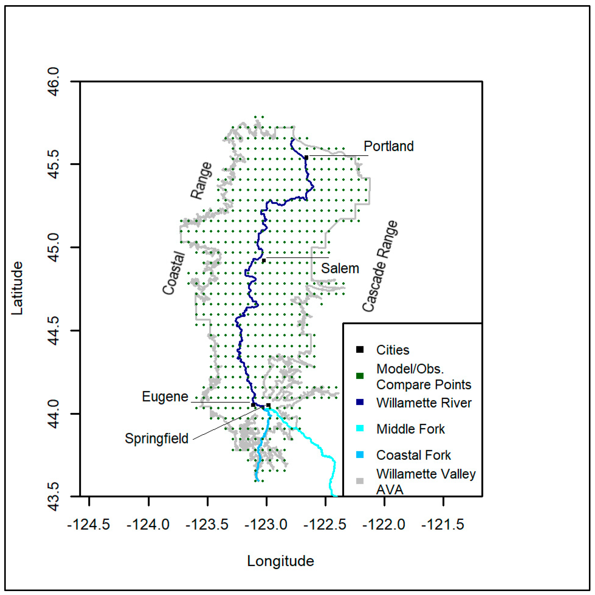
2.1. Study Region

The study region consists of 553 model-observation comparison points which cover the 13,913 square kilometer Willamette Valley AVA which lies in the Willamette River Basin in the northwestern part of the State of Oregon (OR) in the U.S. (Figure 1). The WV AVA includes the entire main stem of the Willamette River, including parts of its Middle Fork and Coastal Fork which join near Springfield, OR just south of Eugene, OR. The Willamette River generally flows in a northly pattern to its confluence with the Columbia River in Portland, OR. The WV AVA is bounded to its west by the Oregon Coastal Range and to its east by the Cascade Range.
The Oregon Wine Board [54] reported for the 2019 vintage 25,197 harvested acres of the WV AVA’s 25,452 planted acres. Total production for the WV AVA was estimated to be 73,560 tons, which accounted for approximately 69.7% of the total wine grape production for the State of Oregon. For the WV AVA, Pinot Noir, Pinot Gris, Chardonnay, Pinot Blanc, and Riesling accounted for 69.3, 16.9, 7.4, 1.2, and 1.2 percent of its total production, respectively.

2.2. Time Series Data

The complete archive of Coupled Model Intercomparison Project phase 5 (CMIP5) daily Localized Constructed Analogs (LOCA) multi-model historic (1950–2005) datasets [40,41] of minimum surface air temperature, maximum surface air temperature, and precipitation was collected from the Downscaled CMIP5 Climate and Hydrology Projections archive at https://gdo-dcp.ucllnl.org/downscaled_cmip_projections/ (accessed on 2 December 2020). The 32 models and modeling groups that provided the data used in this study are listed in Table S1. The observation-based 1/16° longitude-latitude gridded Livneh data product [41] was used to train and downscale the daily LOCA CMIP5 datasets which span 25.125° N to 52.875° N and −124.625° E to −67.000° E [40,55]. In this study, version 1.2 of the Livneh dataset at the 553 grid locations indicated in Figure 1 functioned as the observation dataset. It was processed and compared with its corresponding LOCA CMIP5 processed model historic data counterparts [18] to compute prediction specific (i.e., growing season average temperature (GST), growing degree days (GDD), Huglin index (HI), cool night index (CI), dryness index (DI), and Géoviticulture multicriteria climate classification (GMCC)) model-to-measurement evaluations and resulting ensemble composition and weights.

2.3. Viticulture Climate Indices and Processed Datasets for Prediction Specific Modeling Analyses

Calculation of any one of the six viticulture climate classification indices involves one or more variables wherein each individual variable is a unique processed base model/observation data product (i.e., precipitation, maximum surface air temperature, minimum surface air temperature). The model-observation datasets developed to support the prediction specific modeling analyses were not the specific viticultural climate indices but rather processed datasets that support their calculation as indicated in Equations (1)–(4), (5) and (7). The growing season average temperature, GST [34], growing degree days, GDD [1,3], Huglin index, HI [35], and cool night index, CI [36], are defined in Equations (1)–(4), respectively.
GST = 1 n A p r   1 O c t   31 ( T m a x + T m i n ) / 2 = f ( A p r   1 O c t   31 T m a x , A p r   1 O c t   31 T m i n ) ,
GDD = A p r   1 O c t   31 m a x [ ( ( T m a x ¯ + T m i n ¯ ) / 2 ) 10 , 0 ] = f ( T m a x ¯ , T m i n ¯ ) ,
HI = A p r   1 S e p   30 m a x [ ( ( ( T m e a n ¯ 10 ) + ( T m a x ¯ 10 ) ) / 2 ) , 0 ] · K = f ( T m a x ¯ , T m i n ¯ ) ,
CI = 1 30 S e p   1 S e p   30 T m i n = f ( T m i n ) ,
where n = 214 , T m a x and T m i n , T m a x ¯ , T m i n ¯ , T m e a n ¯ , and K denote the number of days for the northern hemisphere growing season, the maximum and minimum daily surface air temperature data values in °C, the monthly means of the T m a x , the monthly means of the T m i n , the monthly means of the mean of the T m a x and T m i n , and an adjustment factor to account for day length as a function of latitude, respectively. In Equation (1) we see that the GST is a function of the sums of the T m a x and T m i n for the duration of the growing season. Equations (2) and (3) emphasize that the GDD and HI are each a function of the T m a x ¯ and T m i n ¯ for their respective periods. The adjustment factor, K , for the calculation of the HI was not included in the right-hand side of Equation (3) since it does not vary by climate model. The CI is a function of the T m i n for the month of September (see Equation (4)). The dryness index [37] is a function of the April to September monthly means of the daily precipitation and maximum and minimum surface air temperature data,
DI = f ( P ¯ ,   T m a x ¯ ,   T m i n ¯ ) .
It is based on the following equation calculated monthly from April to September,
W = W o + P T v E s ,
where W ,   W o ,   P ,   T v , and E s represent the soil water reserve in millimeters (mm) at the end of a given month, the initial soil water reserve in mm, monthly precipitation in mm, monthly potential transpiration in mm, and monthly direct evaporation from the soil in mm [38]. The value for DI each year is the value of W at the end of September (See [38] for additional details about calculation of the DI). The Géoviticulture multicriteria climate classification (GMCC) is defined as the cross product of the HI, CI, and DI [38]; hence,
GMCC = f ( P ¯ ,   T m a x ¯ ,   T m i n , ¯   C I ) .
Relative individual LOCA CMIP5 model performance may vary across each of a given prediction’s respective functional variables [15,17,18,23]. For example, for computation of the GST, an individual LOCA CMIP5 model might possess better skill relative to the remaining members of the archive in summing daily maximum surface air temperatures from April through October but poor skill relative to the remaining members of the multi-model ensemble with summing the daily minimum surface air temperatures from April through October. Recently introduced methods for evaluating climate model skill require the consideration of each individual variable composing the prediction [15,17,18,23]. Table 2 summarizes the model/observation datasets that were developed to evaluate the performance of LOCA CMIP5 individual and multi-model ensembles for the calculation of the six viticulture climate classification indices throughout the WV AVA. Each processed model-observation dataset specified in Table 2 used data from the 553 model-observation grid locations indicated in Figure 1 for the entire 56 years (1950–2005) that define the LOCA CMIP5 historic period.

2.4. Modeling Averaging Methods

Model averaging involves combining models to improve prediction accuracy and reduce forecast uncertainty, preferably while simultaneously accounting for model skill and interdependence [15,16,25,56]. Eyring et al. [13] expressed the need for further study and better understanding of advanced model averaging methods for climate projections.

2.4.1. Model

The specified model is a general linear model without intercept,
M = i = 1 32 w i M i ,
where M i and w i represent the i -th LOCA CMIP5 model and its assigned non-negative weight, respectively. The modeling objective is to minimize model-to-measurement misfit for each WV AVA viticulture climate classification index directed dataset defined in Table 2 by using one of four different methodologies as they are described in Section 2.4.2, Section 2.4.3, Section 2.4.4, Section 2.4.5.

2.4.2. Skill Weighting

Sanderson et al. [23] and Sanderson et al. [17] introduced a weight assignment strategy for developing climate multi-model ensembles that addressed the assumption regarding CMIP5 model democracy; namely, that individual members of the CMIP5 multi-model archive can vary in their skill by location and prediction. Computation of the root mean squared error (RMSE) between the observations and each model, by variable, enables the ranking of the individual ensemble members. The RMSE is given by
R M S E = 1 N j = 1 N ( S j O j ) 2 ,
where S , O , and N denote modeled data, their observed counterparts, and the number of model-observation comparisons. The skill weight assigned to the i -th LOCA CMIP5 model [17,23] is defined as
w s k i l l , i = A e ( δ i ( o b s ) D q ) 2 ,
where A , δ i ( o b s ) , and D q denote a normalizing constant such that the entire set of individual model skill weights sums to one, the median skill for each model [15], and a parameter called the radius of model equality [23] which determines the degree to which models with poor skill are down-weighted. A model’s median skill is defined as the median of its individual relative RMSE values, E * [15,17,23], where
E * = 1 + E E ¯ E ¯ ,
and E and E ¯ denote, for a given prediction specific functional variable, the model’s RMSE and the mean RMSE across all ensemble members, respectively. A small value assigned to the radius of model equality will result in a weights assignment that favors an ensemble subset whose members possess the best median skill values; whereas, as D q , computed weights will approach the multi-model mean which does not account for model skill.

2.4.3. Skill and Model Interdependence Weighting

Sanderson et al. [23] and Sanderson et al. [17] augmented their skill weight assignment strategy to also account for model similarity in attempts to develop ensemble compositions and weights that further reduce CMIP5 archive redundancy by virtue of shared parameterization schemes and training methods. As with their skill weight assignment strategy, RMSE values calculated between each model and its respective variable specific processed observations enables the calculation of independence weights for each LOCA CMIP5 ensemble member. A multi-variate inter-model distance matrix, δ , is computed as the equally weighted linear combination of normalized variable specific inter-model distance matrices that are each composed of their RMSE distances between each pair of models. For any two models i and j , a similarity score matrix is defined as
S i j = e ( δ i j D u ) 2 ,
where D u is a parameter defined as the radius of similarity which specifies the distance scale over which models should be considered similar and down-weighted for co-dependence. We choose a value of 0.5 for D u [15,23]. In theory, for two identical models, S i j = 1 . Also, S i j 0 as δ i j . Using the similarity scores, the independence weight for the i -th LOCA CMIP5 model is defined as
w u ( i ) = ( 1 + i j n S i j ) 1 ,
where n is the total number of models [15,17,23]. A weight to assign to each individual model that simultaneously accounts for its skill and interdependence is the product of its skill weight and independence weight
w ( i ) = A · w s k i l l , i · w u ( i ) ,
normalized by A such that the sum of the w ( i ) across all models equals one [15,17,23].

2.4.4. Model Median Skill Directed Simple Model Averaging

For each prediction, the median skills computed for each model, δ i ( o b s ) , were ranked and ensembles of size one to size equal to thirty-two were constructed using simple model averaging. This is like the approach presented by Yang et al. [25] who used skill scores obtained from application of the Taylor diagram [28] to build multi-model ensembles using simple model averaging.

2.4.5. Elastic-Net Regularization

In their climate model subset study, Herger et al. [24] mentioned lasso regression from the field of machine learning as an alternative method to their approach. Zou and Hastie [33] introduced the elastic-net penalty as a compromise between ridge [57,58] and lasso [59] regression. Given observations y i ,   i = 1 ,   , n , an n × m matrix of covariates X , and an assumed linear model
y i = η 0 + η 1 x i , 1 + + η m x i , m ,
the elastic-net minimizes
1 2 n i = 1 n w ˜ i ( y i η 0 η x i T ) 2 + λ j = 1 m [ 1 2 ( 1 α ) η j 2 + α | η j | ] ,
where λ is a non-negative regularization parameter that is tuned to weight the overall strength of the penalty, α [ 0 , 1 ] is specified to control the penalty term to vary from ridge regression at α = 0 to lasso regression at α = 1 , and w ˜ i is the weight assigned to the ith observation [29]. Ridge regression yields smooth solutions that include all the predictors, whereas application of lasso regression results in automatic variable selection (i.e., sparse, much more easily interpretable solutions) [32]. The elastic-net combines the two methods. As α increases from 0 to 1 for a fixed λ , the number of zero-valued η j increases from 0 to the sparsity of the lasso [29]. In this study, variable selection was desired, therefore α was specified close to 1 for numerical stability [29]. With α specified close to 1, the elastic-net performs much like lasso regression while retaining ridge regression’s capacity to collectively shrink the coefficients for any highly correlated covariables [29,60]. Cross validation (CV) was employed to ensure that the minimizing value for λ was properly located for each elastic-net application. Google Scholar reports 14,411 citations for [33]. Implementations of the elastic net exist in R, Matlab, Apache Spark, and SAS.

3. Results and Discussion

For each viticulture climate classification directed prediction (i.e., GST, GDD, HI, CI, DI, GMCC), individual LOCA CMIP5 model RMSEs computed by variable are listed in Table 3. Together with the specification of D q and D u , these RMSE values can be used to independently calculate prediction specific ensemble skill weights and independence weights.
Figure 2 presents viticulture climate classification directed LOCA CMIP5 model relative RMSE values, E * , and median skill values, δ i ( o b s ) , also normalized such that their means are one. Each row of Figure 2 has its own color scale wherein its minimum, mean, and maximum are blue, white, and red, respectively. Hence, for any given row, models color coded with shades of blue/red possess more/less skill than the ensemble mean. The first two/third and fourth/fifth and sixth/fifth through seventh/fifth through eighth rows of Figure 2 are the variables specific for the calculation of the GST/GDD/HI/DI/GMCC, respectively. The ninth through fourteenth rows of Figure 2 are the computed median skill values for calculation of the GST, GDD, HI, CI, DI, and GMCC, respectively.
LOCA CMIP5 model median skill values vary by model and their individual rankings differ for each of the six viticulture climate classification indices that were considered for the Willamette Valley AVA. The results not only emphasize that it is necessary to account for model skill, but also, considering Equation (10), that skill weight assignments are prediction specific [17,23]. Model median skill values, δ i ( o b s ) , are a function of their related relative RMSE values, E * . The results presented in Figure 2 also emphasize that individual model skill varies for each of the functional variables relevant for the calculation of the GST, GDD, HI, CI, DI, and GMCC, respectively. For example, for calculation of the GST, its related relative RMSE model rankings emphasize that individual models substantively differ in their relative capacities to sum the daily (1) maximum and (2) minimum surface air temperatures from the beginning of April to the end of October.
Despite the previously mentioned observed differences with LOCA CMIP5 individual model skill for the calculation of six specific viticulture climate classification indices throughout the WV AVA, some observed similarities also exist. A strong consistency is observed for the rankings of model median skill values, and their related relative RMSE values, E * , for the GDD and HI, which is understandable given their similar functional variable definitions (see Equations (2) and (3), and Table 2). In addition, across all six viticulture climate classification indices, there exists a group of nine LOCA CMIP5 models (bcc-csm1-1-m, CanESM2, CCSM4, CMCC-CM, CMCC-CMS, CNRM-CM5, CSIRO-Mk3-6-0, EC-EARTH, and MPI-ESM-MR) the median skill of which, in each case, is consistently greater than its ensemble mean.
Figure 3 is the multi-variate inter-model distance matrix that was developed using the RMSE values listed in Table 3 that are relevant for calculation of the GMCC viticulture climate classification index throughout the WV AVA. Together with specification of the radius of similarity, this matrix supports computation of model independence weights to account for, in addition to skill, archive model interdependence by down-weighting similar models [15,17,18,23]. Multi-variate inter-model distance matrices were also computed to calculate independence weights for the five other viticulture climate classification indices. In Figure 3, model pairs with small inter-model distances are denoted blue and considered dependent, whereas larger pairwise inter-model distances are red and signify independent models.
For all six viticulture climate classification indices considered in this study, calculated independence weights did not substantively alter results that were obtained which solely considered model skill weighting (see Table 4). This observation agrees with results presented by Wootten et al. [18]. Figure 4 is a plot of normalized independence weights that were calculated for each of the six viticulture climate classification indices. The normalized independence weights shown in Figure 4 emphasize that Equation (13) does not sufficiently down-weight model redundancy and only provides a slight nudge to weight the independent models more heavily. For this study, the slightly more heavily weighted independent models in general were also the models with poor relative skill. The skill as well as skill model interdependence weighting schemes generally produce weight assignments that cluster together [18].
Viticulture climate classification directed LOCA CMIP5 model median skill values, δ i ( o b s ) , directly computed from the RMSE values listed in Table 3 and graphically represented in Figure 2, were ranked to develop ensemble compositions of size one to thirty-two. For each prediction of interest (i.e., GST, GDD, HI, CI, DI, and GMCC), the RMSE was subsequently computed for each of these thirty-two model compositions using simple model averaging (see Figure 5 for GST and Figures S1–S5 for GDD, HI, CI, DI, and GMCC, respectively). As previously mentioned, this simple method is like the approach presented by Yang et al. [25]; however, instead of the ranked skill scores from the Taylor diagram [28] we used the ranked model median skills.
Figure 5 includes a plot of the RMSEs computed using simple model averaging (SMA) for each of the thirty-two ensemble compositions formed from the ranked median skill values that are of relevance for the calculation of the growing season average temperature, GST, throughout the WV AVA. This median skill directed SMA plot demonstrates a quick drop from its single model RMSE to a minimum, associated with an ensemble subset of size 10, and subsequently rises to the ensemble mean composed of all thirty-two models. This pattern is generally also observed in Figures S1–S5; however, the ensemble sizes associated with the minimum RMSE for prediction of the GDD, HI, CI, DI, and GMCC are 11, 18, 12, 14, and 21, respectively.
Figure 5 and Figure S1–S5 also include results from application of the skill weighting method [17,23], with each figure including results associated with different parameterizations (i.e., values for the radius of model equality) that effectively result in ensemble compositions of varying sizes when zero is defined for a computed weight with a value less than 1 × 10⁻⁴ to estimate ensemble size for the given D q value. In each figure, as the radius of model equality is increased from its initially assigned value which yields the most parsimonious ensemble composition considered for the skill weighting method, RMSE values for the skill weighting ensembles drop to a minimum and subsequently rise toward the no skill ensemble mean. For the skill weighting method, its minimum is always composed of all 32 models (see Figure 5 and Figure S1–S5).
Herger et al. [24] emphasized that the skill and model interdependence weighting methods are directed at assigning continuous weights as opposed to the identification of optimal ensemble subsets. Results presented herein and also by Wootten et al. [18] reinforce this observation (see Figure 5 and Figure S1–S5 and Table 4). However, it is notable to observe that the model median skill directed simple model averaging method generally yields lower RMSE values than those computed from the skill weighting method for ensembles of comparable sizes (see Figure 5 and Figure S1–S5). The method also consistently finds an optimal ensemble subset with an RMSE value less than or equal in value to the skill weighting method minimizing RMSE that includes the complete archive (see Figure 5 and Figure S1–S5).
While relatively straightforward methods such as skill weighting, skill weighting including interdependence, and model median skill SMA can be proposed and applied to assign weights for model averaging, one can instead apply optimization and inference methods that involve a systematic and iterative search of parameter space, including implementation of formal stopping/convergence criteria, to find prediction specific optimal ensemble compositions and weights to account for skill and interdependence. For example, Massoud et al. [15], Massoud et al. [16], and Wootten et al. [18] applied BMA [61], which involves Markov Chain Monte Carlo sampling, and Herger et al. [24] employed mixed integer quadratic programming for model averaging. We apply a calibration method that to our knowledge has not previously been considered for combining multi-model climate projections; viz., the elastic-net penalty [33]. It can be readily configured to either find smooth solutions or parsimonious models while preserving fit with the observational dataset.
Figure 5 and Figure S1–S5 further include results from applications of elastic-net regularization configured for automatic variable selection. Each elastic-net application was performed using the R software package ‘glmnet’ [29], employing k -fold CV with k = 32 (i.e., leave-one-out CV), α = 0.95 , and w ˜ i = 1 for each observation. The best regularizing model is defined to be at the largest λ value within one standard error of the minimum [29,60,62]. Each figure includes the minimum, identified using leave-one-out cross validation, and its associated best regularized solution. The best regularized solution in each case differed only slightly from the minimizing solution. Elastic-net regularization consistently found a minimizing optimal ensemble subset that outperformed the other three model averaging methods considered in this study (see Figure 5 and Figure S1–S5). From a practical perspective, for a given prediction, application of elastic-net regularization is less resource and time intensive to apply than the skill weighting, skill and model interdependence weighting, and the model median skill SMA methods.
The calibrated models listed in Table 5 are prediction specific (i.e., GST, GDD, HI, CI, DI, GMCC) weight assignments computed from cross validation directed applications of elastic-net regularization configured for automatic variable selection. Equation (8) can be applied using the weights listed in Table 5 to optimally compute, within the framework presented herein, the GST, GDD, HI, CI, DI, or GMCC for the WV AVA while using LOCA CMIP5 historical and future climate projections. For example, the T m a x and T m i n associated with the ensemble model M defined using the weights listed in the second column of Table 5 can be used to optimally compute the GST throughout the WV AVA using Equation (1). The model weights listed in Table 5 are based on comparisons with the Livneh dataset [42] for the LOCA CMIP5 defined historical period [40,41]. While not shown, closely matching summary statistics were also obtained for each respective viticulture climate index, for calibration and verification, from cross validation directed elastic-net regularization fits which held back twenty-five percent of the LOCA CMIP5 historical data.
The models listed in Table 5 for optimized computation of the GST, GDD, HI, CI, DI, and GMCC throughout the WV AVA further reinforce statements regarding CMIP5 archive democracy and redundancy [15,16,17], and the need to develop ensemble compositions and weights assignments for a specific modeling objective and location [17]. For each viticulture climate classification index, unique ensemble subsets with variable sizes and weights were identified which outperform the complete archive ensemble mean in each case. Table 6 summarizes computed correlations among the models listed in Table 5. The optimal ensembles identified for the GST and CI viticulture climate classification indices both demonstrate poor correlation with the remaining four indices. Strong correlations exist among the optimal ensembles identified for computation of the GDD, HI, DI, and GMCC indices for the WV AVA when w ˜ i = 1 for each observation. The general functional definitions for the GST and the CI are each unique relative to the remaining four indices which share common variables (see Equations (1)–(4), (6) and (7)). However, alternate values could be assigned to the w ˜ i , particularly to fit the DI and GMCC which include three and four distinct meteorological data requirements, respectively, to balance the contributions among the functional variables that define the indices [27,63]. For example, the final two columns of Table 5 include ensembles obtained for the DI and GMCC when the w ˜ i are assigned such that model-to-measurement misfit for each individual functional variable is equal in value at the start of the optimization [27,63]. With the w ˜ i assigned in this manner to fit the DI and GMCC, computed correlations among the ensembles decrease except for the CI and GMCC as expected (see Table 6).
Of the thirty-two models which constitute the entire LOCA CMIP5 archive, 10, 21, 21, 13, 22, and 21 of its members compose unique ensembles for optimal computation of the GST, GDD, HI, CI, DI, and GMCC throughout the WV AVA (see Table 5) when w ˜ i = 1 for each observation. Across these six viticulture climate classification index ensembles, seven LOCA CMIP5 models were consistently excluded from their compositions with a zero valued weights assignment (CESM1-BGC, CESM1-CAM5, GFDL-CM3, GFDL-ESM2G, GISS-E2-R, MIROC-ESM-CHEM, MPI-ESM-LR). If zero is defined for weights with a value less than 0.02, then the number of excluded models rises to ten (and includes EC-EARTH, IPSL-CM5A-LR, MIROC5). While unique to the WV AVA, the LOCA CMIP5 archive, and the six indices evaluated herein, these optimal ensemble composition sizes and weights differ relative to previously reported ensemble sizes and weights assignments which used downscaled climate models to evaluate the impacts of climate change to viticulture [45,46,47,48,49,50,51,52,53].
The data and methods employed in our study are applicable for other wine regions. The approach outlined in this study for developing model-observation comparisons is of value from a practical perspective in that it is potentially far easier to compute and apply a viticulture climate classification directed optimal ensemble based on its underlying data types than the index itself, particularly for compute intensive indices such as the dryness index [37]. A potentially promising related research direction would be to explore updating the cultivar specific phenological understanding associated with one or more of the easy to compute and widely used temperature only based indices considered in this study by leveraging a recent contribution about the modeling of grapevine phenology [64]. Further application and evaluation of the two methods that were applied for the first time in this study to generalize climate model choice for the WV AVA using the LOCA CMIP5 archive (i.e., the simple model averaging method of [25] that uses the ranked model median skills and elastic-net regularization [33]) is encouraged and would not necessarily be limited to our study area or predictions of viticulture climate classification.
The optimal ensemble subsets computed in this study for each of the six indices are unique prediction and location specific model combinations that adhere to the principle of parsimony by simultaneously accounting for ensemble model skill and similarity for the LOCA CMIP5 historical period. Our approach to ensemble model selection is like other similar studies in that it depends on historical calibration training data [18,24,25]. It is preferable to use an optimal ensemble subset rather than its comparable no skill ensemble mean from the perspective that the parsimonious model combination does not contain duplicative information that can bias results and correlation statistics [23] and also in that the ensemble mean is prone to poor model accuracy and poor model uncertainty quantification [24]. The skill of each prediction and location specific parsimonious optimal ensemble subset for predicting future climates is dependent upon whether the calibrated model was overfit [24,65]. Further related study is encouraged to better understand wine region specific model archive weighting strategies that not only select optimal ensemble subsets for viticulture climate impact assessments but that also constrain projection uncertainty. Although application of the elastic net identifies the best regularized solution and yields robust estimates of model uncertainty, one potentially promising direction to explore, for example, is to combine and compare the elastic net and Reliability Ensemble Averaging (REA) methods [33,65]. Combining results from application of the elastic net with the REA method would result in an REA model performance criterion that simultaneously accounts for model skill and interdependence and an REA model convergence criterion that is less likely to be confounded due to model replication [23].

4. Conclusions

This study was motivated by recent contributions which underscored the need for prediction and location specific Coupled Model Intercomparison Project Phase 5 ensemble compositions and weights that account for model skill and similarity and that address ensemble subset selection. It was also motivated by the expressed need to further study methods that generalize climate model choice. This study considered the complete archive of the thirty-two Coupled Model Intercomparison Project Phase 5 Localized Constructed Analogs downscaled daily historic datasets. It explored, for the first time, ensemble subset selection for the optimal computation of the growing season average temperature, growing degree days, Huglin’s index, cool night index, dryness index, and the multicriteria climate classification indices throughout the Willamette Valley American Viticultural Area. Four model averaging methods were evaluated including two recently introduced from the climate science community, viz., skill weighting, and skill and model interdependence weighting. Two additional methods, neither previously considered, that were also applied to generalize climate model selection included model median skill directed simple model averaging, a modification of a recently introduced approach to combine climate models, and elastic-net regularization, a formal optimization technique that is well designed for application to automatic variable selection problems. The scope of the method comparison performed in this study is limited to these four methods, the 553 model-observation data locations which cover the WV AVA as shown in Figure 1, and the model-observation datasets listed in Table 2. Further research of methods directed at ensemble subset selection is encouraged.
For a given viticulture climate classification index, application of the skill as well as skill model interdependence weighting methods involves evaluating the performance of each indices’ individual functional variables. Application of the two climate model weighting strategies to compute the GST, GDD, HI, CI, DI, and GMCC throughout the WV AVA revealed that LOCA CMIP5 individual model skill varies by each indices’ defined processed meteorological variables. Moreover, also considering independence in addition to skill did not substantively alter ensemble compositions or weights relative to solely considering model skill. While results obtained from their application did vary as a function of their parameterization, optimal ensembles from these two methods consistently, across all six indices, involved the complete archive and were less optimal than those obtained from the other two model averaging methods. Interestingly, model median skill directed SMA, which can be directly applied following application of the skill weighting strategy, was able to consistently compute LOCA CMIP5 ensemble subsets for each of the six viticulture climate classification indices. The RMSE values listed in Table 3 permit researchers to independently apply the skill weighting, skill weighting including interdependence, and model median skill directed SMA strategies to develop ensembles to compute the GST, GDD, HI, CI, DI, and GMCC indices throughout the WV AVA using historic and future LOCA CMIP5 climate projections.
Of the four model averaging methods considered in this study, results obtained from application of elastic-net regularization consistently outperformed the other three methods with finding optimal ensemble subsets from among the complete LOCA CMIP5 model archive. Its application, much like the other three methods, is straightforward. The LOCA CMIP5 ensemble compositions and weights did vary by viticulture climate classification index. While specific to the archive and location, it was noteworthy to observe that the optimal ensemble composition sizes and weights across the six viticulture climate classification indices differed relative to ensemble sizes and weights assignments reported in published studies that focused on climate change impacts to viticulture. The weights listed in Table 5, derived from applications of elastic-net regularization, permit researchers to independently develop ensembles to compute the GST, GDD, HI, CI, DI, and GMCC throughout the WV AVA using historic and future LOCA CMIP5 climate projections.
Future projections of the bioclimatic indices considered in this study, computed using optimal compositions and weights, enable robust, adaptive evaluations of existing and new sites for viticulture throughout the Willamette Valley American Viticultural Area. The climate model ensemble weights assignment strategies presented herein are transferable to other wine regions. Further related study is encouraged, not only for ensemble subset selection, but also to constrain forecast uncertainty. For example, while compute intensive for some indices such as the DI and the GMCC, further related study that seeks to find optimal ensemble subsets using the computed indices instead is also encouraged. This would enable comparison with the results contained herein as well as provide opportunity to find optimal ensembles across predefined sets of viticulture climate classification indices for a given wine region.

Supplementary Materials

The following are available online at https://www.mdpi.com/article/10.3390/cli9090140/s1, Figure S1: For the Willamette Valley American Viticultural Area (AVA) and growing degree days (GDD), computed root mean squared error (RMSE) values obtained by comparing GDD specific processed daily Localized Constructed Analogs (LOCA) Coupled Model Intercomparison Project phase 5 (CMIP5) model historic datasets [40,41] with their equivalently processed observed data counterparts [18,42] using skill weighting, with various values for its radius of model equality, D q [17,23], model median skill directed simple model averaging (SMA), and elastic-net regularization [33]. N denotes the number of LOCA CMIP5 models defining the ensemble, Figure S2: For the Willamette Valley American Viticultural Area (AVA) and Huglin index (HI), computed root mean squared error (RMSE) values obtained by comparing HI specific processed daily Localized Constructed Analogs (LOCA) Coupled Model Intercomparison Project phase 5 (CMIP5) model historic datasets [40,41] with their equivalently processed observed data counterparts [18,42] using skill weighting, with various values for its radius of model equality, D q [17,23], model median skill directed simple model averaging (SMA), and elastic-net regularization [33]. N denotes the number of LOCA CMIP5 models defining the ensemble, Figure S3: For the Willamette Valley American Viticultural Area (AVA) and cool night index (CI), computed root mean squared error (RMSE) values obtained by comparing CI specific processed daily Localized Constructed Analogs (LOCA) Coupled Model Intercomparison Project phase 5 (CMIP5) model historic datasets [40,41] with their equivalently processed observed data counterparts [18,42] using skill weighting, with various values for its radius of model equality, D q [17,23], model median skill directed simple model averaging (SMA), and elastic-net regularization [33]. N denotes the number of LOCA CMIP5 models defining the ensemble, Figure S4: For the Willamette Valley American Viticultural Area (AVA) and dryness index (DI), computed root mean squared error (RMSE) values obtained by comparing DI specific processed daily Localized Constructed Analogs (LOCA) Coupled Model Intercomparison Project phase 5 (CMIP5) model historic datasets [40,41] with their equivalently processed observed data counterparts [18,42] using skill weighting, with various values for its radius of model equality, D q [17,23], model median skill directed simple model averaging (SMA), and elastic-net regularization [33]. N denotes the number of LOCA CMIP5 models defining the ensemble, Figure S5: For the Willamette Valley American Viticultural Area (AVA) and Géoviticulture multicriteria climate classification (GMCC), computed root mean squared error (RMSE) values obtained by comparing GMCC specific processed daily Localized Constructed Analogs (LOCA) Coupled Model Intercomparison Project phase 5 (CMIP5) model historic datasets [40,41] with their equivalently processed observed data counterparts [18,42] using skill weighting, with various values for its radius of model equality, D q [17,23], model median skill directed simple model averaging (SMA), and elastic-net regularization [33]. N denotes the number of LOCA CMIP5 models defining the ensemble, Table S1: The 32 models and modeling groups that provided Coupled Model Intercomparison Project phase 5 (CMIP5) data used in this study.

Author Contributions

Conceptualization, B.S., B.B. and M.S.; methodology, B.S., B.B. and M.S.; formal analysis, B.S.; investigation, B.S., B.B. and M.S.; writing—original draft preparation, B.S.; writing—review and editing, B.S., B.B. and M.S.; visualization, B.S., B.B. and M.S.; supervision, B.B. and M.S. All authors have read and agreed to the published version of the manuscript.

Funding

This research received no external funding.

Institutional Review Board Statement

Not applicable.

Informed Consent Statement

Not applicable.

Data Availability Statement

Acknowledgments

The first author would like to gratefully thank the Northwest Wine Studies Center Wine Studies Program located at Chemeketa Eola in the Eola-Amity Hills sub-AVA of the WV AVA for their support of this capstone project research work activity. The authors acknowledge the World Climate Research Programme’s Working Group on Coupled Modelling, which is responsible for CMIP, and we thank the climate modeling groups listed in Table S1 for producing and making available their model output. For CMIP, the U.S. Department of Energy’s Program for Climate Model Diagnosis and Intercomparison provided coordinating support and led development of software infrastructure in partnership with the Global Organization for Earth System Science Portals. Livneh data were provided by the NOAA/OAR/ESRL PSL, Boulder, Colorado, USA, from their website at https://psl.noaa.gov/ (accessed on 2 December 2020). We also thank the three anonymous reviewers for their comments, which improved this article.

Conflicts of Interest

The authors declare no conflict of interest.

References

  1. Winkler, J.; Cook, J.; Kliewer, W.M.; Lider, L.A. General Viticulture, 4th ed.; University of California: Berkeley, CA, USA, 1974. [Google Scholar]
  2. Carbonneau, A. Ecophysiologie de la vigne et terroir. In Terroir, Zonazione Viticoltura; Fregoni, M., Schuster, D., Paoletti, A., Eds.; Phytoline: Piacenza, Italy, 2003; pp. 61–102. [Google Scholar]
  3. Jones, G.V.; Duff, A.; Hall, A.; Myers, J. Spatial Analysis of Climate in Winegrape Growing Regions in the Western United States. Am. J. Enol. Vitic. 2010, 61, 313–326. [Google Scholar]
  4. Shaw, T.B. Climate change and the evolution of the Ontario cool climate wine regions in Canada. J. Wine Res. 2016, 28, 13–45. [Google Scholar] [CrossRef]
  5. Coombe, B. Influence of temperature on composition and quality of grapes. Acta Hortic. 1987, 206, 23–36. [Google Scholar] [CrossRef]
  6. Hunter, J.J.; Bonnardot, V. Climatic requirements for optimal physiological processes: A factor in viticultural zoning. In Proceedings of the 4th International Symposium on Viticultural Zoning, Avignon, France, 17–20 June 2002; pp. 553–565. [Google Scholar]
  7. Hunter, J.J.; Deloire, A. Terroir and vine water relation effects on grape ripening and wine quality of Syrah/R99. In Proceedings of the VIth International Terroir Congress, Bordeaux and Montpellier, France, 3–7 July 2006. [Google Scholar]
  8. Deloire, A.; Vaudour, E.; Carey, V.A.; Bonnardot, V.; van Leeuwen, C. Grapevine responses to terroir: A global approach. OENO One 2005, 39, 149–162. [Google Scholar] [CrossRef] [Green Version]
  9. Van Leeuwen, C.; Garnier, C.; Agut, C.; Baculat, B.; Barbeau, G.; Besnard, E.; Bois, B.; Boursiquot, J.-M.; Chuine, I.; Dessup, T.; et al. Heat requirements for grapevine varieties is essential infor-mation to adapt plant material in a changing climate. In Proceedings of the 7th International Terroir Congress, Nyon, Switzerland, 19–23 May 2008. [Google Scholar]
  10. Badr, G.; Hoogenboom, G.; Abouali, M.; Moyer, M.; Keller, M. Analysis of several bioclimatic indices for viticultural zoning in the Pacific Northwest. Clim. Res. 2018, 76, 203–223. [Google Scholar] [CrossRef]
  11. Quenol, H.; Atauri, I.G.D.C.; Bois, B.; Sturman, A.; Bonnardot, V.; Le Roux, R. Which climatic modeling to assess climate change impacts on vineyards? OENO One 2017, 51, 91–97. [Google Scholar] [CrossRef] [Green Version]
  12. Taylor, K.E.; Stouffer, R.J.; Meehl, G.A. An Overview of CMIP5 and the Experiment Design. Bull. Am. Meteorol. Soc. 2012, 93, 485–498. [Google Scholar] [CrossRef] [Green Version]
  13. Eyring, V.; Cox, P.M.; Flato, G.M.; Gleckler, P.J.; Abramowitz, G.; Caldwell, P.; Collins, W.D.; Gier, B.K.; Hall, A.D.; Hoffman, F.M.; et al. Taking climate model evaluation to the next level. Nat. Clim. Chang. 2019, 9, 102–110. [Google Scholar] [CrossRef] [Green Version]
  14. Knutti, R.; Sedláček, J.; Sanderson, B.M.; Lorenz, R.; Fischer, E.M.; Eyring, V. A climate model projection weighting scheme accounting for performance and interdependence. Geophys. Res. Lett. 2017, 44, 1909–1918. [Google Scholar] [CrossRef] [Green Version]
  15. Massoud, E.; Espinoza, V.; Guan, B.; Waliser, D. Global Climate Model Ensemble Approaches for Future Projections of Atmospheric Rivers. Earth’s Future 2019, 7, 1136–1151. [Google Scholar] [CrossRef] [Green Version]
  16. Massoud, E.C.; Lee, H.; Gibson, P.B.; Loikith, P.; Waliser, D.E. Bayesian Model Averaging of Climate Model Projections Constrained by Precipitation Observations over the Contiguous United States. J. Hydrometeorol. 2020, 21, 2401–2418. [Google Scholar] [CrossRef]
  17. Sanderson, B.M.; Wehner, M.; Knutti, R. Skill and independence weighting for multi-model assessments. Geosci. Model Dev. 2017, 10, 2379–2395. [Google Scholar] [CrossRef] [Green Version]
  18. Wootten, A.; Massoud, E.; Sengupta, A.; Waliser, D.; Lee, H. The Effect of Statistical Downscaling on the Weighting of Multi-Model Ensembles of Precipitation. Climate 2020, 8, 138. [Google Scholar] [CrossRef]
  19. Knutti, R.; Masson, D.; Gettelman, A. Climate model genealogy: Generation CMIP5 and how we got there. Geophys. Res. Lett. 2013, 40, 1194–1199. [Google Scholar] [CrossRef]
  20. Masson, D.; Knutti, R. Climate model genealogy. Geophys. Res. Lett. 2011, 38, 08703. [Google Scholar] [CrossRef]
  21. Annan, J.D.; Hargreaves, J. Understanding the CMIP3 Multimodel Ensemble. J. Clim. 2011, 24, 4529–4538. [Google Scholar] [CrossRef]
  22. Sanderson, B.; Knutti, R. On the interpretation of constrained climate model ensembles. Geophys. Res. Lett. 2012, 39, 16708. [Google Scholar] [CrossRef] [Green Version]
  23. Sanderson, B.; Knutti, R.; Caldwell, P. A Representative Democracy to Reduce Interdependency in a Multimodel Ensemble. J. Clim. 2015, 28, 5171–5194. [Google Scholar] [CrossRef] [Green Version]
  24. Herger, N.; Abramowitz, G.; Knutti, R.; Angélil, O.; Lehmann, K.; Sanderson, B.M. Selecting a climate model subset to optimise key ensemble properties. Earth Syst. Dyn. 2018, 9, 135–151. [Google Scholar] [CrossRef] [Green Version]
  25. Yang, X.; Yu, X.; Wang, Y.; He, X.; Pan, M.; Zhang, M.; Liu, Y.; Ren, L.; Sheffield, J. The Optimal Multimodel Ensemble of Bias-Corrected CMIP5 Climate Models over China. J. Hydrometeorol. 2020, 21, 845–863. [Google Scholar] [CrossRef]
  26. Lorenz, R.; Herger, N.; Sedláček, J.; Eyring, V.; Fischer, E.M.; Knutti, R. Prospects and Caveats of Weighting Climate Models for Summer Maximum Temperature Projections Over North America. J. Geophys. Res. Atmos. 2018, 123, 4509–4526. [Google Scholar] [CrossRef]
  27. Doherty, J. Calibration and Uncertainty Analysis for Complex Environmental Models; Watermark Numerical Computing: Brisbane, Australia, 2015; ISBN 978-0-9943786-0-6. [Google Scholar]
  28. Taylor, K.E. Summarizing multiple aspects of model performance in a single diagram. J. Geophys. Res. Atmos. 2001, 106, 7183–7192. [Google Scholar] [CrossRef]
  29. Friedman, J.; Hastie, T.; Tibshirani, R. Regularization Paths for Generalized Linear Models via Coordinate Descent. J. Stat. Softw. 2010, 33, 1–22. [Google Scholar] [CrossRef] [Green Version]
  30. Simon, N.; Friedman, J.H.; Hastie, T.; Tibshirani, R. Regularization Paths for Cox’s Proportional Hazards Model via Coordinate Descent. J. Stat. Softw. 2011, 39, 1–13. [Google Scholar] [CrossRef]
  31. Tibshirani, R.; Bien, J.; Friedman, J.H.; Hastie, T.; Simon, N.; Taylor, J.; Tibshirani, R.J. Strong rules for discarding predictors in lasso-type problems. J. R. Stat. Soc. Ser. B Stat. Methodol. 2012, 74, 245–266. [Google Scholar] [CrossRef]
  32. Gareth, J.; Witten, D.; Hastie, T.; Tibshirani, R. An Introduction to Statistical Learning: With Applications in R; Springer: New York, NY, USA, 2013. [Google Scholar]
  33. Zou, H.; Hastie, T. Regularization and variable selection via the elastic net. J. R. Stat. Soc. Ser. B Stat. Methodol. 2005, 67, 301–320. [Google Scholar] [CrossRef] [Green Version]
  34. Jones, G.V. Climate and terroir: Impacts of climate variability and change on wine. In Fine Wine and Terroir: The Geoscience Perspective; Macqueen, R.W., Meinert, L.D., Eds.; Geoscience Canada Reprint Series No.; Geo-logical Association of Canada: St. John’s, NL, Canada, 2006; p. 203. [Google Scholar]
  35. Huglin, M. Nouveau Mode d’Évaluation des Possibilités Héliothermiques d’un Milieu Viticole. C.R. Acad. Agr. Fr. 1978, 64, 1117–1126. [Google Scholar]
  36. Tonietto, J. Les macroclimats viticoles mondiaux et l’influence du mésoclimat sur la typicité de la Syrah et du Muscat de Hambourg dans le sud de la France: Méthodologie de caráctérisation. Ph.D. Thesis, Ecole Nationale Supérieure Agronomique, Montpellier, France, 1999; p. 233. [Google Scholar]
  37. Riou, C.; Becker, N.; Sotes Ruiz, V.; Gomez-Miguel, V.; Carbonneau, A.; Panagiotou, M.; Calo, A.; Costacurta, A.; de Castro, R.; Pinto, A.; et al. Le Déterminisme Climatique de la Maturation du Raisin: Applica-tion au Zonage de la Teneur em Sucre Dans la Communauté Européenne; Office des Publications Officielles des Communau-tés Européennes: Luxembourg, 1994; p. 322. [Google Scholar]
  38. Tonietto, J.; Carbonneau, A. A multicriteria climatic classification system for grape-growing regions worldwide. Agric. For. Meteorol. 2004, 124, 81–97. [Google Scholar] [CrossRef] [Green Version]
  39. Huglin, P.; Schneider, C. Biologie et Écologie de la Vigne; Lavoisier: Paris, France, 1998. [Google Scholar]
  40. Pierce, D.W.; Cayan, D.R.; Thrasher, B. Statistical Downscaling Using Localized Constructed Analogs (LOCA)*. J. Hydrometeorol. 2014, 15, 2558–2585. [Google Scholar] [CrossRef]
  41. Pierce, D.W.; Cayan, D.R.; Maurer, E.P.; Abatzoglou, J.; Hegewisch, K.C. Improved Bias Correction Techniques for Hydrological Simulations of Climate Change*. J. Hydrometeorol. 2015, 16, 2421–2442. [Google Scholar] [CrossRef]
  42. Livneh, B.; Rosenberg, E.A.; Lin, C.; Nijssen, B.; Mishra, V.; Andreadis, K.M.; Maurer, E.; Lettenmaier, D.P. A Long-Term Hydrologically Based Dataset of Land Surface Fluxes and States for the Conterminous United States: Update and Extensions. J. Clim. 2013, 26, 9384–9392. [Google Scholar] [CrossRef]
  43. Wine Spectator. Vintage Charts. Oregon: Pinot Noir. Available online: https://www.winespectator.com/vintage-charts/region/oregon (accessed on 1 December 2020).
  44. Schultze, S.R.; Sabbatini, P. Implications of a Climate-Changed Atmosphere on Cool-Climate Viticulture. J. Appl. Meteorol. Clim. 2019, 58, 1141–1153. [Google Scholar] [CrossRef]
  45. Blanco-Ward, D.; Ribeiro, A.; Barreales, D.; Castro, J.; Verdial, J.; Feliciano, M.; Viceto, C.; Rocha, A.; Carlos, C.; Silveira, C.; et al. Climate change potential effects on grapevine bioclimatic indices: A case study for the Portuguese demarcated Douro Region (Portugal). BIO Web Conf. 2019, 12, 01013. [Google Scholar] [CrossRef]
  46. Cabré, F.; Nuñez, M. Impacts of climate change on viticulture in Argentina. Reg. Environ. Chang. 2020, 20, 1–12. [Google Scholar] [CrossRef]
  47. Cardell, M.F.; Amengual, A.; Romero, R. Future effects of climate change on the suitability of wine grape production across Europe. Reg. Environ. Chang. 2019, 19, 2299–2310. [Google Scholar] [CrossRef]
  48. Mihai, I.L.; Valeriu, P.C.; Renan, L.; Herve, Q.; Cyril, T.; Lucian, S. Projections of Climate Suitability for Wine Production for the Cotnari Wine Region (Romania). Present. Environ. Sustain. Dev. 2019, 13, 5–18. [Google Scholar] [CrossRef]
  49. Mavromatis, T.; Koufos, G.C.; Koundouras, S.; Jones, G.V. Adaptive capacity of winegrape varieties cultivated in Greece to climate change: Current trends and future projections. OENO One 2020, 54, 1201–1219. [Google Scholar] [CrossRef]
  50. Santos, M.; Fonseca, A.; Fraga, H.; Jones, G.V.; Santos, J.A. Bioclimatic conditions of the Portuguese wine denominations of origin under changing climates. Int. J. Clim. 2020, 40, 927–941. [Google Scholar] [CrossRef]
  51. Sirnik, I. Spatial-temporal analysis of climate change impact on viticultural regions Valencia DO and Goriška Brda. Ph.D. Thesis, Universitat Politècnica València, Valencia, Spain, 2019. [Google Scholar]
  52. Teslić, N.; Vujadinović, M.; Ruml, M.; Ricci, A.; Vuković, A.; Parpinello, G.P.; Versari, A. Future climatic suitability of the Emilia-Romagna (Italy) region for grape production. Reg. Environ. Chang. 2019, 19, 599–614. [Google Scholar] [CrossRef]
  53. Trbic, G.; Djurdjevic, V.I.; Mandic, M.V.; Ivanisevic, M.; Cupac, R.; Bajic, D.; Zahirovic, E.; Filipovic, D.; Dekic, R.; Popov, T.; et al. The impact of climate change on grapevines in Bosnia and Herzegovina. Euro-Mediterr. J. Environ. Integr. 2021, 6, 1–9. [Google Scholar] [CrossRef]
  54. Oregon Wine Board. 2019 Oregon Vineyard and Winery Report. Available online: https://industry.oregonwine.org/resources/reports-studies/2019-oregon-vineyard-and-winery-report/ (accessed on 2 September 2020).
  55. Vano, J.; Hamman, J.; Gutmann, E.; Wood, A.; Mizukami, N.; Clark, M.; Pierce, D.W.; Cayan, D.R.; Wobus, C.; Nowak, K.; et al. Comparing Downscaled LOCA and BCSD CMIP5 Climate and Hydrology Projections-Release of Downscaled LOCA CMIP5 Hydrology. Available online: https://gdo-dcp.ucllnl.org/downscaled_cmip_projections/techmemo/LOCA_BCSD_hydrology_tech_memo.pdf (accessed on 2 December 2020).
  56. Shin, Y.; Lee, Y.; Park, J.-S. A Weighting Scheme in A Multi-Model Ensemble for Bias-Corrected Climate Simulation. Atmosphere 2020, 11, 775. [Google Scholar] [CrossRef]
  57. Hoerl, A.E.; Kennard, R.W. Ridge Regression: Biased Estimation for Nonorthogonal Problems. Technometrics 1970, 12, 55–67. [Google Scholar] [CrossRef]
  58. Tikhonov, A.N. On the stability of inverse problems. Dokl. Akad. Nauk. SSSR 1943, 39, 195–198. [Google Scholar]
  59. Tibshirani, R. Regression Shrinkage and Selection Via the Lasso. J. R. Stat. Soc. Ser. B 1996, 58, 267–288. [Google Scholar] [CrossRef]
  60. Hastie, T.; Tibshirani, R.; Friedman, J. The Elements of Statistical Learning: Prediction, Inference and Data Mining, 2nd ed.; Springer: New York, NY, USA, 2009. [Google Scholar]
  61. Raftery, A.E.; Gneiting, T.; Balabdaoui, F.; Polakowski, M. Using Bayesian Model Averaging to Calibrate Forecast Ensembles. Mon. Weather. Rev. 2005, 133, 1155–1174. [Google Scholar] [CrossRef] [Green Version]
  62. Hastie, T.; Qian, J. An Introduction to Glmnet. Available online: https://glmnet.stanford.edu/articles/glmnet.html (accessed on 23 January 2021).
  63. Doherty, J.; Welter, D. A short exploration of structural noise. Water Resour. Res. 2010, 46. [Google Scholar] [CrossRef]
  64. Parker, A.K.; de Cortázar-Atauri, I.G.; Gény, L.; Spring, J.-L.; Destrac, A.; Schultz, H.; Molitor, D.; Lacombe, T.; Graça, A.; Monamy, C.; et al. Temperature-based grapevine sugar ripeness modelling for a wide range of Vitis vinifera L. cultivars. Agric. For. Meteorol. 2020, 285–286, 107902. [Google Scholar] [CrossRef]
  65. Giorgi, F.; Mearns, L.O. Calculation of Average, Uncertainty Range, and Reliability of Regional Climate Changes from AOGCM Simulations via the “Reliability Ensemble Averaging” (REA) Method. J. Clim. 2002, 15, 1141–1158. [Google Scholar] [CrossRef]
Figure 1. The 553 model-observation data locations which cover the Willamette Valley American Viticultural Area (AVA) used to compute prediction specific model-to-measurement misfit evaluations and ensemble composition and weights assignments by comparing bioclimatic index relevant processed daily Localized Constructed Analogs (LOCA) Coupled Model Intercomparison Project phase 5 (CMIP5) model historic datasets [40,41] with their equivalently processed observed data counterparts [18,42].
Climate 09 00140 g001
Figure 2. A graphical representation of calculated viticulture climate classification specific (i.e., growing season average temperature (GST), growing degree days (GDD), Huglin index (HI), cool night index (CI), dryness index (DI), and the Géoviticulture multicriteria climate classification (GMCC)) Localized Constructed Analogs (LOCA) Coupled Model Intercomparison Project phase 5 (CMIP5) [40,41] model relative root mean squared error (RMSE) and normalized median skill values for the Willamette Valley American Viticultural Area during the LOCA CMIP5 defined historic period (1950–2005). The color scale is shown for each row, and blues/reds represent models with more/less skill than the ensemble mean (white).
Climate 09 00140 g002
Figure 3. Multi-variate inter-model distance matrix [17,23] developed for calculation of the Géoviticulture multicriteria climate classification viticulture climate classification index for the Willamette Valley American Viticultural Area using the Localized Constructed Analogs (LOCA) Coupled Model Intercomparison Project phase 5 (CMIP5) model archive [40,41] for its defined historic period (1950–2005). Red matrix entries depict pairwise independent models, whereas entries colored blue denote pairwise models whose datasets are closer in agreement and demonstrate more co-dependence.
Climate 09 00140 g003
Figure 4. Normalized independence weights developed for the growing season average temperature (GST), growing degree days (GDD), Huglin index (HI), cool night index (CI), dryness index (DI), and the Géoviticulture multicriteria climate classification (GMCC) viticulture climate classification indices throughout the Willamette Valley American Viticultural Area using the Localized Constructed Analogs (LOCA) Coupled Model Intercomparison Project phase 5 (CMIP5) model archive [40,41] for its defined historic period (1950–2005).
Climate 09 00140 g004
Figure 5. For the Willamette Valley American Viticultural Area (AVA) and growing season average temperature (GST), computed root mean squared error (RMSE) values obtained by comparing GST specific processed daily Localized Constructed Analogs (LOCA) Coupled Model Intercomparison Project phase 5 (CMIP5) model historic datasets [40,41] with their equivalently processed observed data counterparts [18,42] using skill weighting, with various values for its radius of model equality, D q [17,23], model median skill directed simple model averaging (SMA), and elastic-net regularization [33]. N denotes the number of LOCA CMIP5 models defining the ensemble.
Climate 09 00140 g005
Table 1. A summary of recent studies that have evaluated the impacts of climate change to viticulture using bioclimatic indices and downscaled future climate projections.
AuthorsWine Region/Study AreaBioclimatic Indices 1
Blanco-Ward et al. [45]The Portuguese Douro Demarcated RegionWI, HI, CI, DI
Cabré and Nuñez [46]Argentinean provinces of Mendoza, San Juan, La Rioja, Salta and CatamarcaGST, CI, GSP, DSTmin
Cardell et al. [47]EuropeTmax, AP, GST, WI, HI, RET, WB
Irimia et al. [48]Cotnari (Romania)GST, HI
Koufos et al. [49]Aigialia, Chalkidiki, Crete, Drama, Kavala, Limnos, Marania, Naousa, Nemea, Pyrgos, Rodos, Samos, Santorini, Tripoli (Greece)GDD
Santos et al. [50]50 protected denominations of origin and sub-regions throughout mainland PortugalHI, DI
Sirnik [51]Valencia (Spain) and Goriška Brda (Slovenia)WI, HI, DI
Teslic et al. [52]Emilia-RomagnaTmean, HI, CI, GSl, GSed, GSst, Ptot, DI, DSI, FFP, FF, LF
Trbic et al. [53]3 locations in Bosnia and HerzegovinaHI, CI, DI, GMCC
1 WI = Winkler index, HI = Huglin index, CI = cool night index, DI = dryness index, GST = growing season average temperature, GSP = growing season average precipitation, DSTmin = monthly mean minimum temperature during the dormant season, Tmax = maximum temperature during summer, AP = annual precipitation, RET = real evapotranspiration, WB = water balance, GDD = growing degree days, Tmean = growing season mean temperature, GSl = growing season length, GSed = climatologically defined end of growing season, GSst = climatologically defined start of growing season, Ptot = growing season total rainfall, DSI = dry spell index, FFP = length of the frost-free period, FF = date of the first fall frost, LF = date of the last spring frost, and GMCC = the Géoviticulture multicriteria climate classification index.
Table 2. Summary description of model-observation datasets that were developed for the Willamette Valley American Viticultural Area to evaluate the performance of Localized Constructed Analogs (LOCA) Coupled Model Intercomparison Project phase 5 (CMIP5) [40,41] ensembles to calculate six viticulture climate classification indices during the LOCA CMIP5 defined historic period (1950–2005).
PredictionDataset DescriptionModel/Observation
Dataset Sizes
GST A p r   1 O c t   31 T m a x , A p r   1 O c t   31 T m i n 553 · 56 · 2 = 61,936
GDD a T m a x ¯ , T m i n ¯ 553 · 56 · 7 · 2 = 433,552
HI b T m a x ¯ , T m i n ¯ 553 · 566 · 2 = 371,616
CI 1 30 S e p   1 S e p   30 T m i n 553 · 56 · 1 = 30,968
DI b P ¯ , T m a x ¯ , T m i n ¯ 553 · 566 · 3 = 557,424
GMCC b P ¯ , T m a x ¯ , T m i n , ¯ C I 553 · 56 · (6 · 3 + 1) = 588,392
T m a x and T m i n , T m a x ¯ ,   T m i n ¯ , and P ¯ denote the maximum and minimum daily surface air temperature, monthly means of the T m a x , monthly means of the T m i n , and the mean monthly precipitation. a April to October. b April to September.
Table 3. Localized Constructed Analogs (LOCA) Coupled Model Intercomparison Project phase 5 (CMIP5) [40,41] model root mean squared error (RMSE) values by variable, as defined in Table 2, for calculation of the growing season average temperature (GST), growing degree days (GDD), Huglin index (HI), cool night index (CI), dryness index (DI), and the Géoviticulture multicriteria climate classification (GMCC) throughout the Willamette Valley American Viticultural Area during the LOCA CMIP5 defined historic period (1950–2005).
CIHI
DI
GSTGDDGMCC
Model A p r   1 O c t   31 T m a x A p r   1 O c t   31 T m i n T m a x ¯ T m i n ¯ C I T m a x ¯ T m i n ¯ P ¯
ACCESS1-0244.771175.1392.4751.5701.5202.5171.5091.677
ACCESS1-3282.841204.6052.6311.5051.6722.6891.5041.574
bcc-csm1-1-m259.278151.4272.6141.3541.2942.6061.3411.601
bcc-csm1-1238.086183.2872.6021.5231.6002.6571.4891.656
CanESM2221.319160.2502.4691.3861.5312.4871.3541.686
CCSM4260.058178.3842.4391.4781.6012.4891.4371.562
CESM1-BGC246.888188.1972.5501.4811.6402.5491.4901.650
CESM1-CAM5288.032211.4122.5171.5511.7302.5611.5661.687
CMCC-CM233.042158.4862.3681.4211.4452.4401.3961.479
CMCC-CMS266.691166.2872.5161.3691.3812.5451.3801.563
CNRM-CM5255.646169.0152.4851.4611.3802.5351.4541.532
CSIRO-Mk3-6-0250.895184.8032.4291.4181.3102.4911.3961.710
EC-EARTH236.074175.1402.5051.4301.5032.5471.4181.644
FGOALS-g2281.068166.5052.5671.3851.4712.5951.3481.549
GFDL-CM3320.326183.5222.7861.4691.6022.8051.4161.659
GFDL-ESM2G265.095177.9862.6521.5141.6232.7201.4791.701
GFDL-ESM2M284.170177.6582.6251.4891.5612.6401.4481.796
GISS-E2-H230.396183.0462.5561.8881.9712.6161.9161.677
GISS-E2-R239.828225.5472.4971.9032.0062.5181.9021.556
HadGEM2-AO251.507186.3772.5581.6231.7212.6121.5681.717
HadGEM2-CC252.912198.5202.4621.6251.7862.4911.6231.533
HadGEM2-ES239.594201.8242.4541.6721.7852.4611.6751.579
inmcm4263.054165.3712.6291.4911.6152.6291.4581.645
IPSL-CM5A-LR272.671211.3332.5721.7151.9052.6171.6721.626
IPSL-CM5A-MR237.304196.4342.5021.7761.9082.5381.7521.567
MIROC-ESM-CHEM277.020195.9432.7151.5321.6782.7791.5511.595
MIROC-ESM276.154176.6542.6861.4391.3832.7571.4241.663
MIROC5222.107197.3402.6511.5001.5802.7361.4931.658
MPI-ESM-LR274.320167.1812.6101.4431.3862.6551.3941.654
MPI-ESM-MR251.487175.2012.3461.3921.3752.3551.3751.480
MRI-CGCM3249.066188.6842.4861.6161.7572.5191.5601.523
NorESM1-M212.750180.5212.3241.5011.6082.3651.4801.634
Table 4. For the Willamette Valley American Viticultural Area (AVA) and growing season average temperature (GST), growing degree days (GDD), Huglin index (HI), cool night index (CI), dryness index (DI), and the Géoviticulture multicriteria climate classification (GMCC) viticulture climate classification indices, computed root mean squared error (RMSE) values obtained by comparing climate index specific processed daily Localized Constructed Analogs (LOCA) Coupled Model Intercomparison Project phase 5 (CMIP5) model historic datasets [40,41] with their equivalently processed observed data counterparts [24,41] using the skill weighting, and skill and model interdependence weighting methods [17,23]. N denotes the number of LOCA CMIP5 models defining the ensemble.
GSTGDDHICIDIGMCC
Skill Weighting
NRMSENRMSENRMSENRMSENRMSENRMSE
2192.9521.9321.9311.2921.7921.77
4190.1951.9241.9241.2441.70101.60
10180.68101.8591.8991.2091.67111.57
13178.27221.61201.66141.16201.59211.50
26168.59281.55271.58211.14271.56231.48
32162.58301.52301.55241.14301.53291.43
32165.67321.50321.52321.15321.46321.40
32169.20321.51321.53321.18321.42321.41
32170.76321.52321.54321.20321.43321.42
Skill and Model Interdependence Weighting
NRMSENRMSENRMSENRMSENRMSENRMSE
2193.0321.9321.9311.2911.7921.77
3191.0941.9231.9231.2561.73101.64
6183.5991.8781.9181.20121.71111.62
10181.50181.65181.75131.19191.65231.55
24172.79281.59271.67201.15211.62251.53
32164.74301.55301.61231.14281.60301.46
32167.06321.50321.53321.14321.53321.41
32174.76321.51321.53321.18321.42321.41
32178.34321.53321.56321.21321.43321.42
Table 5. Optimal weights obtained using elastic-net regularization [33] to assign when applying Localized Constructed Analogs (LOCA) Coupled Model Intercomparison Project phase 5 (CMIP5) historic and future climate projections [40,41] to compute the growing season average temperature (GST), growing degree days (GDD), Huglin index (HI), cool night index (CI), dryness index (DI), and the Géoviticulture multicriteria climate classification (GMCC) indices throughout the Willamette Valley American Viticultural Area (AVA). (* indicates that each functional observation group defining the index was balanced to be seen of equal importance at the start of the optimization).
Viticulture Climate Classification Index
ModelGSTGDDHICIDIGMCCDI *GMCC *
ACCESS1-000.0200.0140.1470.0300.0300.0390.047
ACCESS1-300.0150.01100.0230.0180.0530.047
bcc-csm1-1-m000.0130.2640.0230.0300.0280.044
bcc-csm1-10.084000007.59 × 10−30.003
CanESM20.1730.0900.0950.0900.0800.0840.0400.044
CCSM400.0340.01300.0260.0370.0650.064
CESM1-BGC00000000
CESM1-CAM500000000
CMCC-CM0.1440.1000.0820.1360.0850.0980.0960.101
CMCC-CMS00.0380.0470.0250.0510.0540.0490.051
CNRM-CM50.0560.0560.0540.0420.0680.0750.0830.091
CSIRO-Mk3-6-000.0780.06800.0590.0600.0370.037
EC-EARTH00.0050.01605.39 × 10−73.35 × 10−600
FGOALS-g200.0680.0680.0300.0700.0740.0380.046
GFDL-CM30000000.0100.004
GFDL-ESM2G00000000
GFDL-ESM2M00.0190.02200.0150.01500
GISS-E2-H0.1720.015000000
GISS-E2-R0000000.0110.001
HadGEM2-AO00.0110.0110.0310.0090.00600
HadGEM2-CC00.0300.02300.0550.0500.1290.115
HadGEM2-ES0.0890.0550.0670.0210.0710.0700.0720.068
inmcm40.0370.0550.06700.0430.04100
IPSL-CM5A-LR00000.00200.0520.036
IPSL-CM5A-MR00.0380.0340.0750.0360.0350.0410.043
MIROC-ESM-CHEM0000000.0140.009
MIROC-ESM0.0910.0530.0620.0010.0450.04000.002
MIROC50.0080000000
MPI-ESM-LR0000000.0120.011
MPI-ESM-MR00.0860.0990.0600.0920.0820.0650.072
MRI-CGCM300.0400.0490.0720.0430.0360.0090.019
NorESM1-M0.1460.0920.08500.0730.0640.0370.034
Non-Zero Count1021211322212223
Table 6. Correlations among the Localized Constructed Analogs (LOCA) Coupled Model Intercomparison Project phase 5 (CMIP5) [40,41] ensemble compositions and weights obtained using elastic-net regularization [33] to compute historic and future climate projections for the growing season average temperature (GST), growing degree days (GDD), Huglin index (HI), cool night index (CI), dryness index (DI), and the Géoviticulture multicriteria climate classification (GMCC) indices throughout the Willamette Valley American Viticultural Area (AVA). Values above the main diagonal treated each individual processed observation equally. Values below the main diagonal were obtained by balancing each functional observation group defining the index to be seen of equal importance at the start of the optimization).
GSTGDDHICIDIGMCC
GST10.5180.4560.0830.3940.408
GDD 10.9660.1920.9460.936
HI 10.2190.9440.919
CI 10.3110.361
DI0.1210.5010.4150.23410.987
GMCC0.1340.5650.4900.3730.9801
Publisher’s Note: MDPI stays neutral with regard to jurisdictional claims in published maps and institutional affiliations.

