Article

Ranchers Adapting to Climate Variability in the Upper Colorado River Basin, Utah

1
Utah Water Research Lab, Logan, UT 84322-8200, USA
2
Department of Civil and Environmental Engineering, Utah State University, Logan, UT 84322-8200, USA
3
Department of Plants, Soils & Climate, Utah State University, Logan, UT 84322, USA
*
Author to whom correspondence should be addressed.
Climate 2020, 8(9), 96; https://doi.org/10.3390/cli8090096
Submission received: 16 July 2020 / Revised: 12 August 2020 / Accepted: 14 August 2020 / Published: 21 August 2020

Abstract

:
In the Upper Colorado River Basin, agriculture is a major contributor to Utah’s economy, which may be stressed due to the changing climate. In this study, two data-mining techniques and interview data are used to explore how climate variability affects agricultural production and the way the farmers have been adapting their practices to these changes. In the first part of the study, we used multilinear regression and random forest regression to understand the relationship between climate and agricultural production using temperature, precipitation, water availability, hay production, and cattle herd size. The quantitative results showed weak relations among variables. In the second part of the study, we interviewed ranchers to fill the gaps in the quantitative analysis. Over the 35 years (1981–2015), the quantitative analysis shows that temperature has affected cattle and hay production more than precipitation. Among non-climatic variables, resource availability and commodity prices are the most important factors that influence year-to-year production. Farmers are well-aware of these effects and have adapted accordingly. They have changed irrigation practices, cropping patterns, and are experimenting to produce a hybrid species of cattle, that are resilient to a hotter temperature and can use a wider variety of forage.

1. Introduction

Across the globe, agriculture is very sensitive to climate variability and change [1,2,3]. Climate change affects global agricultural production where the impacts on crop yield range from –13.4% to +3.4% depending on the region, time horizon, and assumptions about crop models [4]. Using different statistical approaches, it is estimated that approximately one-third of the variability in the crop yields can be associated with climate variability [5,6]. In Europe, crop yields are expected to decrease by 45% to 81% by 2040–2070 [7,8]. In India, although the short-term climate impacts are not expected to be severe, 15% and 22% decreases in rice and wheat production, respectively, are expected by 2100 due to future warming [9]. In China, climate change is responsible for decreased crop yields, northward expansion of croplands, and an increase in pests. Using Environmental Policy Integrated Climate model for the US corn belt, corn and soybean yields are predicted to increase under low and medium carbon emission scenario and decline under the high carbon scenario, for 2080–2099 in comparison to the 20-year mean yields for 2015–2034 [10] as much as by 31–43% and 67–79% for the lowest and worst-case warming scenarios by the end of the century [11]. A comprehensive review of various climate models and climate scenarios shows that increasing intensity of extreme temperature and precipitation events will probably further decrease water availability and future crop yields [12]. There is an ongoing need to link climate changes to impacts and onto farmer and rancher adaptations.
Several climate models, scenarios, and analytical methods to assess climate change effects on crop productivity presently exist [12,13]. The Crop Environment Resource Synthesis (CERES)–Maize, Rice, and Wheat models were used in South Africa, Brazil, and China to quantify climate effects on crop yield [14,15,16]. The previous studies using CERES-Wheat show conclusively that with certain adaptation measures, wheat yield can increase in the future in Nebraska USA, Central Europe, and Southern Australia under the climate change scenarios tested using CO2 concentration as an indicator [17,18,19]. In eastern India, InfoCrop along with the ORYZA1 rice model was used to estimate increased yield due to elevated CO2 levels and temperature [20]. Another model CropCyst, applied in southeastern Australia, predicted a decrease in wheat production by 25% under climate change and elevated CO2 concentration [21]. In the Mackinaw watershed in central Illinois, USA, the Soil and Water Assessment Tool (SWAT) was used to predict the vulnerability of corn yield [22]. In Italy, Tunisia, and Uganda, the AquaCrop model [23] helped to quantify the variability of crop yields, identify the soil types and planting patterns possibly best suited to attain a viable yield, and identify effects of possible climate scenarios with and without adaptation measures in place for wheat, tomato and maize crop [7,24]. A study with a multi-model approach with an ensemble of nine crop models identifies temperature-induced water stress as the major contributing factor in crop yield in the US [25]. While these crop simulation models have helped evaluate the effects of climate change and variability of the overall crop production and yield, they use a top-down approach, do not rank the factors that influence production, and require extensive crop, soil, and meteorological data that is not always available in many regions. Results from simulation models can be considered as good as the setup and structure of models and the inputs available [26]. They simulate changes in yield based on historic data and account for adaptation component differently [25] but there is no standardized way to ensure the adaptability of results to the actual production.
Temperature, humidity, heat stress, and other climate components also impact cattle growth, health, immune systems, rumen physiology, reproduction rate, and mortality rate [27,28,29]. The combined effects of climate-related stress impact both beef and dairy cattle by billions of dollars per year in the US alone [30,31]. Climatic conditions can indirectly affect livestock production through changes in the quantity and nutrient concentration of cattle feed (both pastures and forage crops) [32,33,34,35]. These effects are difficult to model due to complex interactions of many non-climatic variables, plant and land ecosystems, and management practices [32,36]. Predicted future warming will increase livestock water demand by three times [37], and limited water availability will further stress cattle.
Many other resources, such as labor, market, policy, technology access, and social, cultural, environmental, and ecological factors influence farmers’ ability to innovate and adapt to climate changes [38,39,40,41,42,43,44,45]. This intermix of factors is well described by Richards musical analogy, wherein musicians (farmers) must interact with other musicians (social/environmental/ecological processes) in real-time during performing a piece (agricultural production process) to produce a coherent performance (agricultural production) [46]. Regardless of the cause, farmers adapt to the changes to avoid yield and income losses. Understanding how farmers adapt to the changes in climate is vital in long-term planning to mitigate the effects of climate on agriculture [47]. Researchers have put forward many propositions to explain why farmers adapt climate-smart technologies such as conservation agriculture [48], transformational adaptation [49,50,51], and systematic and targeted diversification of production systems [52].
This study explores how ranchers in the Upper Colorado River Basin (UCRB) in Utah perceive the impacts of climate variability on hay and cattle production and how they have been adapting to the changes to maintain sustainable businesses. The study links quantitative and qualitative methods – climate extreme indices, correlation analysis, multiple linear regression, random forest regression, and rancher interviews to answer two questions:
Which precipitation, temperature, and natural streamflow variables affect hay production and cattle herd size in the region?
How have farmers adapted to climatic and non-climatic changes in the cattle and hay production process?
Answers to these questions help identify how climatic and non-climatic factors affect agricultural production, strategies ranchers used to adapt to climate and non-climatic factors, as well as strategies ranchers may adopt in the future. The next sections provide background on the Colorado River Basin in Utah, present the analysis methods, results, discussion, and conclusions.

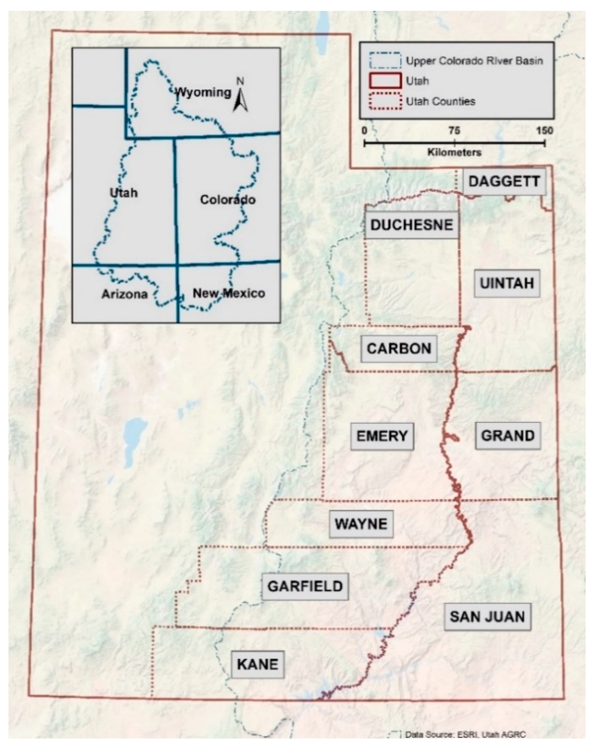
2. Case Study: Colorado River Basin in Utah

The Colorado River serves 40 million people in 7 states of the USA and is one of the most over-allocated rivers in the world. The water availability in the basin is snowmelt driven where about 80% of the precipitation in the basin is in the form of snow. Since the last three decades of the 20th century, the snowmelt has shifted 2–3 weeks earlier [53], which can be linked with the decreased availability of water during the growing season in the basin [54]. Although discrepancies exist among the researchers based on methodological differences, there is a consensus that this region will face a drastic reduction in water supply in the coming decades [55,56,57,58,59,60,61,62,63]. Udall and Overpack estimate a decrease in river flow in the entire basin by up to 20% by mid-century and 35% by the end of this century if business-as-usual warming continues [64].
Agriculture in CRB contributes to about 15% of the total crop production and 13% of livestock in the US [65,66]. 60% of the agricultural land is used to grow forage crops and pasture as feed for cattle [67]. Most of the basin is arid and receives insufficient precipitation, therefore, 90% of cropland is irrigated to supplement the water requirement [67]. In typical farm-ranch operations, calves are born in spring and are a part of the herd for a year. Ranchers raise and feed them on hay that they grow as cattle feed. Cattle are also fed on rangeland and pastures in the summer. Most rangelands are under the Bureau of Land Management or the United States Forest Service that lease the lands to the ranchers yearly. Ranchers round up cattle in the fall and feed the cattle on individual ranches through the winter. They use hay and other supplements to feed the cattle during the season. Young cattle are sold in the spring.
The river is managed by several treaties, regulations, and compacts that are collectively called The Law of the River. The Colorado River Compact (1922) designates Colorado, Wyoming, Utah, Arizona, and New Mexico as part of the Upper Basin [68] (Figure 1). Under the Upper Colorado River Basin Compact of 1948, Utah’s share of water apportioned to the upper basin is 23%. In the Upper Colorado River Basin, river flow has already declined by 16.4% in the last century [69]. Recent trends of earlier-season snowmelt, decreasing snowpack, runoff shifts, and prolonged droughts can be a forerunner to a drier climate [65,70]. The production agriculture–that includes farming, ranching, dairy, and other support industries, is a major economic driver in Utah and contributed $3.5 billion to the state’s economy in 2014 alone [71,72]. As agricultural production is dependent on water availability, climate impacts on agriculture are expected to be severe in the basin. To sustain agriculture in the basin, it is important to understand how climatic variability and other factors affect agricultural production in the region and how the ranchers and farmers adapt to climate-induced changes in production. While many studies have focused on the impact of climate change and variability on water resources in the Colorado River basin, little work has been done on the impacts of changes in climate on agricultural production that we address in the study. Figure 1 shows the 10 counties in the southern and eastern parts of Utah that were chosen for this case study.

3. Methods

This study combines quantitative (statistics and data mining) and qualitative (interview) methods to identify relationships between climate variables (temperature, precipitation, and water availability) and agricultural production (hay production and cattle numbers). The first part of data analysis uses correlation test, multilinear regression, and random forest regression to determine the most important variables that affect cattle and hay production in the study area. In the second part, the first author interviewed farmers in Utah to understand how they have adapted their ranching practices to cope with climate variability in the region and what impacts the changing climate has had on cattle and hay production. The data used in the quantitative analysis has a large variance which the models cannot completely explain. The interviews fill the gap in information that the quantitative analysis cannot describe.

3.1. Statistical Analysis
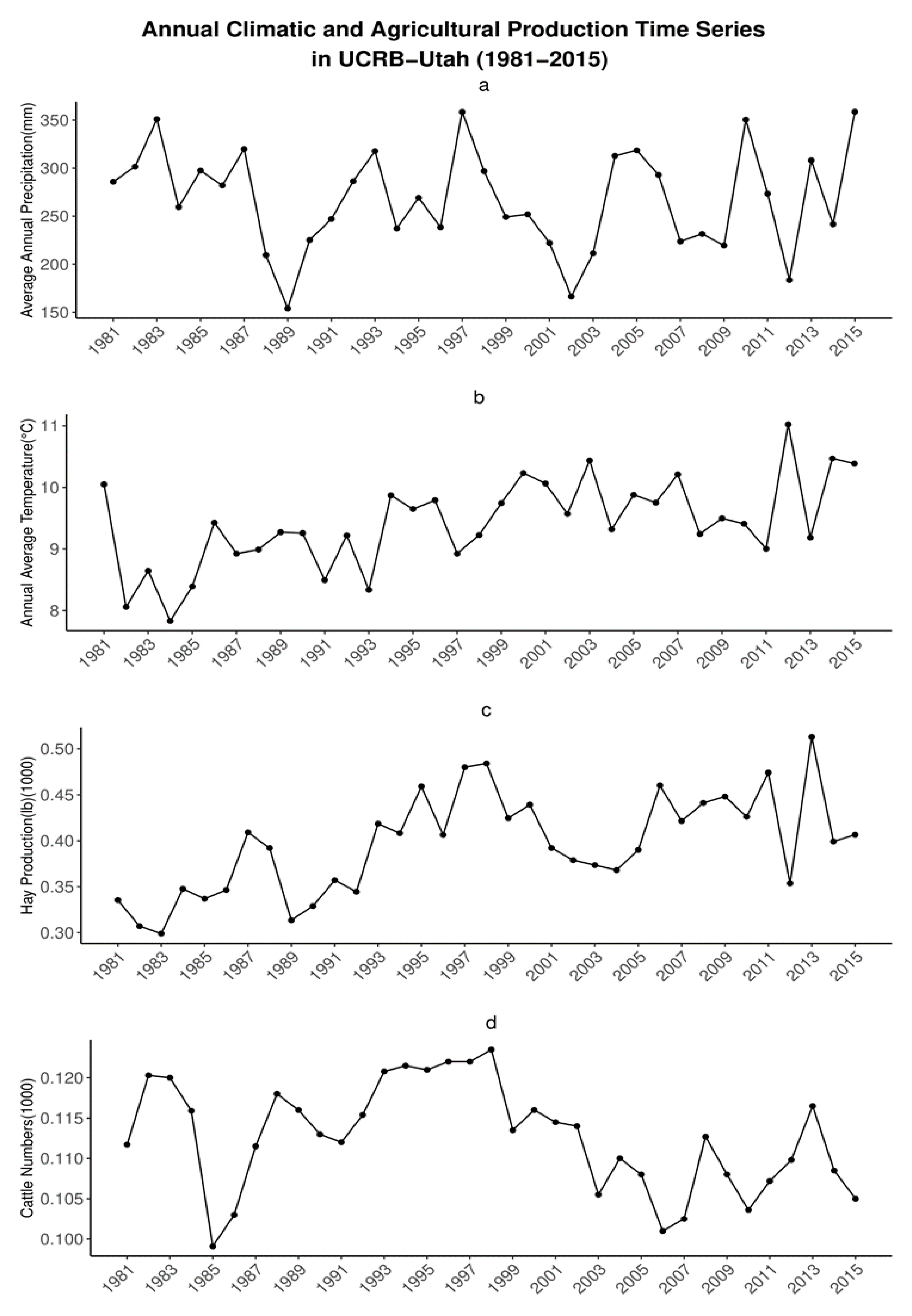
The first part of this study tests the relationships between climatic variables (precipitation and temperature) and agricultural production to identify the variables to which cattle and hay production is most sensitive.

3.1.1. Data

The daily temperature and precipitation data were acquired from the Parameter-elevation Regressions on Independent Slopes Model (PRISM) [73]. Daily data for natural streamflow was downloaded from the Bureau of Reclamation [74]. Natural streamflow is the streamflow that would have existed if there were no reservoir storage on the river and no other consumptive uses were in play. Annual, county-level data for agricultural production (cattle numbers, alfalfa production, alfalfa yield, acres of alfalfa harvested per year) was downloaded from the National Agricultural Statistics Service (NASS) by the US Department of Agriculture [75]. The data were acquired from 1981–2015. A summary of the data, format, and sources is given in Table 1. The data analyses were conducted using R version 3.4.2.

3.1.2. Climate Extreme Indices

The climate extreme indices proposed by the Expert Team on Sector-specific Climate Indices (ET-SCI) are used in the study to test the relation of climate to the hay production and herd size in our study area. The climate indices provide a better characterization of the climate extremes and facilitate in monitoring the trends and intensity of events that might be responsible for the climatic effects on humans and the environment [76]. These indices are derived from daily temperature and precipitation data by calculating the number of days in a year where daily values exceed a set threshold. Before calculating indices, we homogenized the temperature and precipitation time series using penalized maximal t-test and penalized maximal F test [77,78,79,80] in two-step regression. This is done to detect for autocorrelation and inhomogeneities due to non-climatic factors and to adjust the time series accordingly. The homogenization and correction of the daily time series of precipitation and temperature were accomplished using the R-based RHTest_V4 and RHtests_dlyPrcp packages [81,82]. We used these packages because they are the most recent and advanced in the homogenization of series. The Climpact2 software [83] was used to calculate the climate extreme indices from the quality controlled data. The details of the indices used are present in Table S1.
The annual climate extreme indices, natural streamflow data, and agricultural production data for all the counties were aggregated to get one value for each variable per year. Altogether, we used 35 observations of 6 variables in the linear model (Section 3.1.4) whereas we used 35 observations of 22 variables in the random forest model (Section 3.1.5).

3.1.3. Correlation Test

The association between, hay production, cattle herd size, and the climate indices was investigated using correlation test. We used Pearson’s correlation coefficient as a measure of the strength of the relationship between any two variables. For any two indices that had a correlation coefficient greater than |0.5|, the index with a higher correlation with other indices was removed from the data as it did not add any new information to the model and may have created a bias in the result. For example, the indices ‘days with temperature less than 0 °C (txle0)’ and ’icing days’ had a correlation coefficient of 0.99. Icing days have a higher correlation with cattle and hay production and other indices, so txle0 was excluded from further analysis. In the next step, the indices with very low correlation (<0.03) with cattle and hay production were removed.

3.1.4. Multiple Linear Regression

Two data-mining techniques are used to evaluate the relation of climatic parameters to hay production and cattle numbers in the study area. The hypothesized relation of cattle and hay production to climate is tested using multilinear regression (MLR) and random forest regression (RFR).
Multiple linear regression is used to assess whether a relationship exists between the response variables (cattle/hay numbers) and explanatory variables (selected climate indices). MLR is a standard regression technique to study the relation of a response with many predictors where a linear relation is expected between the response and predictors. Since the units of the variables used are different and vary from tens (for temperature) to 100,000 (for cattle numbers), the data were normalized by their standard deviation before implementing MLR. Cattle numbers and hay production (lbs. per year) are response variables whereas the climate indices, streamflow, and acreage of hay are predictors. Since the indices are correlated with each other, they cannot be the predicting variables for MLR. Two indices for precipitation and temperature, that are not correlated to other indices, are chosen as predictor variables.
F statistic value determines the overall significance or fit of the model; the value shows if the group of the predictors are jointly significant. The other parameter to judge the fitness of the model is the p-value of the F statistic, a model with a p-value <0.05 is significant. F statistic and p-value are jointly assessed to evaluate the overall fitness of the model. The individual predictors are evaluated based on the t-statistic value and the variance explained by the predictor in the model. The more the t-statistic value is over zero, the greater is the relative association between the predictor and the response variable.

3.1.5. Random Forest Regression

Random forest regression was chosen as it is superior in predictive ability to other modeling techniques, such as multiple linear regression, artificial neural network, and support vector machine models. It performs well for identifying the most important predictors as well [84,85,86,87,88], especially for variables that have a nonlinear correlation [89]. The Random Forest algorithm is a non-parametric statistical method that uses an ensemble of decision trees where many decision trees are combined into a single model. Each tree is built by breaking-down the data into random subsets that include homogenous responses and only uses data points from that subset to create the tree [90]. The random subsets are created by bootstrap aggregation (bagging) [91]. Bootstrap sets are created by random sampling with replacement. By doing so, each tree uses predictors different from each other. This procedure decorrelates the individual trees, restricts the model from over-fitting the data, and reduces the variance in prediction. Each decision tree is considered a weak learner and individual predictions might not be very accurate. Thus, the predictions of individual trees are aggregated to a single prediction for the model. The predictors in our model are the climate indices for precipitation and temperature, streamflow, hay acreage; cattle and hay production are response variables.
To build the random forest model for our study, we used the randomforest package in R [92]. In the model’s implementation in the randomforest in R, the user has control over two parameters; the number of trees in a forest (ntree) and the number of variables that can be tested on each split (branch) of a tree (mtry). The model identifies and ranks the variables that are most important for the response variable prediction (here cattle numbers and hay production). The percentage of variance explained by the model in randomforest in R represents the best-fit model or forest (R2 value) for ntree and mtry combination. The seed function is used to allow others to reproduce results. Because of our data, changing the values of the three parameters (ntree, mtry, and seed) gives results with high variance and different importance ranking for the indices for each run. To account for this variance, a function was created that uses different combinations of the three parameters from 1:5000. The models that had positive values for R2 were kept and the frequency of occurrence the most important variables were calculated. The indices that occurred as important variables in most of the runs are considered the most important variables for cattle and hay production.

3.2. Qualitative Interview Analysis

Farmers from counties of Utah who irrigate from the Colorado River and its tributaries were interviewed. We contacted the farmers through county extension agents’ recommendations. The interviewees were farmers whose focus on agriculture was cattle production, hay production, or both. They had ranching experience of 15–60 years. Depending on the interviewee’s preference, they were interviewed via phone or sent the questionnaire by email. The phone interviews took almost half an hour each. Interviews were recorded for the participants who gave consent to be recorded
The interview methods were approved by the Utah State University Institutional Review Board (IRB) protocol #10208. Due to difficulty in recruiting and getting farmers to agree to an interview, sign the IRB protocol, and interview at their convenience, nine farmers (eight male, 1 female) participated; 3 from Carbon, 2 from Duchesne and Emery each and 1 from San Juan and Uintah county. In the nine interviews conducted, we started to obtain similar repeated responses. Thus, we refrained from increasing the sample size as we decided that the ranchers/farmers interviewed are representative of other ranchers in the region. The interviewees were asked questions regarding their farming practices, whether they have observed any changes in agricultural production in the last three decades, and what were their adaptation practices to cope with the changes. The complete questionnaire is presented in File S1.
Thematic network analysis [93] was used to analyze the interview data. Similar themes in the responses of ranchers were identified and the responses were grouped in a codebook. The responses were further classified into sub-themes. The codebook was used to analyze the responses and extract meaningful information from the interview data. As participants shared their opinions and perceptions, the authors did not verify these responses.

4. Results

The first part of this section contains results from correlation test, multilinear regression, and random forest regression that aim to identify the important variables for agricultural production. The second part includes results from the qualitative interview to investigate the adaptation practices of the ranchers to the climate variability and other factors in the study area.

4.1. Statistical Analysis

The time series for annual cattle numbers and hay production show that despite the increasing trend in hay production, there is an overall decrease in cattle numbers in the 35 years studied (Figure 2c,d). In some wet years, cattle numbers and hay production are very low and vice versa (Figure 2a,c,d). There is a large variance in cattle numbers and hay produced in the region across wet and dry years. We find lower hay production during the low precipitation years of 1989, 2002, and 2012, whereas in the high precipitation years, hay production was higher in 1997 but lower or normal in 1983, 2010, and 2015. This result suggests that drought affects hay production in UCRB, but not the normal and wet years. Multiple factors including climate and adaptation strategies affect year-to-year variations in hay productions and the number of cattle.

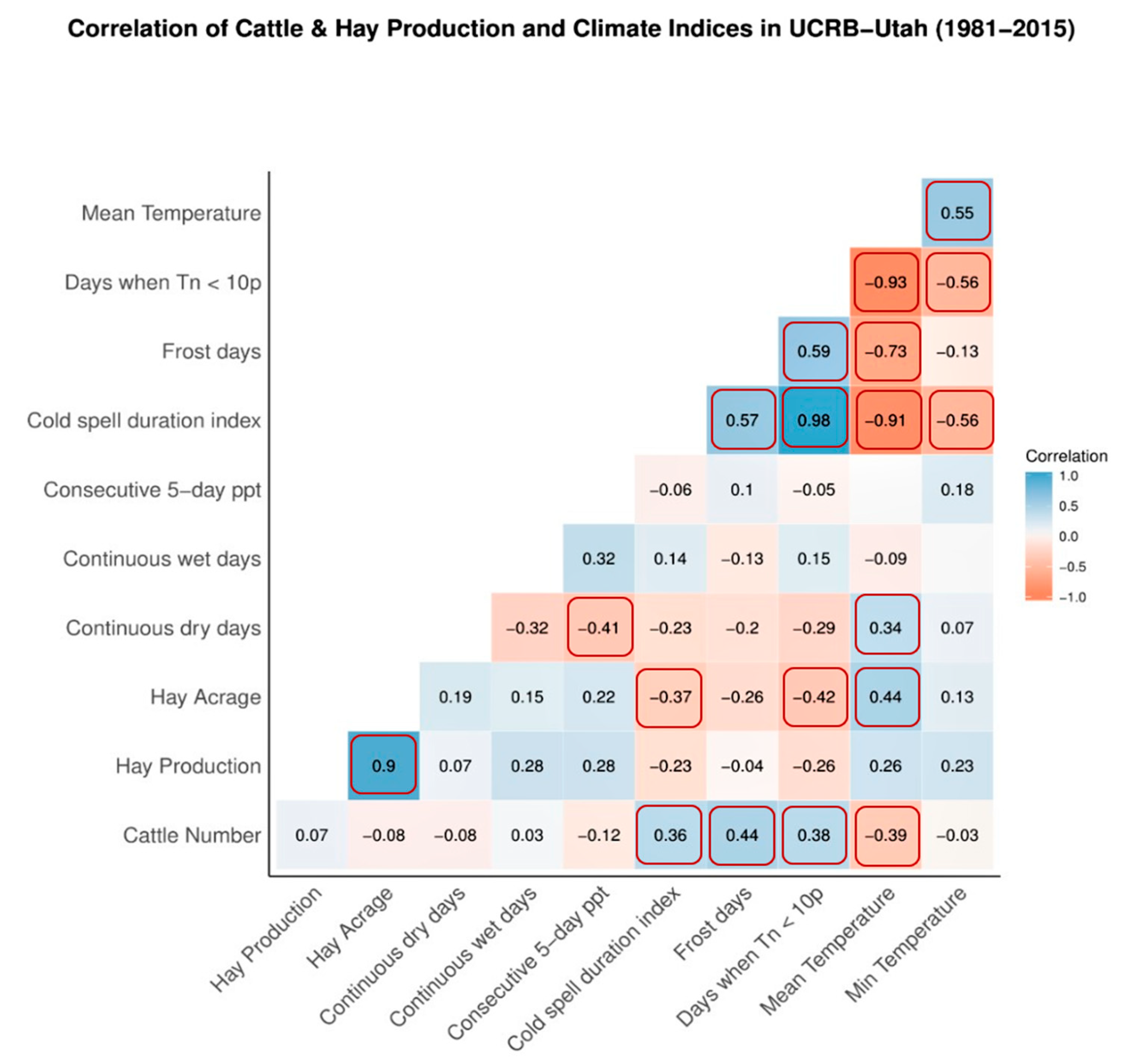
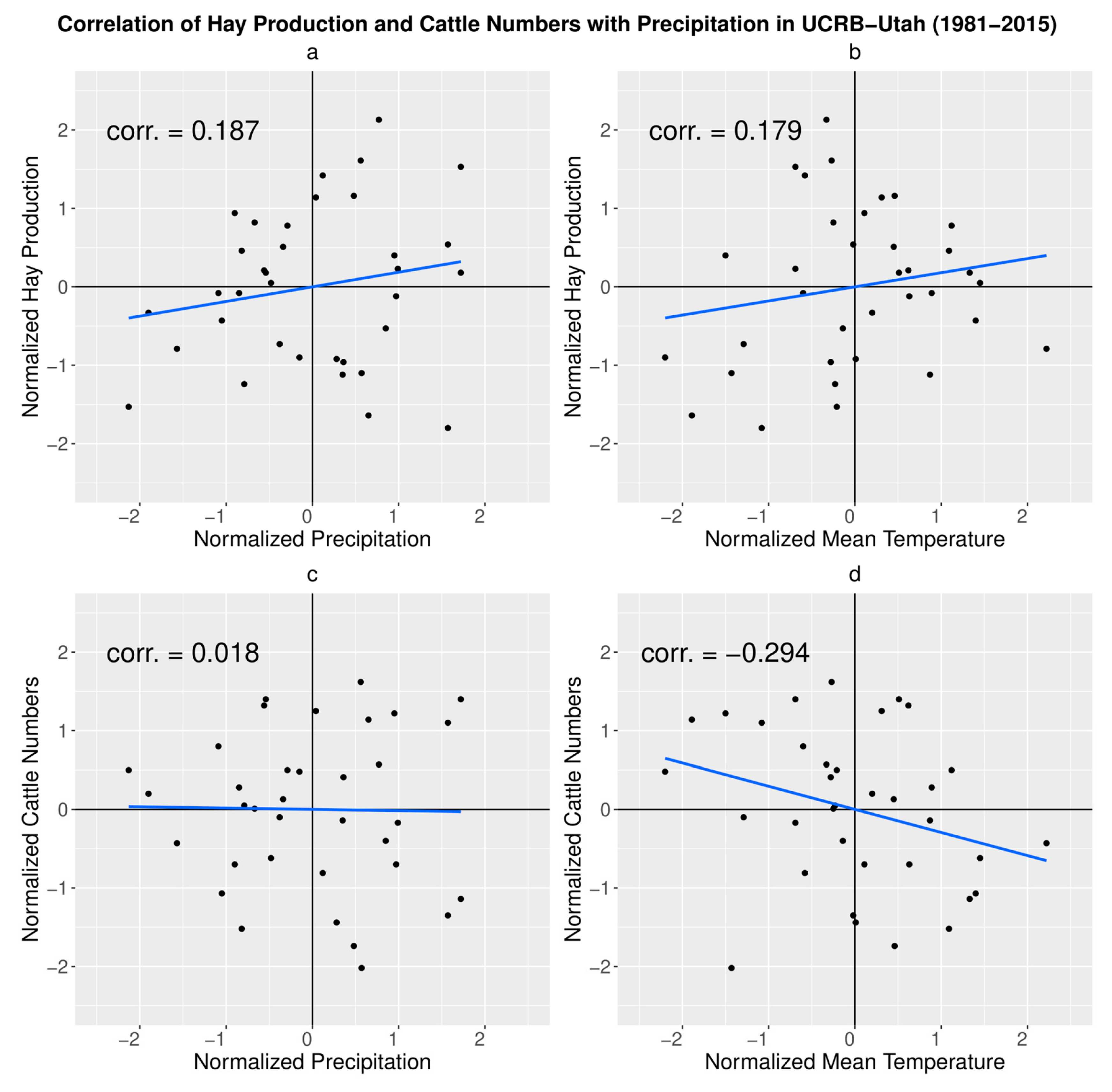
4.1.1. Correlation Test

The results for the Pearson correlation test for the indices and cattle and hay production show that there is a correlation between cattle/ hay production and temperature indices (Figure 3). Statistically significant correlation coefficients (significance level = 0.05) are marked in red. Years with extremely cold temperatures have the strongest positive correlation with cattle numbers, as shown by the correlation coefficient of 0.44 with frost days (Figure 3). The hay production does not correlate significantly with any temperature or precipitation index but merely on the acreage of hay per year (Figure 3). The correlation coefficient value < 0.01 is not shown in the matrix.
Overall, hay production shows a weak linear relation with the precipitation whereas cattle numbers show no relation with changes in precipitation (Figure 4a,c). The mean temperature has a positive linear relation with hay production but a negative linear relation with cattle numbers (Figure 4b,d). Thus, high temperature is favorable for hay production, as it provides a longer growing season. Contrary to that, high temperatures correspond to lower cattle numbers. This may be associated with heat stress-induced mortality in cattle.

4.1.2. Multilinear Regression

The results from the hay model suggest that at least one of the predictor variables is significantly related to hay production, as indicated by the p-value is 6.08e-13 where a value of less than or equal to 0.05 being significant (Table 2). Hay acreage is ranked the most important variable in the hay model as shown by the t-statistic value of 15.019 and 79.74% variance explained (Table 2, Figure 5). This can be explained by the direct relation of the acreage of hay and the overall hay production. Among the climatic indices, none of the variables are significant for hay production as none of them contributes highly to model prediction (Table 2, Figure 5).
The accuracy of the model is determined by the R-squared (R2) value, where the best-fit model has a value near 1. Although the hay model has a better fit for linear regression than the cattle model (Table 2), hay acreage alone explains most of the variance in the model. It can be interpreted as meaning that other indices have minor influence on the number of cattle.
For the cattle model, the p-value of 0.07 implies that there is no significant relationship between climate indices and cattle number/herd size (Table 2). Among the indices used as predictors, frost days are the most important index for cattle herd size as it explains 23.96% of the variance of the model (Figure 6).

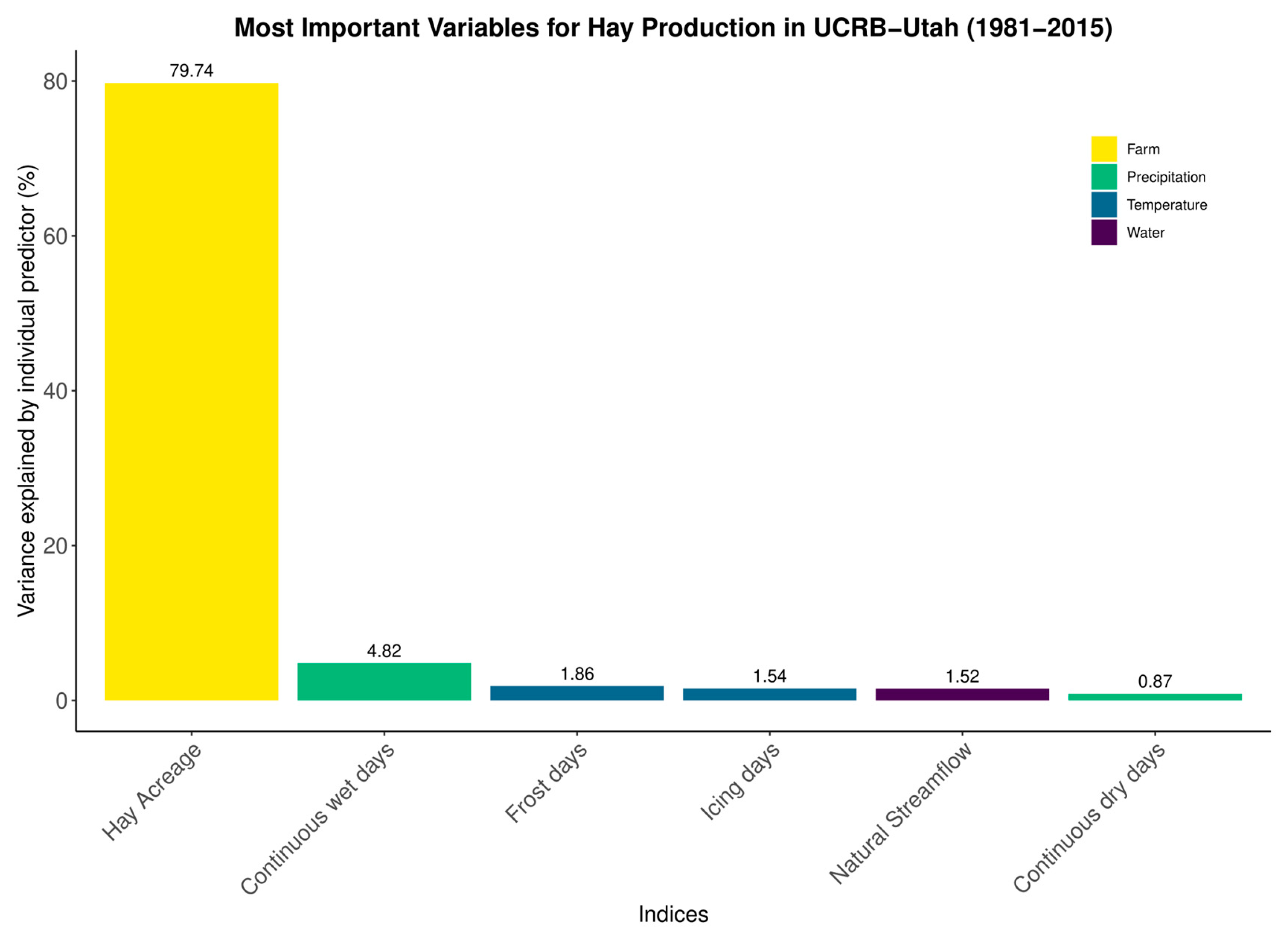
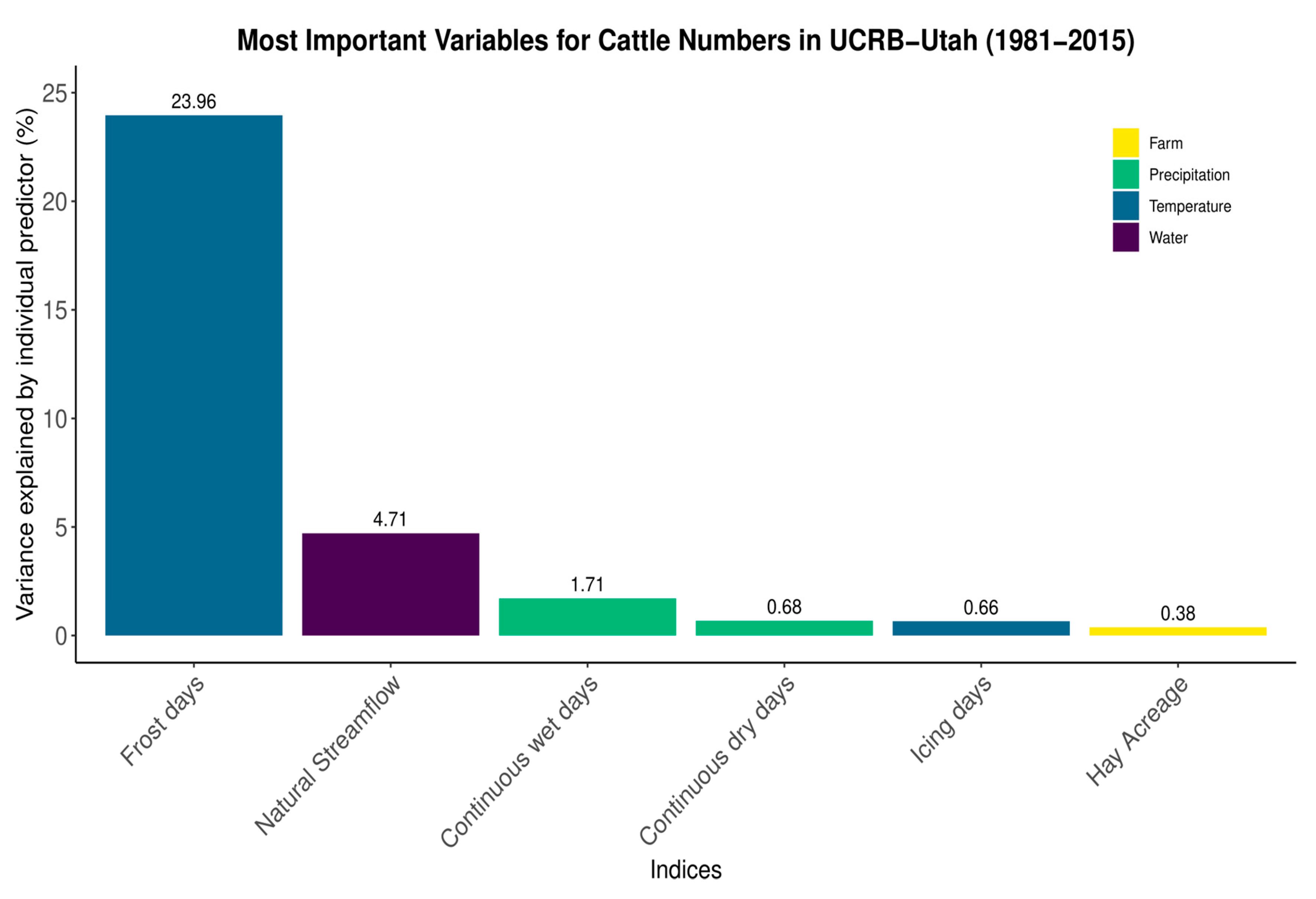
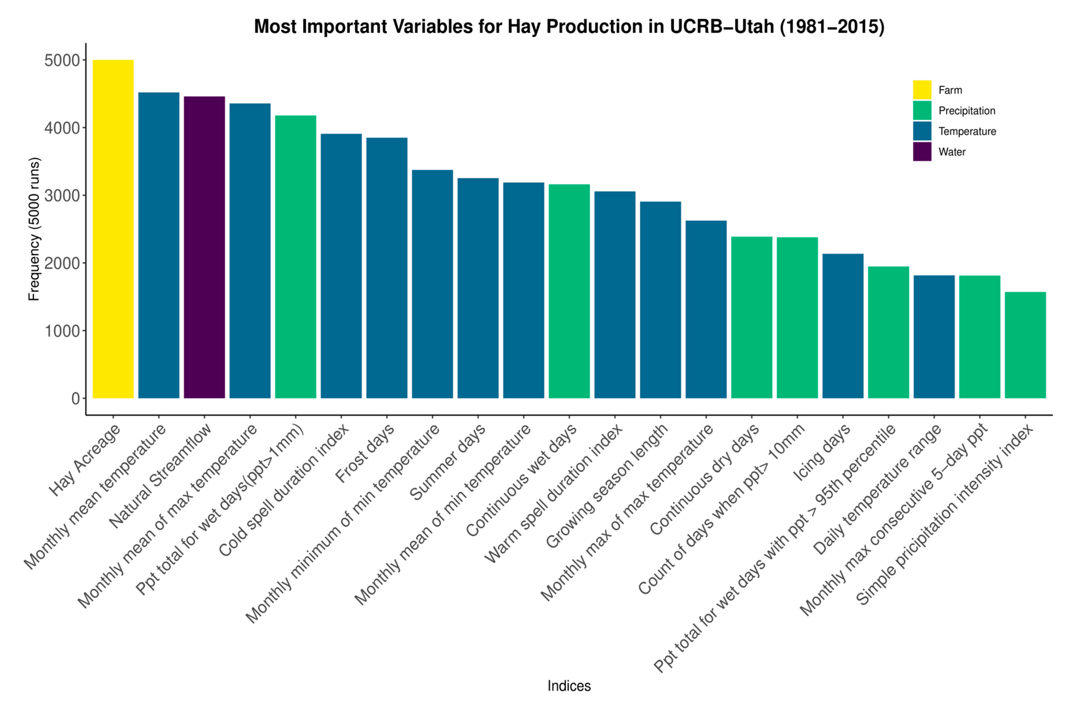
4.1.3. Random Forest Regression

The results from the random forest regression show that climatic variables are more important for hay production than for cattle production as the parameters occur more frequently for the model in hay production than cattle herd numbers (Figure 7 and Figure 8). The index that has the highest frequency of occurrence is considered to have the most influence on herd size or hay production. In the climate indices, the temperature-based indices appear to have more impact on the herd size and hay production in the region (Figure 7 and Figure 8).
Apart from the climatic factors, streamflow (water availability) is an important factor in hay production in the region but is ranked much lower for cattle (Figure 7 and Figure 8). This can be explained by the fact that cattle production is indirectly related to hay (or crop) production, the latter is further related to water availability. The acreage of hay does not appear to be important for cattle herd size (Figure 7 and Figure 8). We explored this aspect in the interviews to identify other factors in play that can influence cattle production and overall herd size.

4.2. Qualitative Interview Analysis

Thematic analysis identified three organizing themes in the data: the effects of climate variability on cattle and hay production, the most important factors that influence cattle and hay production, and the adaptation measures in place and future plans of the farmers (Figure 9).

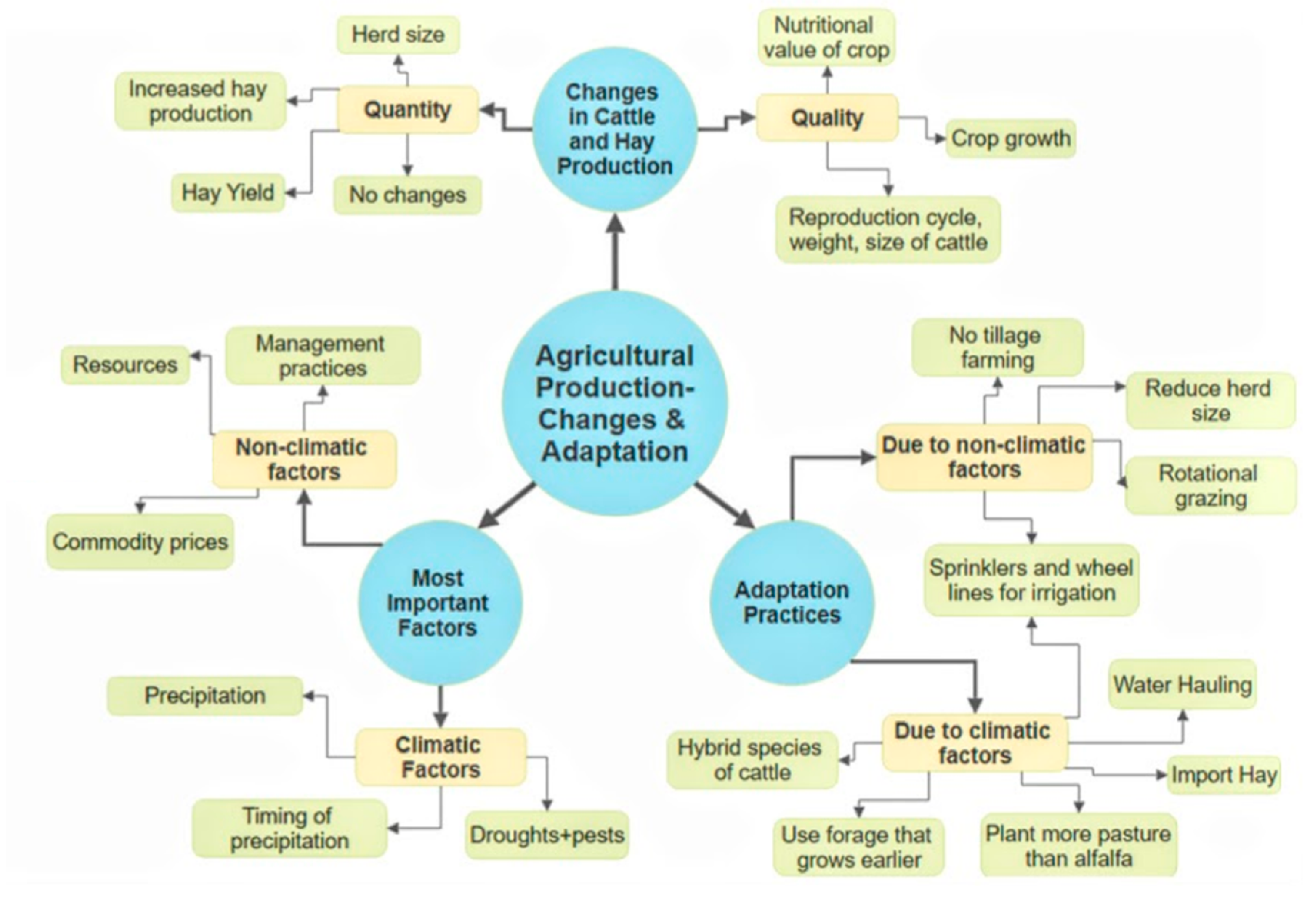
4.2.1. Changes in Cattle and Hay Production

This theme summarizes the responses of the farmers on their observations on changes in cattle and hay production for the last three decades. Most of the interviewed farmers believe that climate variability has unfavorable effects on agricultural production, but it is hard to always narrow down the cause behind hay yield changes in hot and dry weather.
“In some years, the hay doesn’t do as good and I really haven’t narrowed it down if it’s dry or if it’s just hot. It seems like that there are some years when things are so hot that you can’t keep [hay] wet and you have a little bit of drop in yield in those years”.
The quality of forage is directly tied to water availability. With lack of water from heat stress, farmers reported decreased growth of the hay crop. The water-stressed crop is also prone to pest infestation as farmers noted the fact that lack of water reduces plant immunity. In wet years (like 2019), storing hay that has been rained on is difficult. To avoid this, the farmers would delay harvesting the hay. As a result, the crop yield might increase but the nutritional value of the crop would decrease as the crop progresses through the reproductive stage. Only one farmer said that the wet or dry year does not affect the quality of hay but the overall yield (ton/acres) of the crop. A couple of farmers mentioned that they have seen increased crop production on their farms in the last few decades. This increase in production is mainly because of advancements in methods for farming such as automatic moisture sensors, efficient irrigation systems, fertilizers, and mechanization of farms.
The cattle number does not vary a lot in a wet or dry year, but some health-related characteristics change. Sometimes the cows are not pregnant in the fall, then the farmer either must sell the cow or feed them through the winter with no expectation of compensation by selling the calves. The farmers consider this an added burden. Although most farmers reported that they have lighter and weaker animals in their herd on dry years as there is not as much forage available for them, a couple of them noted that the cattle adapt to changes more quickly and there are no significant changes in their herd. A farmer who has been in the ranching business for 30 years in San Juan county mentioned that cattle can become acclimated to climate changes. This means that since these cattle are born to a mother raised on the range, they have adapted to changes. For choosing which animal to keep in the herd, he preferred to keep the cattle that had acclimated to changes in the environment because,
“Multi-generations of cattle that have lived in this landscape have an intuition of the landscape that allows them to adapt to climate change… potentially quicker than the other livestock.”
Farmers believe that although hay production and cattle numbers change from year to year, the overall production in five years or more remains the same. The farmers live from one extreme year to another and, hence, do not see a notable change at the decadal scale. A wet year similar to the water year 2019 (October 2018–September 2019) makes up for the preceding dry years. One farmer noted that changes that occur in the production are normal and inevitable; therefore, they cannot be associated with climate. They believe that these changes have always existed and cannot be linked to climatic shifts.
“I haven’t observed a whole lot of changes in cattle production [over the last 20 years] … I am living from one extreme year to the next. I got a dry year where I reduce herd size and then I got a year like this [2019] that is so wet that I don’t know what to do”.

4.2.2. Most Important Factors

This theme summarizes the responses of farmers where they talk about the most important factors that affect the production on their lands. Most farmers believe that the most important factors in the region for agricultural production are temperature, precipitation, and the timing of precipitation as the weather is “a giant factor” in the production.
The change in yield, apart from climate, is associated with water supply and restriction on the crop a farmer can irrigate in a year. Most farmers get their irrigation water from the nearest reservoir. For some, water availability is not affected a lot in wet or dry years. When asked, they associate this with having a prior water right. Most farmers note that the water availability changes year-to-year, but the water supply has been less than adequate in recent decades. Even though they get part of their water right in dry years, they maintain their business. One farmer said, “We adjust to what is given to us at that time”.
Management practices play a big role in productivity if farmers can innovate. The farmers who have the resources to maintain a private pasture that can be used in dry years can prioritize lands to irrigate based on the water allocation that year. The cattle raised on private land recover quickly from a dry season. If the farmer works on the farm instead of hiring labor, they invest more time and energy into it. Farmers believe that they cannot pay someone enough to care for the crop and cattle the way they do themselves.
Another important part of farm operation noted in the interviews is deciding the herd size. This decision considers commodity prices and overhead costs. Ranchers believe that government regulation of prices does not allow them to obtain a fair price for their cows and calves. However, this statement is not supported by evidence. The biggest drivers of cattle prices are markets based on supply and demand. For example, a farmer with an average-sized ranching operation said,
“If they [the government] need to manipulate [prices], they should do it in a way that farmers can do well and thrive, so it incentivizes more people to be in agriculture … The American government wants people to have cheap food, well that’s fine as long as the American farmers can afford to be successful and make money. But it’s not that way, 95–98% of farmers and ranchers that I know in Utah have to have another job and source of income. In other industries, people can set prices, make money, and do well. It looks like agriculture is left at the bottom of the scale.”
Cattle prices and available forage drive the decision on how many cattle to keep that year.

4.2.3. Adaptation Strategies

The farmers and ranchers mentioned various strategies that they have adopted to sustain their farm operations in response to climate variability and to increase convenience. A rancher with 60 years of experience in Uintah county stated,
“I think every farmer and rancher has their own way of doing things, and every farm is different with different soil conditions, what everyone needs to know what is best for their soil.
A rancher with 70 years of family ranching in three Utah counties, stated,
“We have learned to adapt management and use of certain pastures or permits to compensate for the type of condition we have to deal with. This is on a yearly basis or even a semi-year issue. “
The most quoted practice that has changed over time was using sprinklers and rolling (wheel) lines for irrigation instead of flood irrigation. This shift is due to limited water availability, and due to increased efficiency and convenience of modern irrigation systems.
“The only real change that I have noticed is that I have moved from flood irrigation to sprinkler, and part of that is just to be more efficient with water, and part of it is just for convenience… it was a lot more work to irrigate with ditches; with pivots, you hit a button and they are watering”.
Ranchers also mentioned hauling water for livestock and buying hay to use as feed as strategies to handle a shortage of water in dry years. Other practices mentioned in the interviews to preserve land and improve pastures are no-tillage operations and rotational grazing.
To maintain cattle, farmers plant more pasture than alfalfa, so they can bring the cattle to the range earlier. Likewise, they are looking into using grain or forage that starts growing earlier. For those who have the resources, they keep the cow on a farm in a dry year and supplement the feed from other sources. In dry years, some farmers keep part of their herd on the private pastures and not on the Bureau of Land Management (BLM) grazing lands.
“I have a big block of private ground that is rangeland … on bad years, I have to use that but on good years I don’t. So that just sits there and grows, gets healthy and recovers in the years when I don’t have to use it. On dry years when I can’t put my cows on the BLM ranges, I have got a private range to fall back on, I can feed on it, I can haul hay out there and supplement on it without worrying about any federal regulations about not doing it on BLM land. Having a private range has been a real help that I can use or not use depending on my needs.”
This strategy is only viable for the farmers with bigger lands and private pastures where they can keep the cattle for at least a season without jeopardizing their health. As a farmer noted,
“On drier years, my farm is a lot less productive and on wetter years when I have water, I can grow more hay than I need… On years when it’s dry, I am using hay early, I am running out of grazing. The last few years I have to keep my cows off the spring range and feed them. That hurts when you can’t take them to spring range, feeding them 90 or 100 days longer than you expected to, that’s tough!”.
Most farmers reduce herd size on dry years but do so as a last resort. They note that they need to bring the cattle earlier to the rangeland due to the lack of availability of forage. Also, they must keep fewer cattle in their herd on a dry year. A farmer with a big ranch in San Juan County noted that he is experimenting with native cattle to get a hybrid breed with the Criollo cow as it is more adaptable to an arid environment. The hybrid breed is expected to be smaller, travel longer distance for water, use a wider variety of forage and would be more resilient to temperature (than the cattle that has acclimated to climate) too; but it will take at least a decade to find out whether the hybrid was a success for the Southern Utah landscape and climatic conditions or not.

5. Discussion

When identifying the relationship between climate and agricultural production, the correlation test found that the climatic parameters and indices tested had correlation coefficient values less than 0.5. Temperature indices had a statistically significant correlation with cattle numbers whereas hay production did not correlate to the indices used in the study. Using indices as indicators of temperature and precipitation, this result implies that temperature has more impact on cattle and hay production than precipitation. This result is contrary to what was expected and what is presented in previous studies where climatic parameters (temperature and precipitation) have shown a significant relationship on the cattle and crop production [5,6,27,29,33,35,36].
The results from the correlation test and linear regression show that climate indices and cattle and hay production do not have a linear relation. Random forest allows us to test the non-linear relationship between the variables by dividing the dataset into smaller sub-spaces. The results from the random forest regression show that climatic parameters are more important for hay production than cattle herd size as the frequency of occurrence of the indices in importance ranking is more for hay production than for cattle number (Figure 8 and Figure 9). In the climate indices, the temperature-based indices appear to have more impact on the cattle and hay production in the region than precipitation-based indices (Figure 8 and Figure 9). As the crops are irrigated and water supplied through storage, precipitation does not directly affect the crop production and cattle numbers. The results rank streamflow (water availability) high as an important factor in hay production. These results are in parallel to the results of previous studies in terms of ongoing post millennium drought; changes in temperature have a more pronounced effect on river flows (hence water availability) [64,69]. It implies that temperature changes drive streamflow and by extension the crop production in the region. Streamflow is ranked much lower for cattle, which can be explained by the fact that herd size does not necessarily relate to water availability but on other driving factors as learned from the interviews. The acreage of hay does not appear to be important for cattle herd size (Figure 8 and Figure 9). We explore this aspect in the interviews to identify other factors at play that can influence cattle production and the farmers’ decision to maintain the number of cattle in the herd every year. We hypothesized that climatic parameters influence hay and cattle production. Such an impact can be considered minor as per the quantitative analysis, as very few indices have a statistically significant correlation with cattle numbers and hay production. The quantitative analysis does not show a distinct pattern or relationship between climate and agriculture on the annual time scale. There is largely a consensus among farmers that year-to-year variability in temperature and precipitation harms the cattle and hay production. Many adaptation techniques were mentioned in the interviews that included changing irrigation practices and cropping patterns to produce enough forage for the cattle to maintain the number of cattle on the ranches, experimenting to produce hybrid species of cattle, that are resilient to hotter temperature and can use a wider variety of forage. Not all of these adaptation measures have been adopted as a response to climate, but some were adopted to increase convenience and reduce labor costs. Some farmers consider the changes in climate as normal, similar to what Liu et. al found in their study about perceptions of Nevada farmers on climate [94]. Other prior studies also show that non-climatic factors such as lack of resources, limited market access, [45], local market availability, market prices [40], social factors such as social history, and the social nature of risk management [41,95] can be the driving force behind the adaptation and changes in practices for farmers. Although local prices of cattle are generally driven by the global market, they have a strong impact on the local economy. In the UCRB in Utah, cattle prices can be a big factor affecting farmers’ decision to decide on the herd size and the crop to plant year by year.

Limitations

The main limitation of this study was data availability. The only source of agricultural data was from NASS, which reports the data yearly. We could not identify the time of year at which the NASS surveys are made. Thus, the data might be missing for parts of the year and the available data may not account for an entire year. The data sets that we could use for all 10 counties of Utah in the study were only available for cattle numbers and alfalfa production. Thus, we could not identify how much of the change in hay production or cattle numbers was due to irrigation or other technology improvements. The unpredictability of the random forest model is very high, thus we ran the same model 5000 times to account for the variability in results. More variables that can account for the economic aspect of agricultural production can be included to bridge the gap. For larger datasets, deep-learning methods such as deep neural networks can be used in future studies to investigate the similar relationship between climate variables and agricultural production in future studies.
The impact of the commodity prices on a farmer’s decision to keep a herd size to a limit should be accounted for as it plays an important role in farm operations. This can be done using more sophisticated agronomic/economic models. Most farmers and ranchers are mindful of the climate impact on agriculture, but a few can adapt to the changes in climate to maintain the same profitability. The individual adaptive capacity of a farmer depends on many social and economic factors.

6. Conclusions

Agriculture is a sector extremely vulnerable to changes in climate. The warming trends show that there will be less water available in the Colorado River Basin. While many prior studies have identified the effects of changing climate on temperature, precipitation, and streamflow, it is important to describe how climate will and has affected agricultural practices and how farmers/ranchers have been and will continue to adapt to the changes. This study identified the different variables that influence agricultural production and how the ranchers in the Upper Colorado River Basin in Utah have been adapting to those changes. It was hypothesized that variability in climate has a direct impact on cattle and hay production in Utah regions of UCRB. This study used a mixed-method approach in which the relationship between climate and agriculture is investigated using quantitative and qualitative analyses.
The quantitative results did not identify any strong correlation, trends, or influence between the temperature, precipitation, or water availability indices and cattle and hay production. In the weak correlation found, temperature has more influence on cattle and hay production than precipitation. Non-climatic factors have more influence on agricultural production in the study area than the climatic parameters studied. The qualitative interviews allowed deeper exploration of climate–agriculture relationships. For example, we learned that farmers perceive changes in hay and cattle production over time in response to a changing climate. The most important factors are precipitation and timing of precipitation. The farmers are already adapting by switching to sprinkler and wheel irrigation systems, planting more pasture than alfalfa to bring cattle to pastures earlier, and reducing herd size as a last resort. Our work highlights that farmers are well aware of climate changes and are already adapting their practices to maintain hay and cattle productivity on their farms.

Supplementary Materials

The following are available online at https://www.mdpi.com/2225-1154/8/9/96/s1, Table S1: List of Climate Indices, File S1: Questionnaire for Interviews.

Author Contributions

Conceptualization, H.A., L.N.A., D.E.R., Y.C.; methodology, H.A., L.N.A., D.E.R., Y.C.; data collection (interviews), H.A; formal analysis, H.A.; writing—original draft preparation, H.A.; writing—review and editing, H.A., L.N.A., D.E.R., Y.C.; visualization, H.A.; supervision, L.N.A., D.E.R., Y.C.; All authors have read and agreed to the published version of the manuscript.

Funding

This research was funded by Fulbright and Utah Water Research Lab, Logan UT USA.Y.C. was supported by the Utah Agricultural Experiment Station, Utah State University (approved as journal paper number 9380), and the U.S. Department of Interior, Bureau of Reclamation (R18AC00018, R19AP00149).

Acknowledgments

We thank Emily Wilkins (Utah State University) for reproducing the results of this study.

Conflicts of Interest

The authors declare no conflict of interest.

Data Availability and Reproducibility Statement

The data and code for the figures in the quantitative analysis can be accessed at the Hydroshare repository [96]. The data for the interviews cannot be made available because of restrictions imposed by the USU Institutional Research Board that approved the interviews with farmers [97]. Emily Wilkins (Utah State University) downloaded and ran the R scripts and reproduced the results in the figures in the quantitative section of this study.

References

  1. Adams, R.M.; Hurd, B.H.; Lenhart, S.; Leary, N. Effects of global climate change on agriculture: An interpretative review. Clim. Res. 1998, 11, 19–30. [Google Scholar] [CrossRef] [Green Version]
  2. Hoffmann, U. Section B: Agriculture: A key driver and a major victim of global warming. In Key Development Challenges of a Fundamental Transformation of Agriculture; Trade and Environment Review; United Nations Conference on Trade and Development (UNCTAD): Geneva, Switzerland, 2013; pp. 3–5. [Google Scholar]
  3. Yohannes, H. A Review on Relationship between Climate Change and Agriculture. J. Earth Sci. Clim. Chang. 2015, 7. [Google Scholar] [CrossRef]
  4. Ray, D.K.; West, P.C.; Clark, M.; Prischepov, A.V.; Chatterjee, S. Climate change has likely already affected global food production. PLoS ONE 2019, 14. [Google Scholar] [CrossRef]
  5. Ray, D.K.; Gerber, J.S.; Macdonald, G.K.; West, P.C. Climate variation explains a third of global crop yield variability. Nat. Commun. 2015, 6, 1–9. [Google Scholar] [CrossRef] [Green Version]
  6. Vogel, E.; Donat, M.G.; Alexander, L.V.; Meinshausen, M.; Ray, D.K.; Karoly, D.; Meinshausen, N.; Frieler, K. The effects of climate extremes on global agricultural yields. Environ. Res. Lett. 2019, 14, 054010. [Google Scholar] [CrossRef]
  7. Bird, D.N.; Benabdallah, S.; Gouda, N.; Hummel, F.; Koeberl, J.; La Jeunesse, I.; Meyer, S.; Prettenthaler, F.; Soddu, A.; Woess-Gallasch, S. Modelling climate change impacts on and adaptation strategies for agriculture in Sardinia and Tunisia using AquaCrop and value-at-risk. Sci. Total Environ. 2016, 543, 1019–1027. [Google Scholar] [CrossRef] [PubMed]
  8. Lehmann, N. Regional Crop Modeling: How Future Climate May Impact Crop Yields in Switzerland. YSA 2011, 4, 269–291. [Google Scholar]
  9. Birthal, P.S.; Khan, M.T.; Negi, D.S.; Agarwal, S. Impact of Climate Change on Yields of Major Food Crops in India: Implications for Food Security. Agric. Econ. Res. Rev. 2014, 27, 145–155. [Google Scholar] [CrossRef]
  10. Bhattarai, M.D.; Secchi, S.; Schoof, J. Projecting corn and soybeans yields under climate change in a Corn Belt watershed. Agric. Syst. 2017, 152, 90–99. [Google Scholar] [CrossRef] [Green Version]
  11. Schlenker, W.; Roberts, M.J. Estimating the Impact of Climate Change on Crop Yields: The importance of nonlinear temperature effects. NBER Work. Pap. 2008. [Google Scholar] [CrossRef]
  12. Kang, Y.; Khan, S.; Ma, X. Climate change impacts on crop yield, crop water productivity and food security—A review. Prog. Nat. Sci. 2009, 19, 1665–1674. [Google Scholar] [CrossRef]
  13. Salvo, D. Measuring the effect of climate change on agriculture: A literature review of analytical models. J. Dev. Agric. Econ. 2013, 5, 499–509. [Google Scholar] [CrossRef] [Green Version]
  14. Soler, C.M.T.; Sentelhas, P.C.; Hoogenboom, G. Application of the CSM-CERES-Maize model for planting date evaluation and yield forecasting for maize grown off-season in a subtropical environment. Eur. J. Agron. 2007, 27, 165–177. [Google Scholar] [CrossRef]
  15. Walker, N.J.; Schulze, R.E. An assessment of sustainable maize production under different management and climate scenarios for smallholder agro-ecosystems in KwaZulu-Natal, South Africa. Phys. Chem. Earth Parts ABC 2006, 31, 995–1002. [Google Scholar] [CrossRef]
  16. Yao, F.; Xu, Y.; Lin, E.; Yokozawa, M.; Zhang, J. Assessing the impacts of climate change on rice yields in the main rice areas of China. Clim. Chang. 2007, 80, 395–409. [Google Scholar] [CrossRef]
  17. Dhungana, P.; Eskridge, K.M.; Weiss, A.; Baenziger, P.S. Designing crop technology for a future climate: An example using response surface methodology and the CERES-Wheat model. Agric. Syst. 2006, 87, 63–79. [Google Scholar] [CrossRef]
  18. Eitzinger, J.; Štastná, M.; Žalud, Z.; Dubrovský, M. A simulation study of the effect of soil water balance and water stress on winter wheat production under different climate change scenarios. Agric. Water Manag. 2003, 61, 195–217. [Google Scholar] [CrossRef]
  19. Luo, Q.; Williams, M.A.J.; Bellotti, W.; Bryan, B. Quantitative and visual assessments of climate change impacts on South Australian wheat production. Agric. Syst. 2003, 77, 173–186. [Google Scholar] [CrossRef]
  20. Krishnan, P.; Swain, D.K.; Chandra Bhaskar, B.; Nayak, S.K.; Dash, R.N. Impact of elevated CO2 and temperature on rice yield and methods of adaptation as evaluated by crop simulation studies. Agric. Ecosyst. Environ. 2007, 122, 233–242. [Google Scholar] [CrossRef]
  21. Anwar, M.R.; O’Leary, G.; McNeil, D.; Hossain, H.; Nelson, R. Climate change impact on rainfed wheat in south-eastern Australia. Field Crops Res. 2007, 104, 139–147. [Google Scholar] [CrossRef]
  22. Hua, X.; Eheart, J. Wayland Assessing Vulnerability of Water Resources to Climate Change in Midwest. In Proceedings of the World Water and Environmental Resources Congress 2003, Philadelphia, PA, USA, 23–26 June 2003; pp. 1–10. [Google Scholar] [CrossRef]
  23. Steduto, P.; Hsiao, T.C.; Raes, D.; Fereres, E. AquaCrop-The FAO Crop Model to Simulate Yield Response to Water: I. Concepts and Underlying Principles. Agron. J. 2009, 101, 426–437. [Google Scholar] [CrossRef] [Green Version]
  24. Kikoyo, D.A.; Nobert, J. Assessment of impact of climate change and adaptation strategies on maize production in Uganda. Phys. Chem. Earth 2016, 93, 37–45. [Google Scholar] [CrossRef]
  25. Schauberger, B.; Archontoulis, S.; Arneth, A.; Balkovic, J.; Ciais, P.; Deryng, D.; Elliott, J.; Folberth, C.; Khabarov, N.; Müller, C.; et al. Consistent negative response of US crops to high temperatures in observations and crop models. Nat. Commun. 2017, 8, 13931. [Google Scholar] [CrossRef] [PubMed] [Green Version]
  26. Chenu, K.; Porter, J.R.; Martre, P.; Basso, B.; Chapman, S.C.; Ewert, F.; Bindi, M.; Asseng, S. Contribution of Crop Models to Adaptation in Wheat. Trends Plant Sci. 2017, 22, 472–490. [Google Scholar] [CrossRef]
  27. Crescio, M.I.; Forastiere, F.; Maurella, C.; Ingravalle, F.; Ru, G. Heat-related mortality in dairy cattle: A case crossover study. Prev. Vet. Med. 2010, 97, 191–197. [Google Scholar] [CrossRef]
  28. Hansen, P.J. Effects of heat stress on mammalian reproduction. Philos. Trans. R. Soc. B Biol. Sci. 2009, 364, 3341–3350. [Google Scholar] [CrossRef]
  29. Nardone, A.; Ronchi, B.; Lacetera, N.; Ranieri, M.S.; Bernabucci, U. Effects of climate changes on animal production and sustainability of livestock systems. Livest. Sci. 2010, 130, 57–69. [Google Scholar] [CrossRef]
  30. Key, N.; Sneeringer, S. Potential effects of climate change on the productivity of U.S. dairies. Am. J. Agric. Econ. 2014, 96, 1136–1156. [Google Scholar] [CrossRef]
  31. St-Pierre, N.R.; Cobanov, B.; Schnitkey, G. Economic Losses from Heat Stress by US Livestock Industries. J. Dairy Sci. 2003, 86, E52–E77. [Google Scholar] [CrossRef] [Green Version]
  32. Craine, J.M.; Elmore, A.J.; Olson, K.C.; Tolleson, D. Climate change and cattle nutritional stress. Glob. Chang. Biol. 2010, 16, 2901–2911. [Google Scholar] [CrossRef]
  33. Henry, B.; Charmley, E.; Eckard, R.; Gaughan, J.B.; Hegarty, R. Livestock production in a changing climate: Adaptation and mitigation research in Australia. Crop Pasture Sci. 2012, 63, 191–202. [Google Scholar] [CrossRef]
  34. Polley, H.W.; Briske, D.D.; Morgan, J.A.; Wolter, K.; Bailey, D.W.; Brown, J.R. Climate change and North American rangelands: Trends, projections, and implications. Rangel. Ecol. Manag. 2013, 66, 493–511. [Google Scholar] [CrossRef]
  35. Reeves, M.C.; Bagne, K.E. Vulnerability of Cattle Production to Climate Change on U.S. Rangelands; US Department of Agriculture, Forest Service, Rocky Mountain Research Station: Fort Collins, CO, USA, 2016; Volume 39, p. 343. [Google Scholar]
  36. Rust, J.; Rust, T. Climate change and livestock production: A review with emphasis on Africa. S. Afr. J. Anim. Sci. 2013, 43, 255. [Google Scholar] [CrossRef] [Green Version]
  37. Rojas-Downing, M.M.; Nejadhashemi, A.P.; Harrigan, T.; Woznicki, S.A. Climate change and livestock: Impacts, adaptation, and mitigation. Clim. Risk Manag. 2017, 16, 145–163. [Google Scholar] [CrossRef]
  38. Abid, M.; Schilling, J.; Scheffran, J.; Zulfiqar, F. Climate change vulnerability, adaptation and risk perceptions at farm level in Punjab, Pakistan. Sci. Total Environ. 2016, 547, 447–460. [Google Scholar] [CrossRef] [PubMed]
  39. Arendse, A.; Crane, T.A. Impacts of climate change on smallholder farmers in Africa and their adaptation strategies: What are the roles for research. In Proceedings of the International Symposium and Consultation, Arusha, Tanzania, 29–31 March 2010. [Google Scholar]
  40. Bhatta, G.D.; Aggarwal, P.K.; Kristjanson, P.; Shrivastava, A.K. Climatic and non-climatic factors influencing changing agricultural practices across different rainfall regimes in South Asia. Curr. Sci. 2016, 110, 1272–1281. [Google Scholar] [CrossRef]
  41. Crane, T.A.; Roncoli, C.; Hoogenboom, G. Adaptation to climate change and climate variability: The importance of understanding agriculture as performance. NJAS Wagening. J. Life Sci. 2011, 57, 179–185. [Google Scholar] [CrossRef] [Green Version]
  42. Li, X.; Takahashi, T.; Suzuki, N.; Kaiser, H.M. The impact of climate change on maize yields in the United States and China. Agric. Syst. 2011, 104, 348–353. [Google Scholar] [CrossRef]
  43. Sandve, G.K.; Nekrutenko, A.; Taylor, J.; Hovig, E. Ten Simple Rules for Reproducible Computational Research. PLoS Comput. Biol. 2013, 9, 1–4. [Google Scholar] [CrossRef] [Green Version]
  44. Smit, B.; Skinner, M.W. Adaptation options in agriculture to climate change: A typology. Mitig. Adapt. Strateg. Glob. Chang. 2002, 7, 85–114. [Google Scholar] [CrossRef]
  45. Uddin, M.N.; Bokelmann, W.; Entsminger, J.S. Factors Affecting Farmers’ Adaptation Strategies to Environmental Degradation and Climate Change Effects: A Farm Level Study in Bangladesh. Climate 2014, 2, 223–241. [Google Scholar] [CrossRef] [Green Version]
  46. Richards, P. Cultivation: Knowledge or performance. In An Anthropological Critique of Development: The Growth of Ignorance; Routledge: Abingdon-on-Thames, UK, 1993; pp. 61–78. [Google Scholar]
  47. Mendelsohn, R.; Dinar, A. Climate change, agriculture, and developing countries: Does adaptation matter? World Bank Res. Obs. 1999, 14, 277–293. [Google Scholar] [CrossRef] [Green Version]
  48. McCarthy, N.; Lipper, L.; Branca, G. Climate-Smart Agriculture: Smallholder Adoption and Implications for Climate Change Adaptation and Mitigation. Mitig. Clim. Chang. Agric. Work. Pap. 2011, 3, 1–37. [Google Scholar]
  49. Colloff, M.J.; Martín-López, B.; Lavorel, S.; Locatelli, B.; Gorddard, R.; Longaretti, P.Y.; Walters, G.; van Kerkhoff, L.; Wyborn, C.; Coreau, A.; et al. An integrative research framework for enabling transformative adaptation. Environ. Sci. Policy 2017, 68, 87–96. [Google Scholar] [CrossRef]
  50. Rickards, L.; Howden, S.M. Transformational adaptation: Agriculture and climate change. Crop Pasture Sci. 2012, 63, 240–250. [Google Scholar] [CrossRef]
  51. Rippke, U.; Ramirez-Villegas, J.; Jarvis, A.; Vermeulen, S.J.; Parker, L.; Mer, F.; Diekkrüger, B.; Challinor, A.J.; Howden, M. Timescales of transformational climate change adaptation in sub-Saharan African agriculture. Nat. Clim. Chang. 2016, 6, 605. [Google Scholar] [CrossRef]
  52. Howden, S.M.; Soussana, J.-F.J.-F.; Tubiello, F.N.; Chhetri, N.; Dunlop, M.; Meinke, H. Adapting agriculture to climate change. Proc. Natl. Acad. Sci. USA 2007, 104, 19691. [Google Scholar] [CrossRef] [Green Version]
  53. Clow, D.W. Changes in the timing of snowmelt and streamflow in Colorado: A response to recent warming. J. Clim. 2010, 23, 2293–2306. [Google Scholar] [CrossRef]
  54. Das, T.; Pierce, D.W.; Cayan, D.R.; Vano, J.A.; Lettenmaier, D.P. The importance of warm season warming to western U.S. streamflow changes. Geophys. Res. Lett. 2011, 38, 1–5. [Google Scholar] [CrossRef] [Green Version]
  55. Cayan, D.R.; Das, T.; Pierce, D.W.; Barnett, T.P.; Tyree, M.; Gershunov, A. Future dryness in the southwest US and the hydrology of the early 21st century drought. Proc. Natl. Acad. Sci. USA 2010, 107, 21271–21276. [Google Scholar] [CrossRef] [Green Version]
  56. Hamlet, A.F.; Mote, P.W.; Clark, M.P.; Lettenmaier, D.P. Twentieth-century trends in runoff, evapotranspiration, and soil moisture in the western United States. J. Clim. 2007, 20, 1468–1486. [Google Scholar] [CrossRef] [Green Version]
  57. Dawadi, S.; Ahmad, S. Changing climatic conditions in the Colorado River Basin: Implications for water resources management. J. Hydrol. 2012, 430–431, 127–141. [Google Scholar] [CrossRef]
  58. Wehner, M.F.; Arnold, J.R.; Knutson, T.; Kunkel, K.E.; LeGrande, A.N. Droughts, floods, and wildfires. In Climate Science Special Report: Fourth National Climate Assessment; Wuebbles, D.J., Fahey, D.W., Hibbard, K.A., Dokken, D.J., Stewart, B.C., Maycock, T.K., Eds.; CreateSpace Independent Publishing Platform: Scotts Valley, CA, USA, 2017; pp. 231–256. [Google Scholar]
  59. Hoerling, M.; Jon, E. Past Peak Water in Southweast. Southwest Hydrol. 2007, 6, 18–19. [Google Scholar]
  60. McCabe, G.J.; Wolock, D.M. Warming may create substantial water supply shortages in the Colorado River basin. Geophys. Res. Lett. 2007, 34, 1–5. [Google Scholar] [CrossRef] [Green Version]
  61. McMurrray, C. The Colorado River Basin and Climate: Perfect Storm for the Twenty-First Century. Available online: https://www.coloradocollege.edu/dotAsset/74e91de4-a1ff-4062-b628-030e997b4e0b.pdf (accessed on 20 April 2018).
  62. Vano, J.A.; Das, T.; Lettenmaier, D.P. Hydrologic Sensitivities of Colorado River Runoff to Changes in Precipitation and Temperature *. J. Hydrometeorol. 2012, 13, 932–949. [Google Scholar] [CrossRef] [Green Version]
  63. Christensen, N.; Lettenmaier, D.P. A multimodel ensemble approach to assessment of climate change impacts on the hydrology and water resources of the Colorado River Basin. Hydrol. Earth Syst. Sci. 2007, 3, 3727–3770. [Google Scholar] [CrossRef] [Green Version]
  64. Udall, B.; Overpeck, J. The twenty-first century Colorado River hot drought and implications for the future. Water Resour. Res. 2017, 53, 2404–2418. [Google Scholar] [CrossRef] [Green Version]
  65. United States Bureau of Reclamation. Colorado River Basin Water Supply and Demand Study. 2011. Available online: https://www.usbr.gov/lc/region/programs/crbstudy/Report1/StatusRpt.pdf/ (accessed on 20 April 2018).
  66. United States Bureau of Reclamation. Colorado River Basin Water Supply and Demand Study-Executive Summary. 2012. Available online: https://www.usbr.gov/watersmart/bsp/docs/finalreport/ColoradoRiver/CRBS_Executive_Summary_FINAL.pdf/ (accessed on 20 April 2018).
  67. Cohen, M.; Christian-Smith, J.; John, B. Water Supply to the Land; Pacific Institute: Oakland, CA, USA, 2013. [Google Scholar]
  68. Chapman, A. Colorado River Compact (1922). Encycl. Polit. Am. West 1922, 1921. [Google Scholar] [CrossRef]
  69. Xiao, M.; Udall, B.; Lettenmaier, D.P. On the causes of declining Colorado River streamflows. Water Resour. Res. 2018, 2, 1–18. [Google Scholar] [CrossRef]
  70. Seager, R.; Ting, M.; Held, I.; Kushnir, Y.; Lu, J.; Vecchi, G.; Huan, H.-P.; Harnik, N.; Leetmaa, A.; Lau, N.-C.; et al. Model projections of an imminent transition to a more arid climate in southwesterna North America. Science 2007, 316, 1181–1184. [Google Scholar] [CrossRef]
  71. Ward, R.A.; Paul, M.J. The Economic Contribution of Agriculture to the Utah Economy in 2011; Utah State University: Logan, UT, USA, 2013; pp. 1–10. [Google Scholar]
  72. Ward, R.A.; Salisbury, K. The Economic Contribution of Agriculture to the Utah Economy in 2014; Utah State University: Logan, UT, USA, 2016; pp. 1–10. [Google Scholar]
  73. PRISM Climate Group Parameter-Elevation Regressions on Independent Slopes Model. Available online: http://www.prism.oregonstate.edu/recent/ (accessed on 17 April 2018).
  74. Bureau of Reclamation Colorado River Basin Natural Flow and Salt Data. Available online: https://www.usbr.gov/lc/region/g4000/NaturalFlow/ (accessed on 4 April 2019).
  75. USDA National Agricultural Statistics Service. Available online: https://quickstats.nass.usda.gov/ (accessed on 15 May 2018).
  76. Zhang, X.; Alexander, L.; Hegerl, G.C.; Jones, P.; Tank, A.K.; Peterson, T.C.; Trewin, B.; Zwiers, F.W. Indices for monitoring changes in extremes based on daily temperature and precipitation data. Wiley Interdiscip. Rev. Clim. Chang. 2011, 2, 851–870. [Google Scholar] [CrossRef]
  77. Wang, X.L. Accounting for autocorrelation in detecting mean shifts in climate data series using the penalized maximal t or F test. J. Appl. Meteorol. Climatol. 2008, 47, 2423–2444. [Google Scholar] [CrossRef]
  78. Wang, X.L. Penalized maximal F test for detecting undocumented mean shift without trend change. J. Atmospheric Ocean. Technol. 2008, 25, 368–384. [Google Scholar] [CrossRef]
  79. Wang, X.L.; Wen, Q.H.; Wu, Y. Penalized maximal t test for detecting undocumented mean change in climate data series. J. Appl. Meteorol. Climatol. 2007, 46, 916–931. [Google Scholar] [CrossRef]
  80. Wang, X.L.; Chen, H.; Wu, Y.; Feng, Y.; Pu, Q. New techniques for detection and adjustment of shifts in daily precipitation data series. J. Appl. Meteorol. Climatol. 2012, 4, 1–51. [Google Scholar] [CrossRef]
  81. Wang, X.L.; Feng, Y. RHtestsV4 User Manual: Climate Research Division, Atmospheric Science and Technology Directorate, Science and Technology Branch, Environment Canada. p. 28. Available online: http://etccdi.pacificclimate.org/RHtest/RHtestsV4_UserManual_10Dec2014.pdf/ (accessed on 26 April 2018).
  82. Wang, X.L.; Feng, Y. RHtests_dlyPrcp User Manual: Climate Research Division, Atmospheric Science and Technology Directorate, Science and Technology Branch, Environment Canada. Available online: http://etccdi.pacificclimate.org/RHtest/RHtests_dlyPrcp_UserManual_10Dec2014.pdf/ (accessed on 26 April 2018).
  83. Alexander, L.; Herold, N. ClimPACT2-Indices and Software; UNSW Sydney: Sydney, Australia, 2016. [Google Scholar]
  84. Ok, A.O.; Akar, O.; Gungor, O. Evaluation of random forest method for agricultural crop classification. Eur. J. Remote Sens. 2012, 45, 421–432. [Google Scholar] [CrossRef]
  85. Grömping, U. Variable importance assessment in regression: Linear regression versus random forest. Am. Stat. 2009, 63, 308–319. [Google Scholar] [CrossRef]
  86. Hengl, T.; Heuvelink, G.B.M.; Kempen, B.; Leenaars, J.G.B.; Walsh, M.G.; Shepherd, K.D.; Sila, A.; MacMillan, R.A.; De Jesus, J.M.; Tamene, L.; et al. Mapping soil properties of Africa at 250 m resolution: Random forests significantly improve current predictions. PLoS ONE 2015, 10, 1–26. [Google Scholar] [CrossRef]
  87. Pal, M. Random forest classifier for remote sensing classification. Int. J. Remote Sens. 2005, 26, 217–222. [Google Scholar] [CrossRef]
  88. Pang, B.; Yue, J.; Zhao, G.; Xu, Z. Statistical Downscaling of Temperature with the Random Forest Model. Adv. Meteorol. 2017, 2017. [Google Scholar] [CrossRef] [Green Version]
  89. Cootes, T.F.; Ionita, M.C.; Lindner, C.; Sauer, P. Robust and accurate shape model fitting using random forest regression voting. Lect. Notes Comput. Sci. Subser. Lect. Notes Artif. Intell. Lect. Notes Bioinforma. 2012, 7578, 278–291. [Google Scholar] [CrossRef]
  90. Breiman, L. Random forests. Mach. Learn. 2001, 45, 5–32. [Google Scholar] [CrossRef] [Green Version]
  91. Breiman, L. Bagging predictors. Mach. Learn. 1996, 24, 123–140. [Google Scholar] [CrossRef] [Green Version]
  92. Liaw, A.; Wiener, M. Classification and Regression by randomForest. R News 2002, 2, 18–22. [Google Scholar]
  93. Jennifer, A.-S. Thematic networks: An analytic tool for qualitative research. Qual. Res. 2001, 1, 385–405. [Google Scholar] [CrossRef]
  94. Liu, Z.; Smith, W.J.; Safi, A.S. Rancher and farmer perceptions of climate change in Nevada, USA. Clim. Chang. 2014, 122, 313–327. [Google Scholar] [CrossRef]
  95. Crane, T.A.; Roncoli, C.; Paz, J.; Breuer, N.; Broad, K.; Ingram, K.T.; Hoogenboom, G. Forecast skill and farmers’ skills: Seasonal climate forecasts and agricultural risk management in the southeastern United States. Weather Clim. Soc. 2010, 2, 44–59. [Google Scholar] [CrossRef]
  96. Hadia, A. Ranchers Adapting to Climate Variability in Upper Colorado River Basin, Utah. Available online: https://www.hydroshare.org/resource/b984a0cb5fc34a329240b4eea2402373/ (accessed on 30 November 2019).
  97. Hadia, A. Ranchers Adapting to Climate Variability in the Upper Colorado River Basin, Utah. Master’s Thesis, Utah State University, Logan, UT, USA, 2019. [Google Scholar]
Figure 1. Utah counties in Upper Colorado River Basin (UCRB).
Climate 08 00096 g001
Figure 2. Annual time series for (a) precipitation, (b) mean temperature, (c) hay production, (d) cattle numbers in the UCRB-Utah region (1981–2015).
Climate 08 00096 g002
Figure 3. Correlation matrix for climate indices, cattle, and hay production.
Climate 08 00096 g003
Figure 4. Correlation plots for precipitation and temperature with hay and cattle number with precipitation in UCRB-Utah, (a) hay production with precipitation, (b) hay production with mean temperature, (c) cattle numbers with precipitation, (d) cattle numbers with mean temperature.
Climate 08 00096 g004
Figure 5. Most important variables for hay production in UCRB-Utah (multilinear regression, MLR).
Climate 08 00096 g005
Figure 6. Most important variables for cattle numbers in UCRB-Utah (MLR).
Climate 08 00096 g006
Figure 7. Most important variables for hay production in UCRB-Utah (random forest regression, RFR).
Climate 08 00096 g007
Figure 8. Most important variables for cattle herd size in UCRB-Utah (RFR).
Climate 08 00096 g008
Figure 9. Thematic network for the interview results with the farmers/ranchers in Upper Colorado River Basin in Utah.
Climate 08 00096 g009
Table 1. Sources and format of data.
DataSourceData FormatSpatial ScaleTime Step
Precipitation and TemperaturePRISMCsv filesCountyDaily
Natural StreamflowBureau of ReclamationCsv filesStation dataDaily
Agriculture DataNASS–USDACsv filesCountyAnnual
Table 2. Summary statistics for the results of multilinear regression.
Predictor VariablesHay ModelCattle Model
t-statistic
Hay Acreage15.019–0.17
Continuous dry days–0.28–0.64
Continuous wet days2.191.37
Frost days3.113.54
Icing days–2.45–2.17
Natural Streamflow0.62–0.89
Model fitF statistic43.672.20
p-value for F statistic6.08e-130.07
Model AccuracyR2 value0.900.32
Adjusted R20.880.18

