Author Contributions
Conceptualization, M.I., P.T.O., B.P.P. and D.B.M.; Formal analysis, M.I.; Investigation, M.I.; Methodology, M.I.; Resources, P.T.O., B.P.P. and D.B.M.; Supervision P.T.O., B.P.P. and D.B.M.; Validation M.I., P.T.O., B.P.P. and D.B.M.; Visualization, M.I.; Writing—original draft, M.I., P.T.O., B.P.P. and D.B.M.; Writing—review & editing M.I., P.T.O., B.P.P. and D.B.M. All authors have read and agreed to the published version of the manuscript.
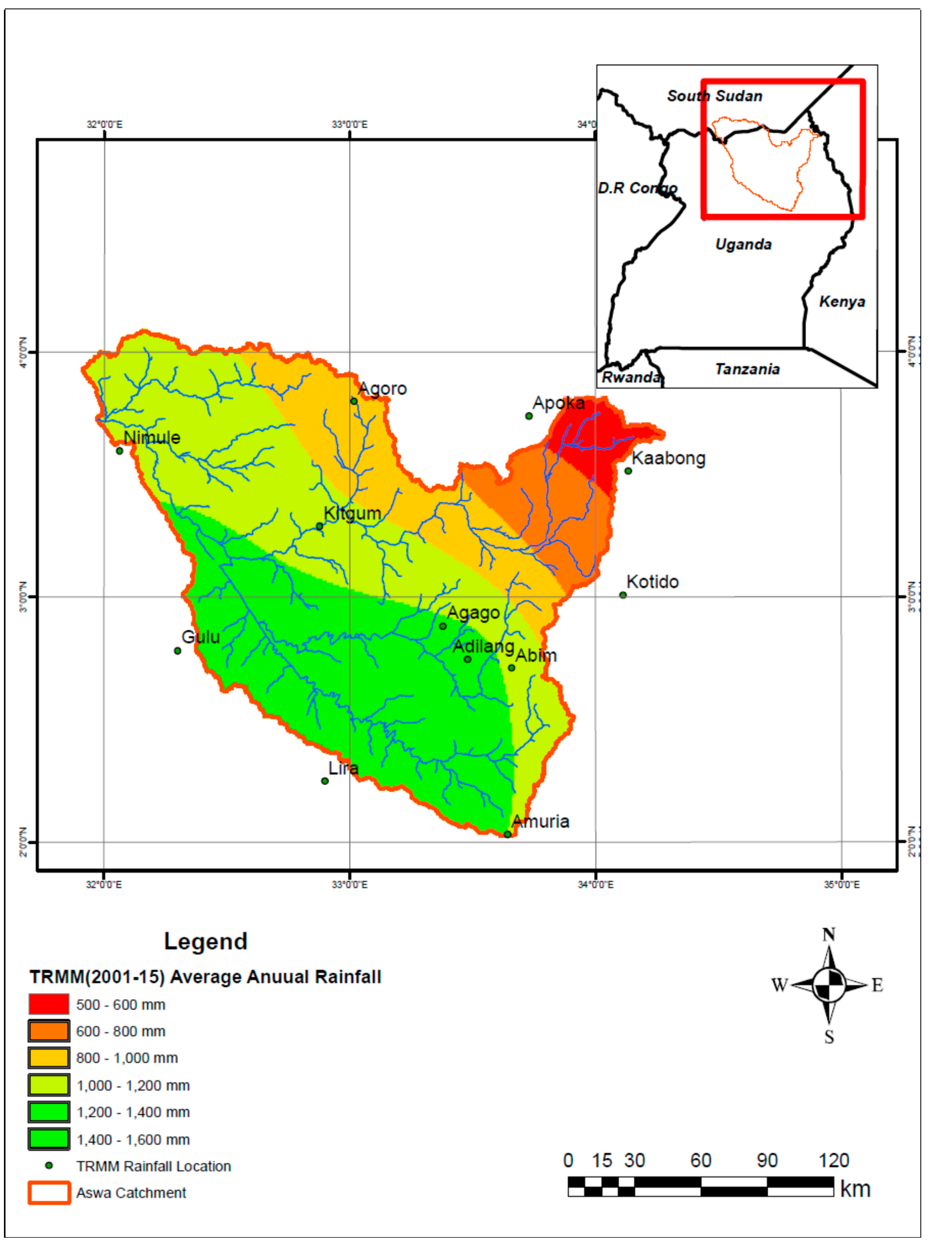
Figure 1.
Location of Aswa River catchment and GIS generated average Tropical Rainfall Measuring Mission (TRMM) annual rainfall (2000–2015) distribution.
Figure 1.
Location of Aswa River catchment and GIS generated average Tropical Rainfall Measuring Mission (TRMM) annual rainfall (2000–2015) distribution.
Figure 2.
Correlation of TRMM and observed rainfall data for Lira.
Figure 2.
Correlation of TRMM and observed rainfall data for Lira.
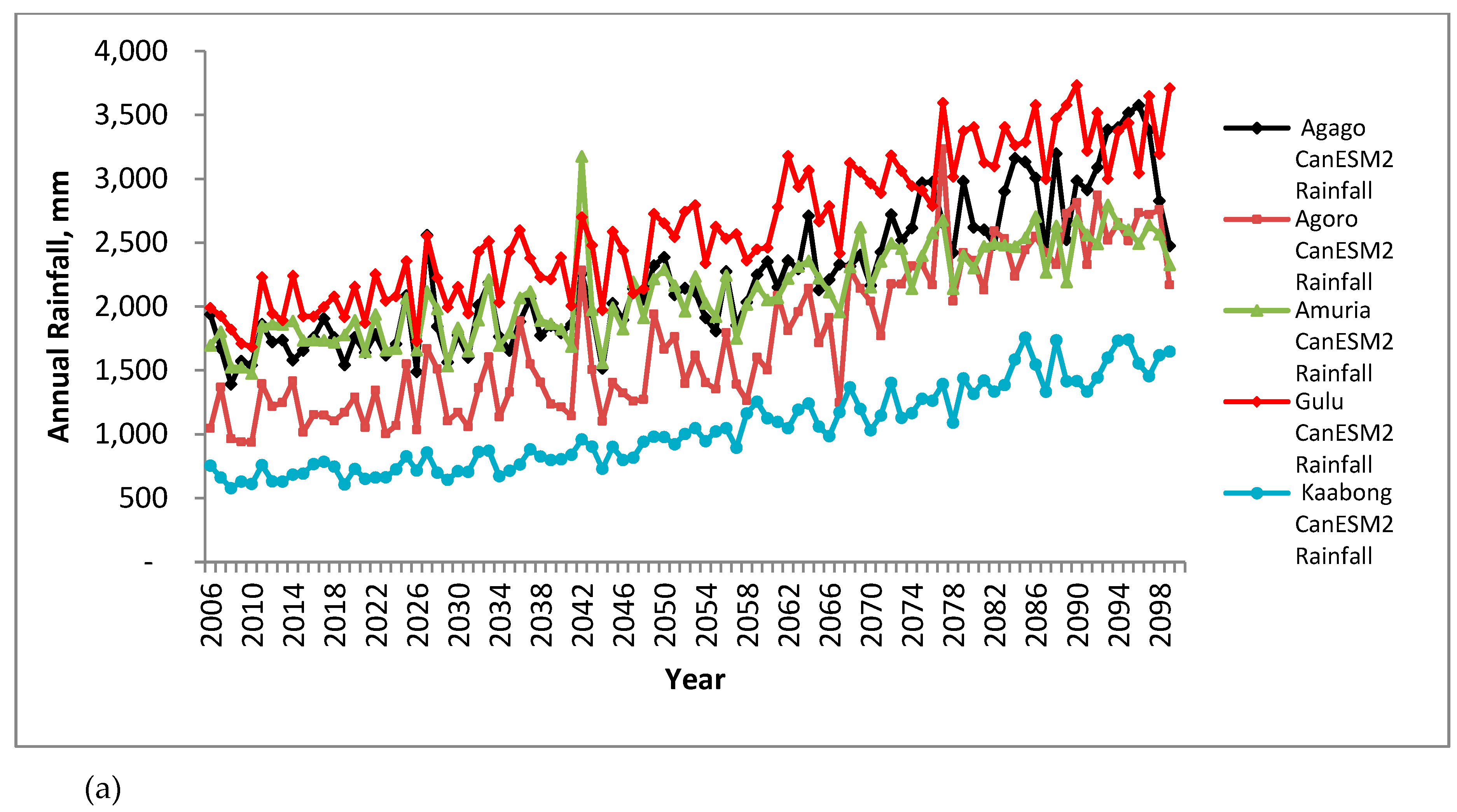
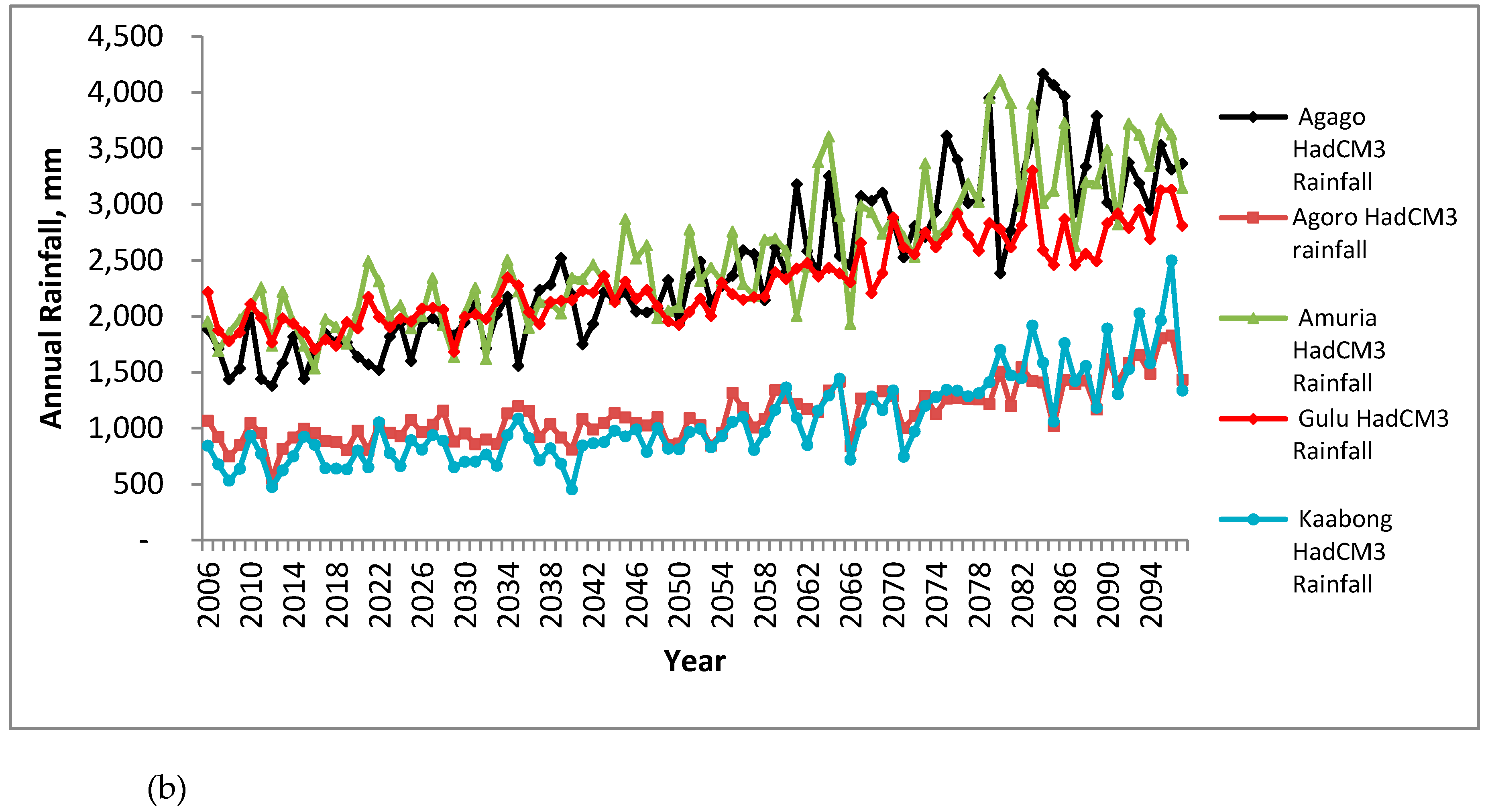
Figure 3.
Simulated future rainfall for Agago, Amuria, Gulu, Agoro and Kaabong locations (a) CanESM2-SDSM (2006–2100) (b) HadCM3-SDSM (2006–2097).
Figure 3.
Simulated future rainfall for Agago, Amuria, Gulu, Agoro and Kaabong locations (a) CanESM2-SDSM (2006–2100) (b) HadCM3-SDSM (2006–2097).
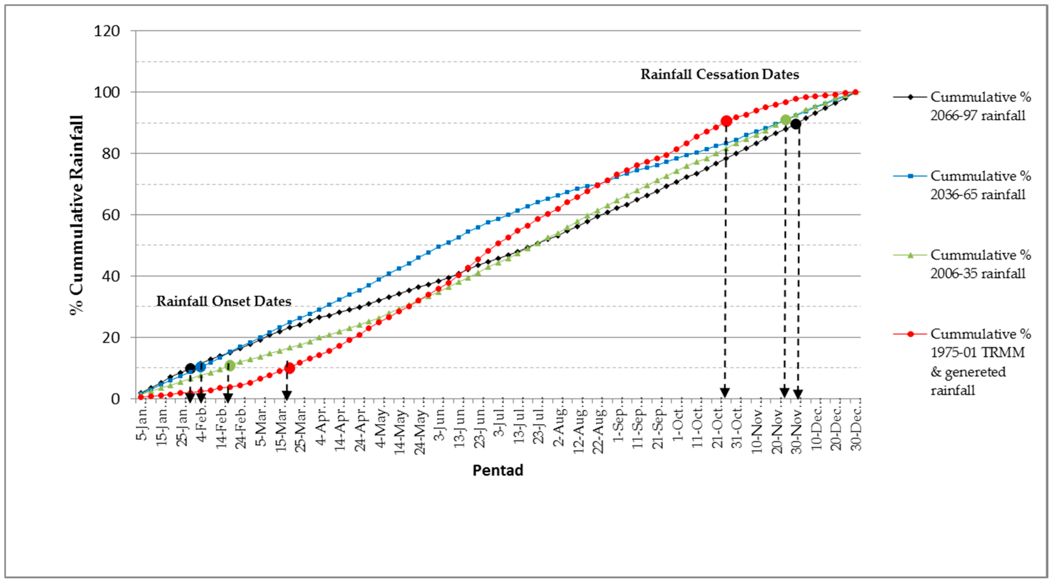
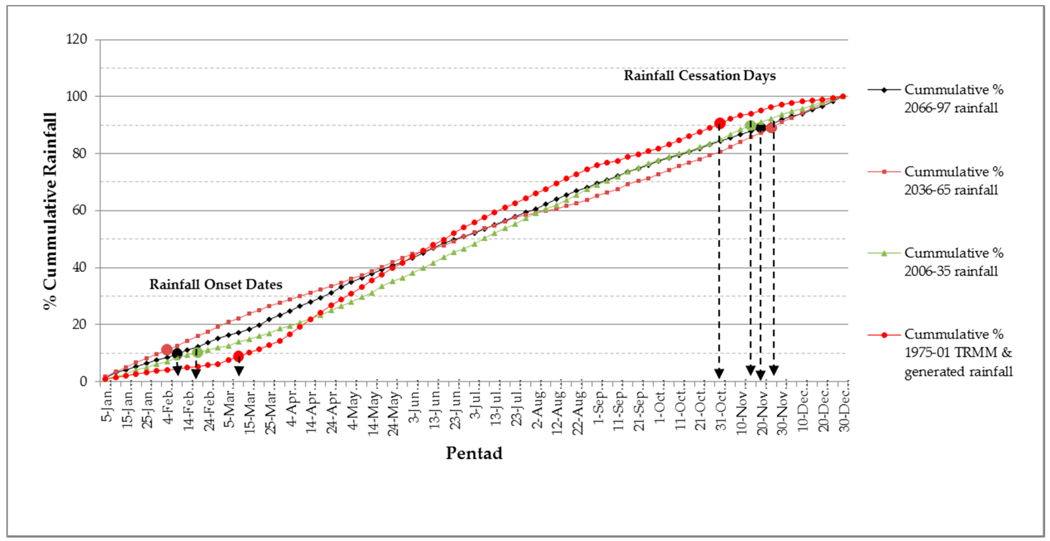
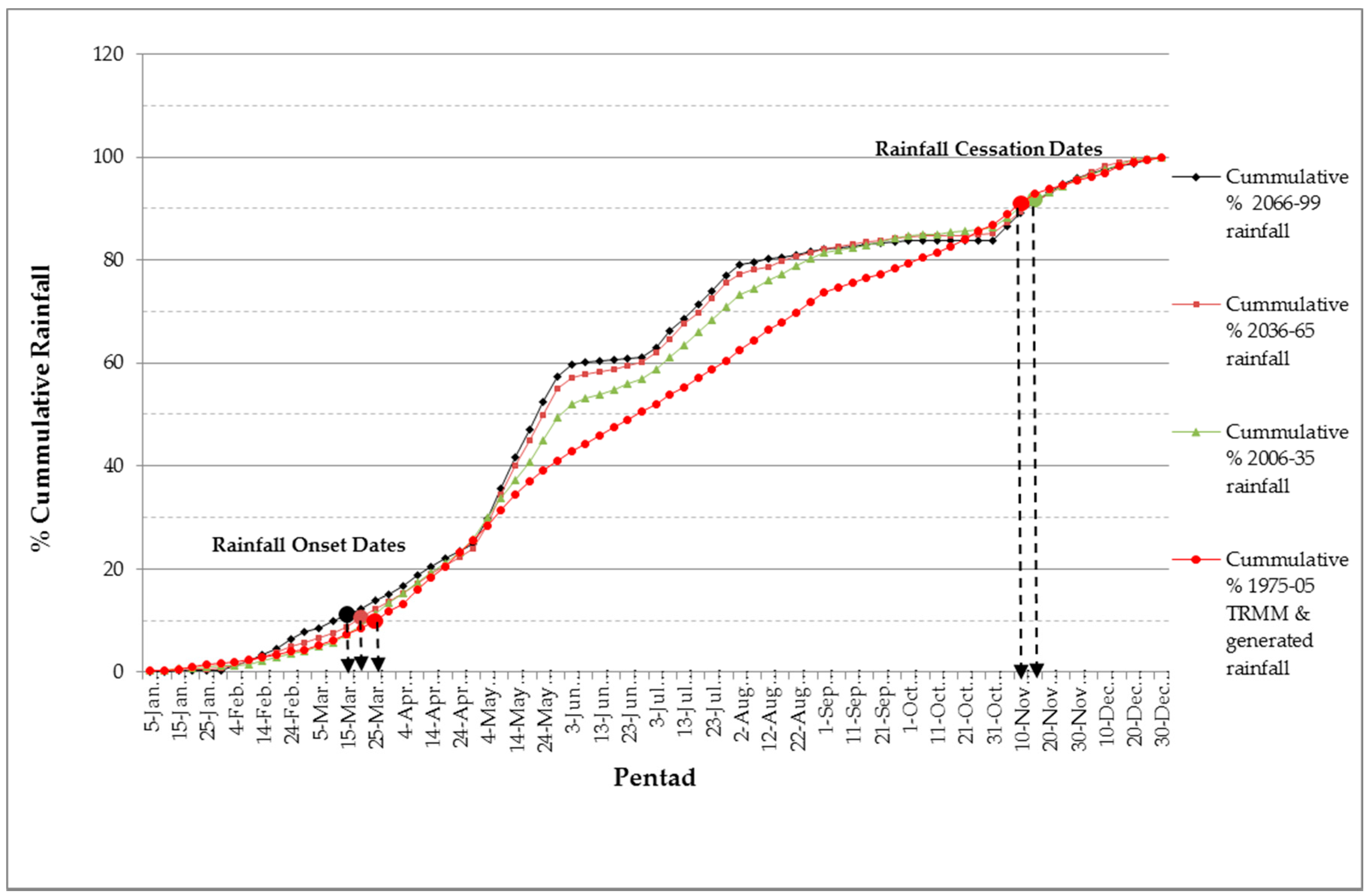
Figure 4.
Agago Future Mean Rainfall Onset and Cessation (TRMM, weather generated Rainfall (1975–2001) and projected (HadCM3) 2006–2035, 2006–2065 and 2006–2099).
Figure 4.
Agago Future Mean Rainfall Onset and Cessation (TRMM, weather generated Rainfall (1975–2001) and projected (HadCM3) 2006–2035, 2006–2065 and 2006–2099).
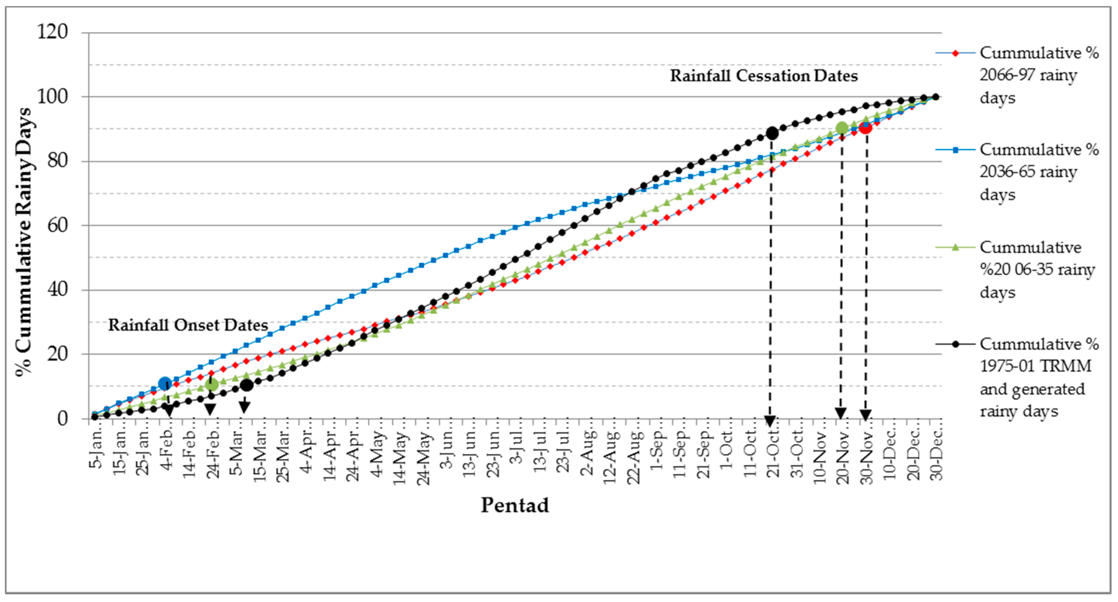
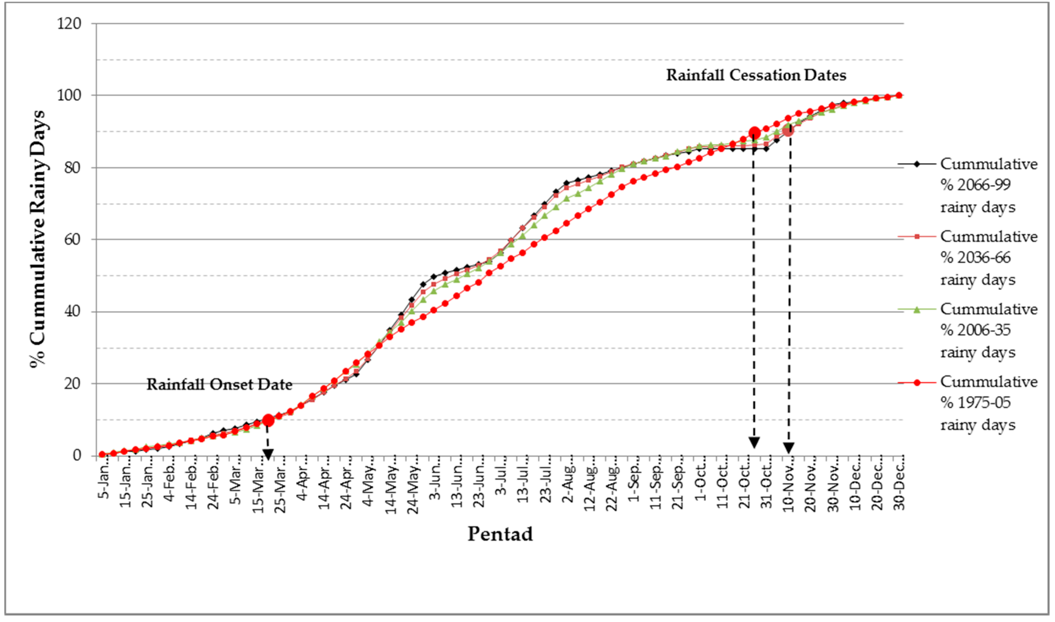
Figure 5.
Agago Future Mean Rainfall Onset and Cessation for Rainy Days (TRMM Rainfall (1975-2001) and projected (HadCM3) 2006–2035, 2006–2065 and 2006–2099).
Figure 5.
Agago Future Mean Rainfall Onset and Cessation for Rainy Days (TRMM Rainfall (1975-2001) and projected (HadCM3) 2006–2035, 2006–2065 and 2006–2099).
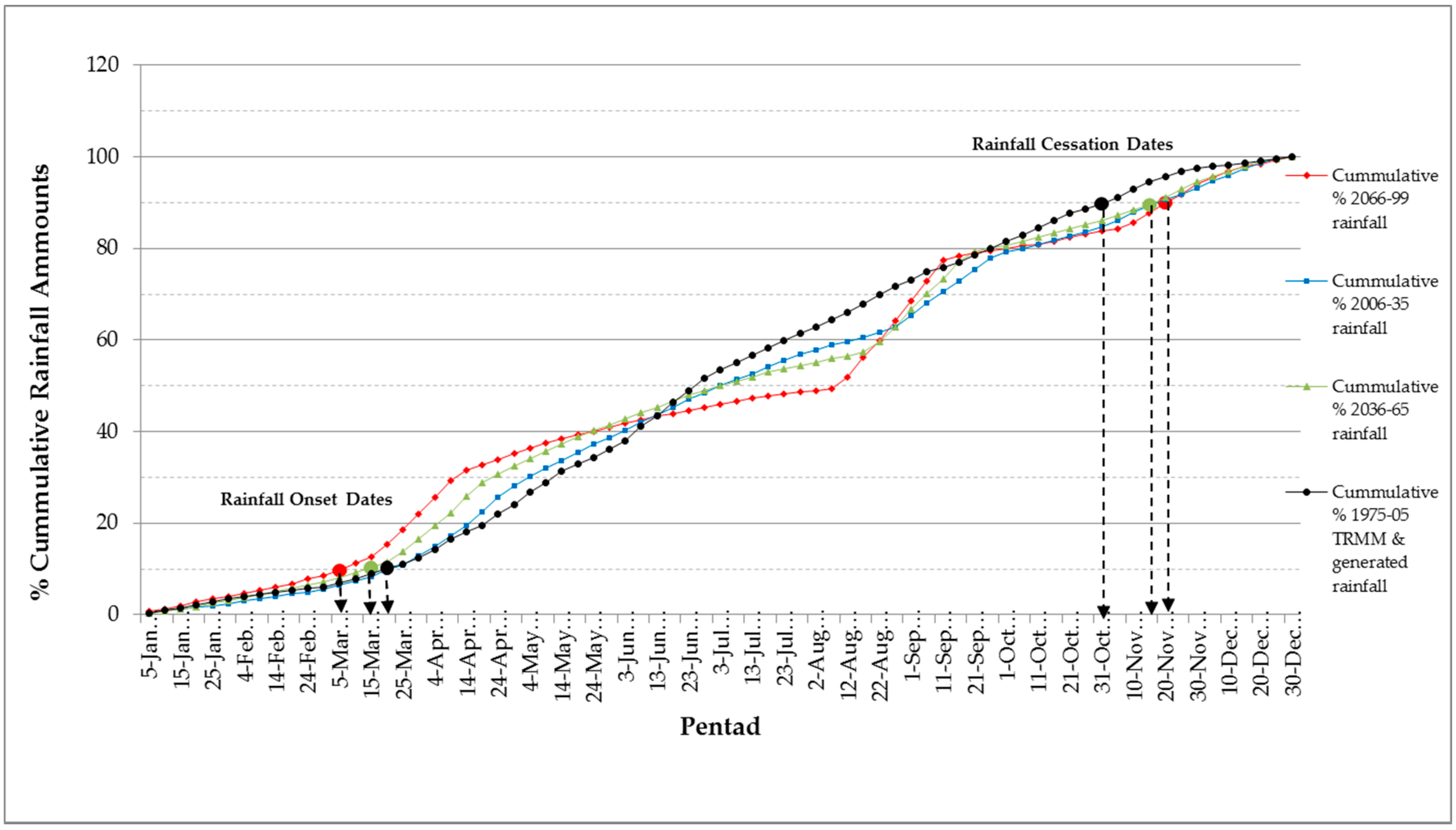
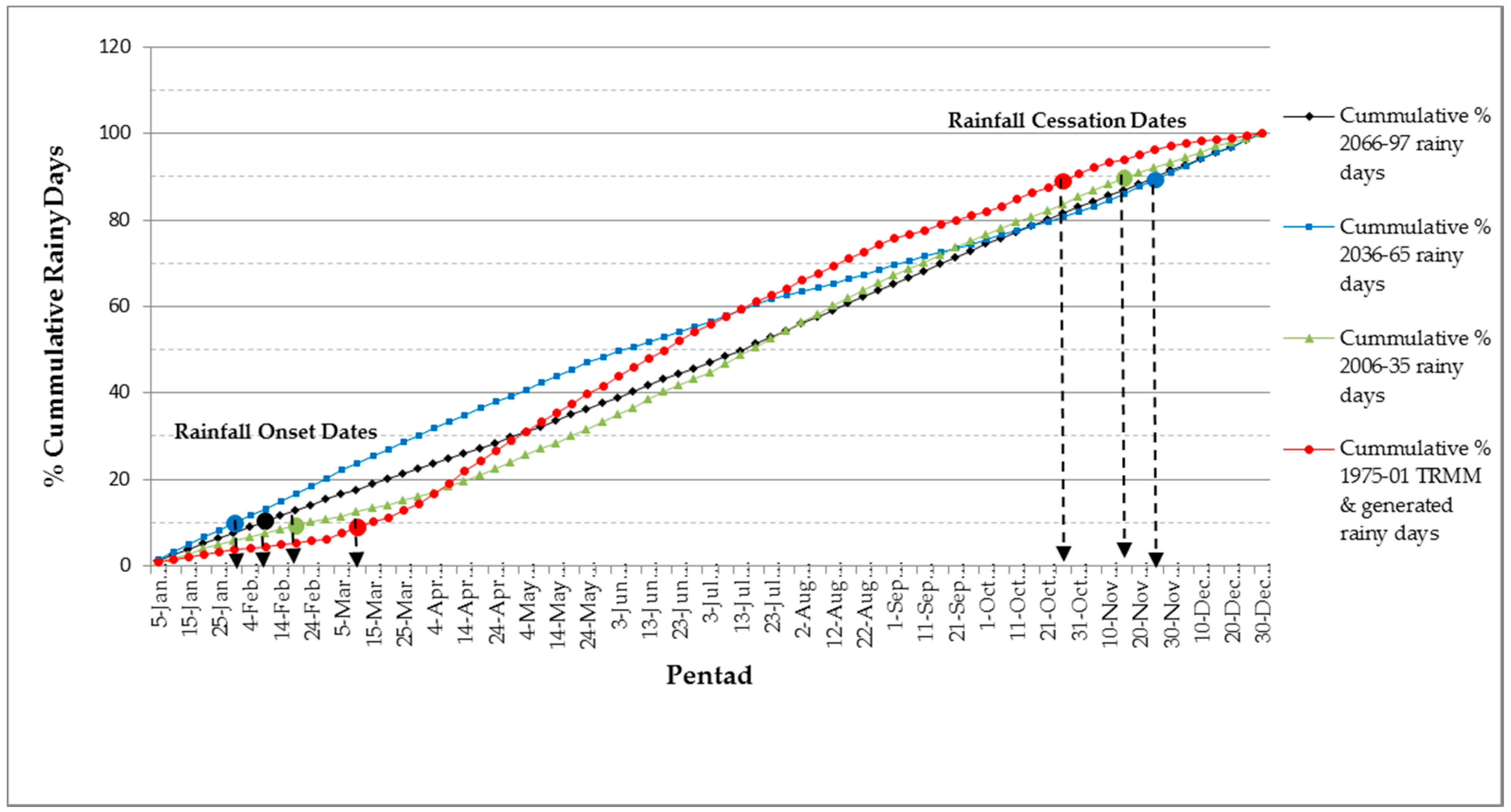
Figure 6.
Agago Future Mean Rainfall Onset and Cessation (TRMM Rainfall (1975–2005) and projected (CanESM2) 2006–2035, 2036–2065 and 2066–2099).
Figure 6.
Agago Future Mean Rainfall Onset and Cessation (TRMM Rainfall (1975–2005) and projected (CanESM2) 2006–2035, 2036–2065 and 2066–2099).
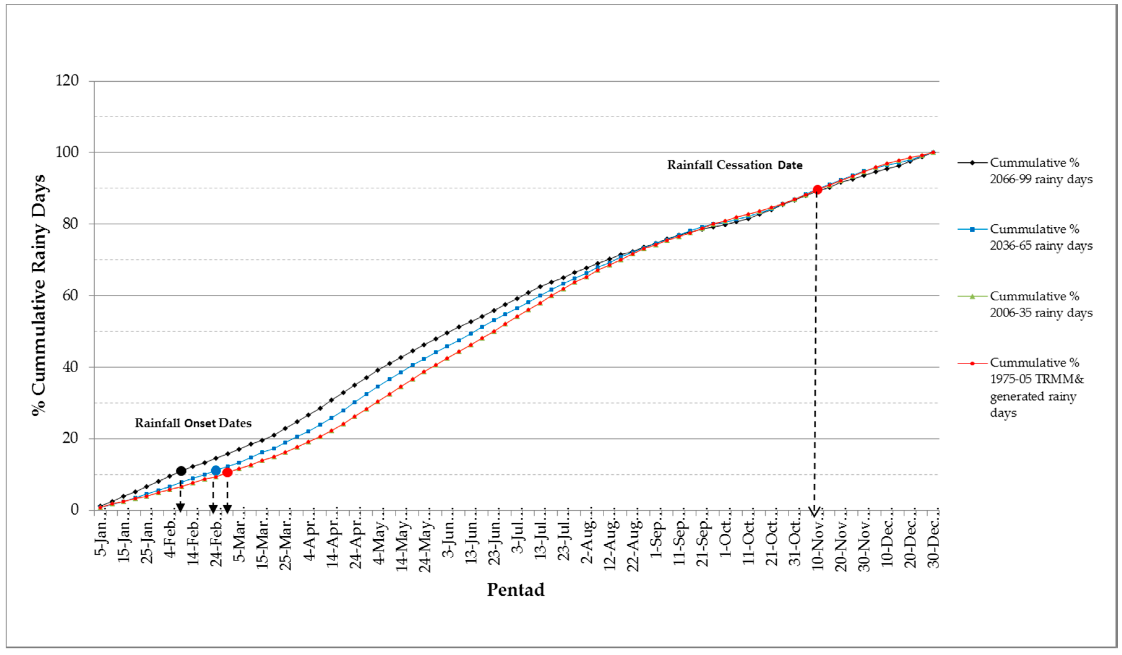
Figure 7.
Agago Future Mean Rainfall Onset and Cessation for Rainy Days (TRMM Rainfall (1975–2005) and projected (CanESM2) 2006–2035, 2036–2065 and 2066–2099).
Figure 7.
Agago Future Mean Rainfall Onset and Cessation for Rainy Days (TRMM Rainfall (1975–2005) and projected (CanESM2) 2006–2035, 2036–2065 and 2066–2099).
Figure 8.
Kaabong Future Mean Rainfall Onset and Cessation Dates (TRMM rainfall (1975–2001) and projected (HadCM3) 2006–2035, 2036–2065 and 2066–2099).
Figure 8.
Kaabong Future Mean Rainfall Onset and Cessation Dates (TRMM rainfall (1975–2001) and projected (HadCM3) 2006–2035, 2036–2065 and 2066–2099).
Figure 9.
Kaabong Future Mean Rainfall Onset and Cessation for Rainy Days (TRMM rainfall (1975–2001) and projected (HadCM3) 2006–2035, 2036–2065 and 2066–2099).
Figure 9.
Kaabong Future Mean Rainfall Onset and Cessation for Rainy Days (TRMM rainfall (1975–2001) and projected (HadCM3) 2006–2035, 2036–2065 and 2066–2099).
Figure 10.
Kaabong Future Mean Rainfall Onset and Cessation Dates (TRMM rainfall (1975–2005) and projected (CanESM2) 2006–2035, 2036–2065 and 2066–2099.
Figure 10.
Kaabong Future Mean Rainfall Onset and Cessation Dates (TRMM rainfall (1975–2005) and projected (CanESM2) 2006–2035, 2036–2065 and 2066–2099.
Figure 11.
Kaabong Future Mean Rainfall Onset and Cessation for Rainy Days (TRMM rainfall (1975–2005) and projected (CanESM2) 2006–2035, 2036–2065 and 2066–2099.
Figure 11.
Kaabong Future Mean Rainfall Onset and Cessation for Rainy Days (TRMM rainfall (1975–2005) and projected (CanESM2) 2006–2035, 2036–2065 and 2066–2099.
Figure 12.
Agoro CanESM2 future average monthly rainfall variations for (a) maximum monthly rainfall and (b) minimum monthly rainfall.
Figure 12.
Agoro CanESM2 future average monthly rainfall variations for (a) maximum monthly rainfall and (b) minimum monthly rainfall.
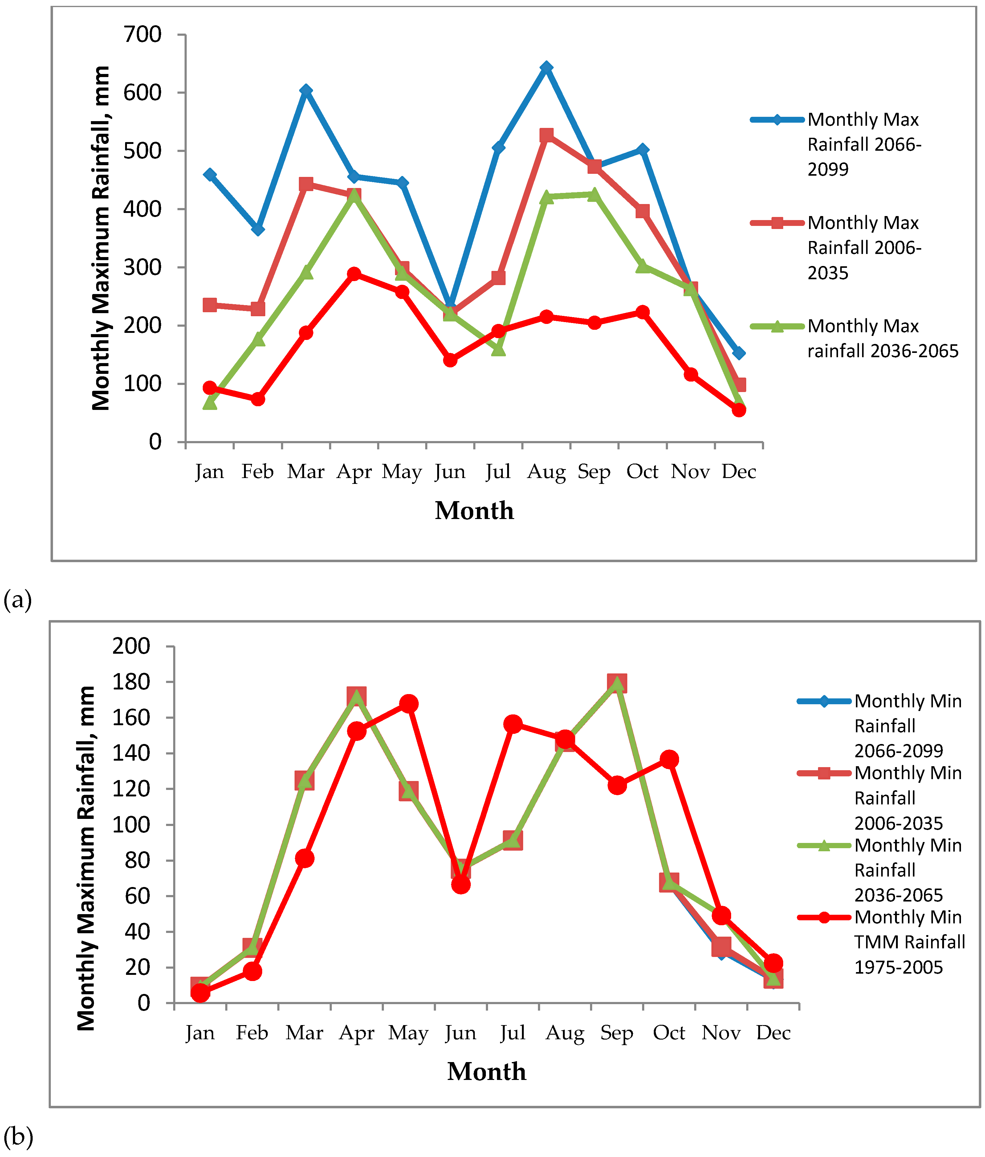
Figure 13.
Gulu CanESM2 future average monthly rainfall variations for (a) maximum monthly rainfall and (b) minimum monthly rainfall.
Figure 13.
Gulu CanESM2 future average monthly rainfall variations for (a) maximum monthly rainfall and (b) minimum monthly rainfall.
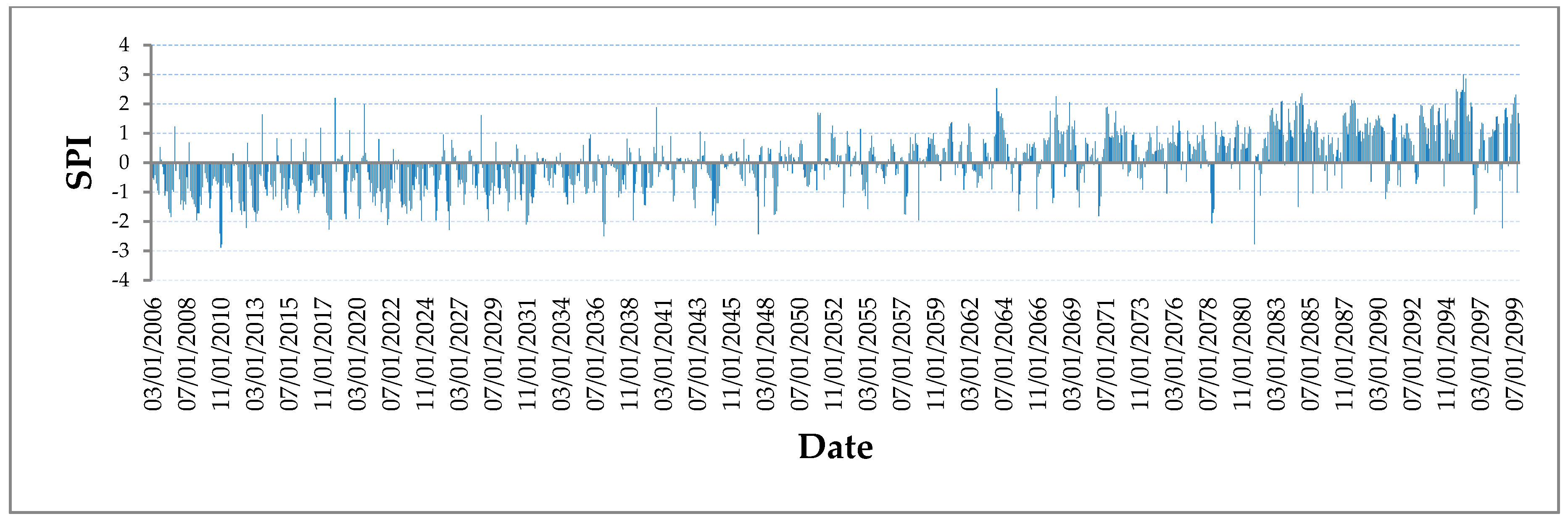
Figure 14.
CanESM2 3-month period SPI values for Kaabong for the duration 2006–2099.
Figure 14.
CanESM2 3-month period SPI values for Kaabong for the duration 2006–2099.
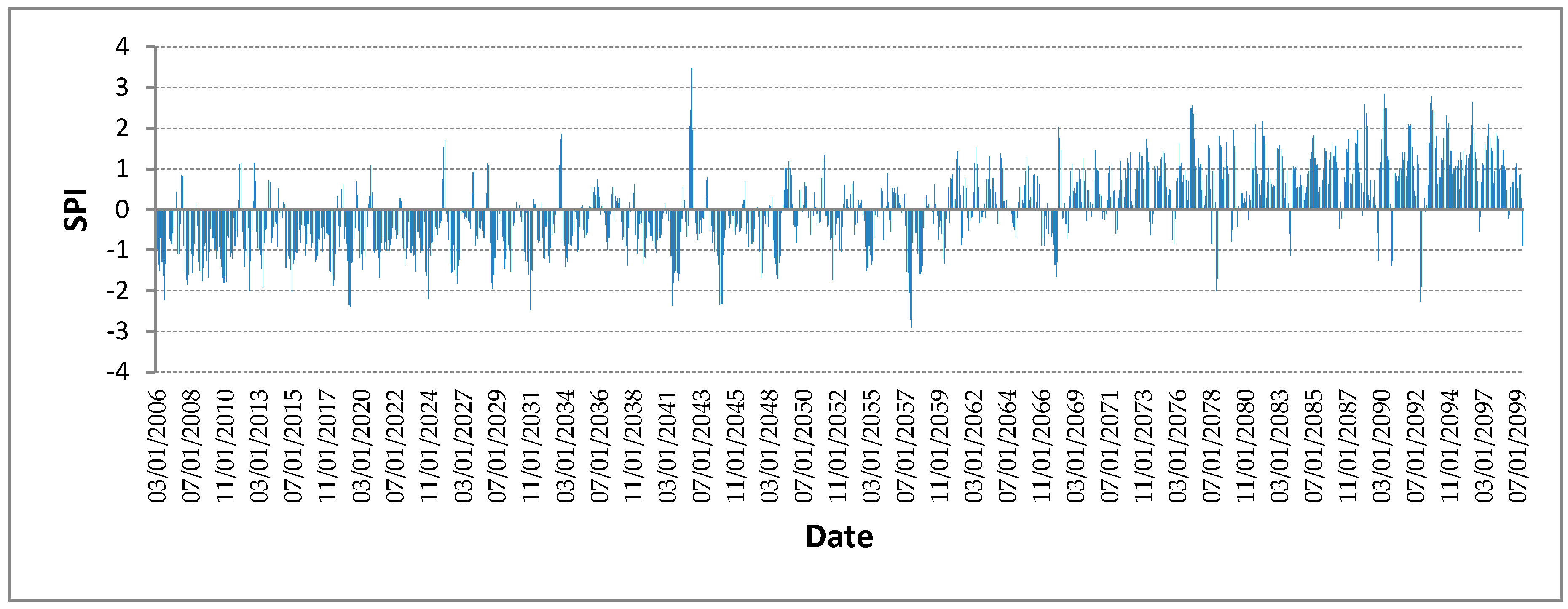
Figure 15.
CanESM2 3-month period SPI values for Agoro for the duration 2006–2099.
Figure 15.
CanESM2 3-month period SPI values for Agoro for the duration 2006–2099.
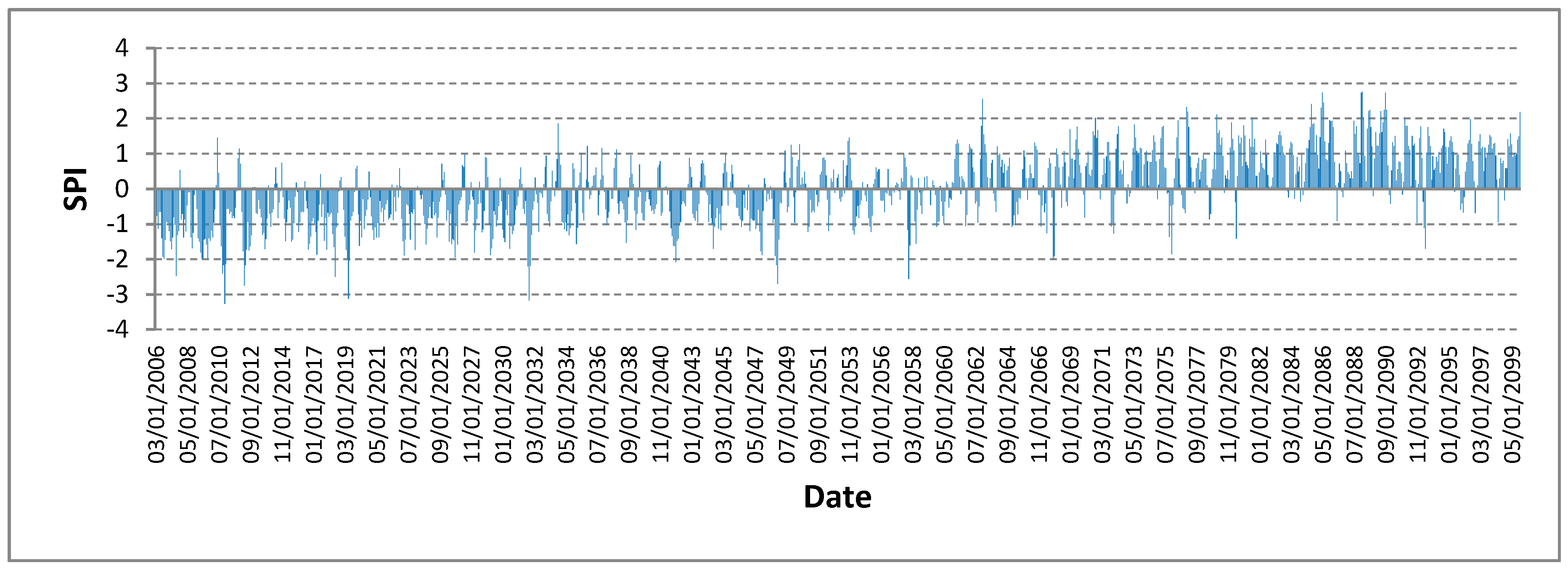
Figure 16.
CanESM2 3-month period SPI values for Gulu for the duration 2006–2099.
Figure 16.
CanESM2 3-month period SPI values for Gulu for the duration 2006–2099.
Table 1.
TRMM rainfall data location points.
Table 1.
TRMM rainfall data location points.
| Location | Latitude, °N | Longitude, °E |
|---|
| Agoro | 3.88 | 33.13 |
| Agago | 2.88 | 33.38 |
| Amuria | 2.13 | 33.63 |
| Kaabong | 3.63 | 33.88 |
| Kitgum | 3.38 | 32.88 |
| Gulu | 2.63 | 32.63 |
| Lira | 2.13 | 33.38 |
| Nimule | 3.63 | 32.13 |
Table 2.
Predictor selection for Kitgum Rainfall.
Table 2.
Predictor selection for Kitgum Rainfall.
| Predictor Description | R1 | P.r | P | PRP = ((P.r − R1)/R1) | P.r | P | PRP = ((P.r − R1)/R1) | P.r | P | PRP = ((P.r − R1)/R1) | P.r | P | PRP = ((P.r − R1)/R1) | Rank |
|---|
| Mean temperature at 2 m | 0.59 | | | | | | | | | | | | | Super Predictor |
| Surface specific humidity | 0.54 | 0.29 | 0.00 | 0.46 | 0.19 | 0.00 | 0.64 | 0.07 | 0.00 | 0.87 | 0.03 | 0.07 | 0.94 | |
| 850 hPa zonal velocity | 0.52 | 0.37 | 0.00 | 0.29 | | | | | | | | | | 2nd |
| Specific humidity at 850 hPa | 0.50 | 0.31 | 0.00 | 0.39 | 0.22 | 0.00 | 0.55 | | | | | | | 3rd |
| Surface zonal velocity | 0.49 | 0.32 | 0.00 | 0.36 | 0.10 | 0.00 | 0.79 | 0.12 | 0.00 | 0.76 | 0.10 | 0.00 | 0.79 | |
| 850 hPa airflow strength | 0.45 | 0.31 | 0.00 | 0.30 | 0.07 | 0.00 | 0.84 | 0.09 | 0.00 | 0.79 | 0.08 | 0.00 | 0.83 | |
| Surface airflow strength | 0.44 | 0.26 | 0.00 | 0.40 | 0.09 | 0.00 | 0.80 | 0.11 | 0.00 | 0.76 | 0.09 | 0.00 | 0.79 | |
| Specific humidity at 500 hPa | 0.43 | 0.24 | 0.00 | 0.44 | 0.19 | 0.00 | 0.55 | 0.10 | 0.00 | 0.76 | 0.12 | 0.00 | 0.74 | 5th |
| precipitation | 0.37 | 0.17 | 0.00 | 0.53 | 0.04 | 0.01 | 0.89 | 0.10 | 0.00 | 0.72 | | | | 4th |
Table 3.
Calibration and validation of Statistical down Scaling Model (SDSM) results for various locations within the Aswa catchment.
Table 3.
Calibration and validation of Statistical down Scaling Model (SDSM) results for various locations within the Aswa catchment.
| Location | GCM | Parameter | Process | Bias | Regression Statistics | ANOVA |
|---|
| | | Rainfall | | Period | | R | R2 | Standard Error | Observations | F | Significance of F |
| Agago | HadCM3 | | Calibration | 1975–1990(16yrs) | 1.034 | 0.87 | 0.76 | 29.25 | 192 | 612 | 2.58 × 10−61 |
| | | | Validation | 1991–2001(11yrs) | 0.988 | 0.88 | 0.77 | 26.93 | 132 | 430 | 4.61 × 10−43 |
| | CanESM2 | | Calibration | 1975–1990(16yrs) | 1.021 | 0.97 | 0.95 | 13.84 | 192 | 3535 | 1.00 × 10−124 |
| | | | Validation | 1991–2005(15yrs) | 1.010 | 0.97 | 0.95 | 12.64 | 180 | 3167 | 2.54 × 10−115 |
| Agoro | HadCM3 | | Calibration | 1975–1990(16yrs) | 1.048 | 0.85 | 0.72 | 21.03 | 192 | 494 | 1.01 × 10−54 |
| | | | Validation | 1991–2001(11yrs) | 0.996 | 0.93 | 0.86 | 14.11 | 132 | 783 | 7.11 × 10−57 |
| | CanESM2 | | Calibration | 1975–1990(16yrs) | 0.964 | 0.95 | 0.90 | 12.33 | 192 | 1797 | 8.59 × 10−99 |
| | | | Validation | 1991–2005(15yrs) | 1.011 | 0.91 | 0.83 | 15.43 | 180 | 842 | 2.10 × 10−69 |
| Amuria | HadCM3 | | Calibration | 1975–1990(16yrs) | 1.030 | 0.87 | 0.76 | 26.82 | 192 | 608 | 3.94 × 10−61 |
| | | | Validation | 1991–2001(11yrs) | 1.055 | 0.86 | 0.74 | 26.43 | 132 | 377 | 2.92 × 10−40 |
| | CanESM2 | | Calibration | 1975–1990(16yrs) | 1.044 | 0.94 | 0.88 | 19.36 | 192 | 1342 | 4.79 × 10−88 |
| | | | Validation | 1991–2005(15yrs) | 1.057 | 0.95 | 0.90 | 16.15 | 180 | 1644 | 7.80 × 10−92 |
| Kaabong | HadCM3 | | Calibration | 1975–1990(16yrs) | 0.995 | 0.90 | 0.81 | 15.44 | 192 | 812 | 1.67 × 10−70 |
| | | | Validation | 1991–2001(11yrs) | 1.136 | 0.83 | 0.69 | 15.75 | 132 | 288 | 9.52 × 10⁻³⁵ |
| | CanESM2 | | Calibration | 1975–1990(16yrs) | 0.980 | 0.95 | 0.89 | 11.59 | 192 | 1587 | 3.49 × 10−94 |
| | | | Validation | 1991–2005(15yrs) | 0.966 | 0.94 | 0.89 | 9.62 | 180 | 1372 | 1.38 × 10−85 |
| Gulu | HadCM3 | | Calibration | 1975–1990(16yrs) | 1.019 | 0.96 | 0.92 | 19.19 | 192 | 2248 | 3.12 × 10−107 |
| | | | Validation | 1991–2001(11yrs) | 0.982 | 0.93 | 0.87 | 23.21 | 132 | 885 | 7.40 × 10−60 |
| | CanESM2 | | Calibration | 1975–1990(16yrs) | 1.019 | 0.97 | 0.95 | 15.45 | 192 | 3574 | 3.73 × 10−125 |
| | | | Validation | 1991–2005(16yrs) | 0.998 | 0.96 | 0.92 | 18.18 | 180 | 2009 | 6.77 × 10−99 |
Table 4.
Classification of SPI values.
Table 4.
Classification of SPI values.
| SPI Value | Class |
|---|
| 2.00 or more | Extremely wet |
| 1.50–1.99 | Severely wet |
| 1.00–1.49 | Moderately wet |
| 0–0.99 | Mildly wet |
| 0 to −0.99 | Mildly dry |
| −1.00 to −1.49 | Moderately dry |
| −1.50 to −1.99 | Severely dry |
| −2 or less | Extremely dry |
Table 5.
Results of Homogeneity Test and Mann–Kendall Statistics for TRMM and Simulated Rainfall Data for Agoro and Amuria Locations in Aswa Catchment. SNHT = standard normal homogeneity test.
Table 5.
Results of Homogeneity Test and Mann–Kendall Statistics for TRMM and Simulated Rainfall Data for Agoro and Amuria Locations in Aswa Catchment. SNHT = standard normal homogeneity test.
| | Homogeneity Test-SNHT | Mann–Kendall Statistics |
|---|
GCM,
Location | Data Type | Period | p-Value (Two-Tailed) | Alpha | Comment | Number of Observations | Kendall’s Tau | Sen’s Slope | Comment |
|---|
| CanESM2 | | | | | | | | | |
| Agoro | TRMM and generated monthly Rainfall | 1975–2005 | 0.099 | 0.05 | p > α (0.05), homogeneous | 372 | | | |
| | TRMM and simulated annual Rainfall | 2006–2099 | | | | 94 | 0.683 | 18.52 | Positive trend |
| | TRMM and simulated annual Rainfall | 2006–2065 | | | | 60 | 0.449 | 10.42 | Positive trend |
| | TRMM and simulated annual Rainfall | 2006–2035 | | | | 30 | 0.200 | 6.628 | Positive trend |
| HadCM3 | | | | | | | | | |
| Agoro | TRMM and simulated annual Rainfall | 2006–2097 | | | | 92 | 0.669 | 3.219 | Positive trend |
| | TRMM and simulated annual Rainfall | 2006–2065 | | | | 60 | 0.463 | 2.339 | Positive trend |
| | TRMM and simulated annual Rainfall | 2006–2035 | | | | 30 | 0.195 | 1.426 | Positive trend |
| CanESM2 | | | | | | | | | |
| Amuria | TRMM and generated monthly Rainfall | 1975–2005 | 0.220 | 0.05 | p > α (0.05), homogeneous | 372 | | | |
| | TRMM and simulated annual Rainfall | 2006–2100 | | | | 94 | 0.647 | 10.52 | Positive trend |
| | TRMM and simulated annual Rainfall | 2006–2065 | | | | 60 | 0.472 | 9.072 | Positive trend |
| | TRMM and simulated annual Rainfall | 2006–2035 | | | | 30 | 0.172 | 6.286 | Positive trend |
| HadCM3 | | | | | | | | | |
| Amuria | TRMM and simulated annual Rainfall | 2001–2097 | | | | 92 | 0.647 | 18.54 | Positive trend |
| | TRMM and simulated annual Rainfall | 2001–2065 | | | | 60 | 0.482 | 13.70 | Positive trend |
| | TRMM and simulated annual Rainfall | 2001–2035 | | | | 30 | 0.218 | 9.212 | Positive trend |
Table 6.
Agoro TRMM and Simulated (CanESM2and Had3) Monthly Rainfall Coefficient of Variation.
Table 6.
Agoro TRMM and Simulated (CanESM2and Had3) Monthly Rainfall Coefficient of Variation.
| | Jan. | Feb. | Mar. | Apr. | May | Jun. | Jul. | Aug. | Sep. | Oct. | Nov. | Dec. |
|---|
| CanESM2 | | | | | | | | | | | | |
| 1975–2005 TRMM and Weather Generator |
| Mean | 24.2 | 28.4 | 48.2 | 116.9 | 74.1 | 83.2 | 108.9 | 117.3 | 55.9 | 83.8 | 65.9 | 25.0 |
| Standard Deviation | 18.4 | 23.0 | 10.6 | 24.1 | 18.8 | 13.7 | 11.1 | 23.6 | 13.4 | 15.5 | 28.1 | 10.0 |
| CV, % | 76.1 | 80.8 | 22.0 | 20.6 | 25.3 | 16.5 | 10.2 | 20.1 | 24.0 | 18.5 | 42.7 | 40.1 |
| 2006–2035 TRMM and Simulation |
| Mean | 21.5 | 58.0 | 84.0 | 164.2 | 123.6 | 79.9 | 56.2 | 191.4 | 159.4 | 56.6 | 166.3 | 52.9 |
| Standard Deviation | 7.2 | 55.8 | 38.6 | 52.9 | 37.4 | 23.8 | 16.4 | 30.0 | 51.8 | 27.8 | 92.7 | 20.6 |
| CV | 33.4 | 96.3 | 46.0 | 32.2 | 30.3 | 29.7 | 29.1 | 15.7 | 32.5 | 49.0 | 55.7 | 38.9 |
| 2006–2065 TRMM and Simulation |
| Mean | 24.2 | 96.6 | 107.2 | 209.9 | 145.8 | 97.2 | 47.7 | 195.1 | 197.9 | 58.1 | 160.8 | 49.8 |
| Standard Deviation | 8.3 | 110.3 | 72.5 | 80.6 | 40.2 | 36.1 | 15.7 | 33.3 | 74.0 | 68.8 | 91.2 | 18.5 |
| CV | 34.4 | 114.1 | 67.7 | 38.4 | 27.6 | 37.1 | 32.8 | 17.1 | 37.4 | 118.5 | 56.7 | 37.1 |
| 2006–2099 TRMM and Simulation |
| Mean | 28.7 | 224.0 | 150.0 | 246.5 | 176.3 | 128.8 | 40.4 | 206.1 | 271.7 | 54.4 | 171.0 | 47.9 |
| Standard Deviation | 14.2 | 255.4 | 94.9 | 103.5 | 59.9 | 60.9 | 16.6 | 34.5 | 126.7 | 62.1 | 101.5 | 16.6 |
| CV, % | 49.4 | 114.0 | 63.3 | 42.0 | 34.0 | 47.3 | 41.1 | 16.7 | 46.6 | 114.0 | 59.4 | 34.7 |
| HadCM3 | | | | | | | | | | | | |
| 1975–2001 TRMM and Weather Generator |
| Mean | 46.6 | 38.6 | 49.1 | 62.7 | 74.1 | 73.6 | 101.8 | 101.0 | 92.9 | 86.3 | 74.7 | 55.8 |
| Standard Deviation | 26.5 | 21.5 | 32.0 | 44.8 | 42.4 | 30.3 | 34.7 | 26.6 | 28.2 | 23.8 | 35.3 | 33.0 |
| CV, % | 56.9 | 55.7 | 65.1 | 71.3 | 57.2 | 41.1 | 34.0 | 26.3 | 30.3 | 27.6 | 47.2 | 59.1 |
| 2006–2035 TRMM and Simulation |
| Mean | 46.6 | 38.6 | 49.1 | 62.7 | 74.1 | 73.6 | 101.8 | 101.0 | 92.9 | 86.3 | 74.7 | 55.8 |
| Standard Deviation | 26.5 | 21.5 | 32.0 | 44.8 | 42.4 | 30.3 | 34.7 | 26.6 | 28.2 | 23.8 | 35.3 | 33.0 |
| CV, % | 56.9 | 55.7 | 65.1 | 71.3 | 57.2 | 41.1 | 34.0 | 26.3 | 30.3 | 27.6 | 47.2 | 59.1 |
| 2006–2065 TRMM ans Simulation |
| Mean | 66.9 | 73.7 | 83.7 | 83.8 | 89.2 | 76.9 | 78.9 | 69.6 | 61.9 | 67.3 | 72.0 | 67.7 |
| Standard Deviation | 39.7 | 53.3 | 54.4 | 49.0 | 45.6 | 41.8 | 44.3 | 42.9 | 40.9 | 42.4 | 45.3 | 40.0 |
| CV, % | 59.4 | 72.3 | 65.0 | 58.5 | 51.1 | 54.4 | 56.1 | 61.6 | 66.0 | 63.0 | 62.9 | 59.2 |
| 2006–2097 TRMM and Simulation |
| Mean | 77.7 | 67.2 | 67.4 | 65.6 | 76.3 | 74.6 | 80.5 | 85.4 | 89.5 | 89.8 | 90.4 | 83.6 |
| Standard Deviation | 57.9 | 52.7 | 53.6 | 50.7 | 52.0 | 47.2 | 46.0 | 57.1 | 66.3 | 61.5 | 64.7 | 55.3 |
| CV, % | 74.5 | 78.4 | 79.5 | 77.3 | 68.1 | 63.3 | 57.1 | 66.9 | 74.1 | 68.5 | 71.6 | 66.1 |
Table 7.
Kaabong TRMM and Simulated (CanESM2and HadCM3) Monthly Rainfall Coefficient of Variation.
Table 7.
Kaabong TRMM and Simulated (CanESM2and HadCM3) Monthly Rainfall Coefficient of Variation.
| | Jan. | Feb. | Mar. | Apr. | May | Jun. | Jul. | Aug. | Sep. | Oct. | Nov. | Dec. |
|---|
| CanESM2 | | | | | | | | | | | | |
| 1975–2005 TRMM and Weather Generator |
| Mean | 9.9 | 12.4 | 47.5 | 76.2 | 90.4 | 51.5 | 63.9 | 67.0 | 28.8 | 40.5 | 43.9 | 24.4 |
| Standard Deviation | 6.4 | 4.6 | 16.1 | 15.5 | 35.5 | 14.0 | 7.5 | 19.6 | 9.5 | 13.7 | 17.6 | 16.4 |
| CV, % | 65.1 | 36.8 | 33.8 | 20.3 | 39.3 | 27.1 | 11.8 | 29.3 | 33.0 | 33.7 | 40.1 | 67.5 |
| 2006–2035 TRMM and Simulation |
| Mean | 7.3 | 21.0 | 70.3 | 92.8 | 172.8 | 41.7 | 111.1 | 61.6 | 24.8 | 12.2 | 58.1 | 34.2 |
| Standard Deviation | 1.2 | 9.6 | 23.5 | 18.5 | 41.8 | 11.7 | 23.1 | 19.6 | 5.5 | 6.6 | 15.5 | 15.9 |
| CV, % | 16.2 | 45.7 | 33.4 | 20.0 | 24.2 | 28.2 | 20.8 | 31.8 | 22.2 | 54.1 | 26.7 | 46.5 |
| 2006–2065 TRMM ans Simulation |
| Mean | 7.3 | 37.2 | 77.7 | 101.0 | 239.2 | 39.2 | 133.5 | 55.1 | 24.2 | 8.3 | 76.3 | 38.0 |
| Standard Deviation | 1.2 | 26.1 | 32.3 | 24.0 | 87.8 | 10.9 | 35.0 | 18.8 | 5.1 | 6.7 | 32.1 | 17.7 |
| CV, % | 15.7 | 70.1 | 41.6 | 23.7 | 36.7 | 27.9 | 26.2 | 34.1 | 21.0 | 81.2 | 42.1 | 46.5 |
| 2006–2099 TRMM and Simulation |
| Mean | 7.2 | 64.5 | 91.2 | 114.1 | 322.5 | 34.5 | 172.8 | 51.6 | 23.6 | 5.8 | 107.7 | 43.2 |
| Standard Deviation | 1.8 | 48.3 | 38.5 | 31.8 | 139.1 | 12.1 | 66.3 | 18.2 | 5.1 | 6.5 | 67.5 | 21.2 |
| CV, % | 25.2 | 74.9 | 42.3 | 27.8 | 43.1 | 35.1 | 38.4 | 35.3 | 21.6 | 111.8 | 62.6 | 49.1 |
| HadCM3 | | | | | | | | | | | | |
| 1975–2001 TRMM and Weather Generator |
| Mean | 11.2 | 14.6 | 68.7 | 85.3 | 102.6 | 56.0 | 52.1 | 66.4 | 25.4 | 51.1 | 62.8 | 27.5 |
| Standard Deviation | 3.7 | 4.3 | 20.0 | 9.1 | 30.5 | 10.2 | 5.3 | 5.4 | 3.0 | 6.7 | 12.6 | 12.3 |
| CV, % | 32.9 | 29.2 | 29.2 | 10.6 | 29.7 | 18.3 | 10.3 | 8.1 | 11.8 | 13.2 | 20.0 | 44.8 |
| 2006–2035 TRMM and Simulation |
| Mean | 49.1 | 51.2 | 66.0 | 77.1 | 87.6 | 90.7 | 102.6 | 96.4 | 80.4 | 74.5 | 73.9 | 62.4 |
| Standard Deviation | 25.8 | 39.0 | 48.6 | 62.0 | 60.4 | 40.3 | 34.3 | 41.5 | 32.4 | 30.3 | 23.5 | 32.8 |
| CV, % | 52.5 | 76.2 | 73.7 | 80.4 | 69.0 | 44.4 | 33.5 | 43.1 | 40.4 | 40.6 | 31.8 | 52.6 |
| 2006–2065 TRMM and Simulation |
| Mean | 88.4 | 86.6 | 93.9 | 88.3 | 103.1 | 101.0 | 97.8 | 92.2 | 94.2 | 95.2 | 100.9 | 97.8 |
| Standard Deviation | 58.2 | 58.4 | 53.9 | 52.1 | 63.1 | 38.5 | 35.8 | 46.0 | 75.7 | 71.9 | 69.1 | 72.2 |
| CV, % | 65.9 | 67.5 | 57.4 | 59.0 | 61.3 | 38.1 | 36.6 | 49.9 | 80.3 | 75.6 | 68.5 | 73.8 |
| 2006–2097 TRMM and Simulation |
| Mean | 120.8 | 109.8 | 127.7 | 127.5 | 135.1 | 135.8 | 130.1 | 128.3 | 120.0 | 117.3 | 123.6 | 132.8 |
| Standard Deviation | 79.1 | 78.7 | 100.2 | 109.6 | 96.3 | 115.7 | 83.7 | 81.0 | 80.6 | 75.3 | 87.6 | 89.9 |
| CV, % | 65.5 | 71.7 | 78.5 | 86.0 | 71.3 | 85.2 | 64.3 | 63.1 | 67.2 | 64.2 | 70.8 | 67.7 |
Table 8.
Gulu TRMM and Simulated (CanESM2and HadCM3) Monthly Rainfall Coefficient of Variation.
Table 8.
Gulu TRMM and Simulated (CanESM2and HadCM3) Monthly Rainfall Coefficient of Variation.
| | Jan. | Feb. | Mar. | Apr. | May | Jun. | Jul. | Aug. | Sep. | Oct. | Nov. | Dec. |
|---|
| CanESM2 | | | | | | | | | | | | |
| 2006–2099 TRMM and Simulation |
| Mean | 82.4 | 141.7 | 297.9 | 314.1 | 253.4 | 153.8 | 220.3 | 380.4 | 323.2 | 278.9 | 137.4 | 42.8 |
| Standard Deviation | 86.5 | 84.6 | 116.3 | 63.4 | 63.0 | 34.1 | 117.7 | 109.2 | 61.2 | 88.4 | 51.6 | 26.6 |
| CV, % | 105.0 | 59.7 | 39.0 | 20.2 | 24.9 | 22.2 | 53.4 | 28.7 | 18.9 | 31.7 | 37.6 | 62.3 |
| 2006–2065 TRMM and Simulation |
| Mean | 44.2 | 99.9 | 237.5 | 307.3 | 225.8 | 154.5 | 144.9 | 322.1 | 334.5 | 243.2 | 144.6 | 36.2 |
| Standard Deviation | 41.9 | 54.7 | 74.7 | 64.0 | 42.5 | 34.9 | 46.0 | 87.4 | 65.0 | 69.2 | 49.2 | 14.8 |
| CV, % | 94.7 | 54.8 | 31.4 | 20.8 | 18.8 | 22.6 | 31.7 | 27.1 | 19.4 | 28.5 | 34.0 | 41.0 |
| 2006–2035 TRMM and Simulation |
| Mean | 27.1 | 75.3 | 196.6 | 289.3 | 211.9 | 153.7 | 114.2 | 263.1 | 331.2 | 224.9 | 146.4 | 34.3 |
| Standard Deviation | 14.8 | 42.7 | 48.5 | 71.1 | 47.8 | 35.6 | 18.8 | 67.3 | 58.3 | 63.7 | 48.6 | 13.1 |
| CV, % | 54.7 | 56.6 | 24.7 | 24.6 | 22.6 | 23.1 | 16.5 | 25.6 | 17.6 | 28.3 | 33.2 | 38.3 |
| 1975–2005 TRMM and Weather Generator |
| 28.4 | 32.7 | 127.7 | 198.0 | 200.4 | 108.6 | 150.5 | 172.9 | 149.1 | 160.6 | 79.4 | 31.8 |
| Standard Deviation | 21.9 | 20.1 | 35.3 | 50.5 | 35.7 | 28.1 | 35.4 | 38.7 | 30.5 | 26.6 | 29.9 | 11.8 |
| CV, % | 77.2 | 61.5 | 27.7 | 25.5 | 17.8 | 25.9 | 23.5 | 22.4 | 20.4 | 16.6 | 37.6 | 37.1 |
| HadCM3 | | | | | | | | | | | | |
| 2006–2097 TRMM and Simulation |
| Mean | 140.5 | 160.5 | 227.2 | 293.8 | 180.5 | 114.4 | 345.7 | 179.0 | 332.0 | 171.1 | 54.2 | 105.3 |
| Standard Deviation | 55.1 | 65.2 | 73.4 | 101.6 | 63.9 | 29.2 | 203.7 | 74.3 | 119.6 | 45.0 | 27.5 | 42.5 |
| CV, % | 39.2 | 40.6 | 32.3 | 34.6 | 35.4 | 25.5 | 58.9 | 41.5 | 36.0 | 26.3 | 50.8 | 40.4 |
| 2006–2065 TRMM and Simulation |
| Mean | 120.0 | 148.6 | 228.0 | 269.5 | 195.9 | 125.0 | 229.1 | 186.0 | 261.4 | 180.2 | 56.9 | 83.3 |
| Standard Deviation | 44.2 | 63.7 | 75.0 | 80.3 | 49.9 | 25.8 | 59.3 | 86.7 | 80.8 | 49.6 | 32.7 | 32.8 |
| CV, % | 36.9 | 42.9 | 32.9 | 29.8 | 25.5 | 20.6 | 25.9 | 46.6 | 30.9 | 27.5 | 57.4 | 39.4 |
| 2006–2035 TRMM and Simulation |
| Mean | 106.4 | 108.1 | 172.7 | 220.2 | 177.7 | 121.9 | 218.1 | 238.8 | 231.8 | 213.3 | 83.3 | 76.9 |
| Standard Deviation | 50.7 | 50.5 | 58.4 | 79.7 | 61.3 | 25.2 | 27.6 | 39.9 | 41.2 | 27.2 | 23.4 | 34.7 |
| CV, % | 47.6 | 46.7 | 33.8 | 36.2 | 34.5 | 20.7 | 12.6 | 16.7 | 17.8 | 12.7 | 28.1 | 45.1 |
| 1975–2005 TRMM and Weather Generator |
| Mean | 26.4 | 37.1 | 132.5 | 222.1 | 208.3 | 112.4 | 170.7 | 175.8 | 158.9 | 161.3 | 74.5 | 33.8 |
| Standard Deviation | 19.6 | 13.7 | 27.0 | 31.1 | 21.6 | 19.5 | 9.8 | 15.9 | 19.4 | 18.4 | 15.4 | 7.9 |
| CV, % | 74.3 | 36.9 | 20.4 | 14.0 | 10.3 | 17.3 | 5.8 | 9.0 | 12.2 | 11.4 | 20.7 | 23.3 |
Table 9.
Percentage variation of Standardized Precipitation Index (SPI) values for Kaabong over the period 2006–2099.
Table 9.
Percentage variation of Standardized Precipitation Index (SPI) values for Kaabong over the period 2006–2099.
| SPI | Time Period |
|---|
| Value | Class | 2006–2035 | 2036–2065 | 2066–2099 |
| | | Percentage of period |
| ≥2 | Extremely Wet | 0.3 | 0.3 | 5.4 |
| 1.5 to 1.99 | Severely Wet | 0.8 | 2.5 | 11.0 |
| 1.0 to 1.49 | Moderately Wet | 0.8 | 2.8 | 22.8 |
| 0.99 to −0.99 | Mildly wet/dry (near normal) | 63.4 | 83.6 | 55.4 |
| −1.0 to −1.49 | Moderately Dry | 19.0 | 5.8 | 2.5 |
| −1.5 to −2.0 | Severely Dry | 12.8 | 3.6 | 2.2 |
| ≤−2.0 | Extremely Dry | 2.8 | 1.4 | 0.7 |
| Maximum SPI Value | | 2.2 | 2.5 | 3.0 |
| Minimum SPI Value | | −2.9 | −2.5 | −2.8 |
Table 10.
Percentage variation of SPI values for Agoro over the period 2006–2099.
Table 10.
Percentage variation of SPI values for Agoro over the period 2006–2099.
| SPI | Time Period |
|---|
| Value | Class | 2006–2035 | 2036–2065 | 2066–2099 |
| | | Percentage of period |
| ≥2 | Extremely Wet | 0.0 | 0.8 | 6.4 |
| 1.5 to 1.99 | Severely Wet | 1.1 | 0.6 | 9.8 |
| 1.0 to 1.49 | Moderately Wet | 2.0 | 4.4 | 24.8 |
| 0.99 to −0.99 | Mildly wet/dry (near normal) | 62.0 | 80.8 | 56.4 |
| −1.0 to −1.49 | Moderately Dry | 22.9 | 6.9 | 1.5 |
| −1.5 to −2.0 | Severely Dry | 10.1 | 4.4 | 0.7 |
| ≤−2.0 | Extremely Dry | 2.0 | 1.9 | 0.5 |
| Maximum SPI Value | | 1.87 | 3.48 | 3.0 |
| Minimum SPI Value | | −2.48 | −2.9 | −2.28 |
Table 11.
Percentage variation of SPI values for Gulu over the period 2006–2099.
Table 11.
Percentage variation of SPI values for Gulu over the period 2006–2099.
| SPI | Time Period |
|---|
| Value | Class | 2006–2035 | 2036–2065 | 2066–2099 |
| | | Percentage of period |
| ≥2 | Extremely Wet | 0.0 | 0.1 | 1.9 |
| 1.5 to 1.99 | Severely Wet | 0.3 | 0.4 | 4.6 |
| 1.0 to 1.49 | Moderately Wet | 0.8 | 3.1 | 10.5 |
| 0.99 to −0.99 | Mildly wet/dry (near normal) | 64.5 | 73.3 | 67.3 |
| −1.0 to −1.49 | Moderately Dry | 20.4 | 14.3 | 9.8 |
| −1.5 to −2.0 | Severely Dry | 10.1 | 6.3 | 4.3 |
| ≤−2.0 | Extremely Dry | 3.9 | 2.5 | 1.7 |
| Maximum SPI Value | | 1.9 | 2.5 | 2.8 |
| Minimum SPI Value | | −3.3 | −3.3 | −3.3 |


