Article

The Role of Mitigation Options for Achieving a Low-Carbon Economy in the Netherlands in 2050 Using a System Dynamics Modelling Approach

Wageningen Economic Research, Wageningen University and Research, Prinses Beatrixlaan 582, 2595 BM Den Haag, The Netherlands
*
Author to whom correspondence should be addressed.
Wageningen Economic Research, Wageningen University and Research (at the time of research).
Climate 2020, 8(11), 132; https://doi.org/10.3390/cli8110132
Submission received: 6 October 2020 / Revised: 5 November 2020 / Accepted: 8 November 2020 / Published: 11 November 2020
(This article belongs to the Section Climate and Economics)

Abstract

:
To reach a low-carbon economy in the Netherlands, the level of greenhouse gases (GHG) emissions has to be reduced by 80–95% CO2 emissions compared to 1990 (223.1 MtCO2-equivalents). This study aims to address how investment subsidies combined with carbon levies could be deployed to support technological mitigation options to achieve a low-carbon economy in the Netherlands in 2050. A system dynamic model has been built including demographic-economic, energy and environmental sub-systems of the Netherlands. The model has been validated with earlier projections of the EU for the energy and climate policy in 2050. Next to the business-as-usual scenario, there are four policy scenarios simulated from 2010 to 2050. In all policy scenarios a carbon levy was imposed on non-renewable energy to finance subsidies on mitigation options. Results show that imposing subsidies on the mitigation option renewable energy is most effective in combination with the carbon levy.

1. Introduction

The United Nations (UN) climate change conference in Paris in 2015 (COP21) resulted in a mutual agreement between 196 international leaders to limit the global temperature increase to a maximum of 2 °C compared to pre-industrial levels, and promised to pursue efforts for just a 1.5 °C temperature increase [1], where the pre-industrial levels relate to the approximation of pre-industrial temperatures in the IPCC Fifth Assessment Report [2,3].
The Netherlands, as one of the countries that signed the Paris agreement, have agreed to reduce greenhouse gas emissions in 2050 by 80–95% compared to the 1990 level, i.e., 223.1 MtCO2-eq., [1,4]. In 2016, total greenhouse gases (GHG) in the Netherlands were approximately 196.6 MtCO2-eq. per year, whereas the total GHG emissions declined as of 1990, the CO2 emissions increased [5], see Figure 1. In absolute terms, the Netherlands must diminish their GHG emissions to a level of at least 44 Mt CO2-eq. per year in 2050 [6].
The question that rises is how to realize a low-carbon economy in the Netherlands. Several studies addressed the potential contribution of the particular technological mitigation options to reduce CO2 emissions, from global [8,9,10] to European [11] to national level [12,13,14]. For the Netherlands, there were five types of technological mitigation options identified, namely, energy savings, production of CO2-neutral electricity, electrification, production of bioenergy, and carbon capture and storage (CCS) [12]. Note that GHG emissions from international travelling form or to the Netherlands were not considered with these options [12].
Energy savings cover all innovations in products and processes that lead to a higher energy efficiency level [14]. This means that the production or consumption of the same amount of (economic) goods and services requires less energy, or more can be produced or consumed with the same amount of energy. Energy savings include behavioral changes of producers and consumers. Production of CO2-neutral electricity covers electricity producing technologies from renewable energy sources, such as wind, solar, biomass, hydropower, geothermal power, tidal, and wave power. Electrification implies the transition from fossil fuel-based techniques towards electricity so that carbon neutral electricity can be used instead of fossil fuels [15]. The bioenergy option covers all technologies that can convert any organic matter into either fuel, electricity, or heat. Organic matter for bioenergy conversion can be organic waste streams (e.g., animal waste, municipality (organic) waste, and wood waste) and energy crops (e.g., corn, soybeans, hemp, and grass). Bioenergy provides a solution for economic activities depending on fossil fuel which currently lack carbon neutral alternatives such as aviation, shipping, and long-distance road freight transport [14]. Lastly, carbon capture and storage of CO2 (CCS) is the technology to capture and store CO2 emissions from production sites. In the Netherlands, there is a potential technical capacity for CCS i.e., in the North Sea and or the underground geological formation (e.g., empty gas and oil fields) on the main land. At this moment, however, there is no social basis for CCS on the main land [14].
Nevertheless, future projections for carbon emissions in the Netherlands show that the carbon target for a low-carbon economy in 2050 will not be met [13,15]. The acceleration of the implementation of technological mitigation options is too slow. The European Emissions Trading System (EU ETS) is perhaps the largest initiative to enhance cost-effective CO2 emission reduction in Europe. The EU ETS system forms the central pillar of European climate policy and aims, by means of a cap-and-trade system, to establish such a carbon price that incentives to invest in low-carbon technologies are created. However, the carbon price, established on the market, has not been able to create sufficient incentives to reduce carbon emissions for the Netherlands, and is not expected to do so until at least 2030 [4,14,16].
As mentioned above, the optimal mix of technological options to mitigate GHG emissions in the Netherlands has not been established yet. Earlier studies exploring potential mitigation options did not indicate to which degree the options will contribute to the transition towards a low-carbon (and resource efficient) economy, or to what extent the government has to encourage or (discourage) behavior with respect to economic activities producing GHG emissions [12,14]. As far as we know, there has never been applied a system dynamics model (SDM) approach to study policy options in the transition towards a low-carbon economy in the Netherlands. This study explores the behavioral aspects of the trade-offs of the mitigation options by assessing the use of a carbon levy and different investment subsidies for achieving a low-carbon economy in the Netherlands in 2050. We apply the SDM approach in order to take into account the benefits of the multi-discipline approaches [17] similar to an earlier study [18]. Based on results from the literature and previous scenario studies, we determined the effects of the three mitigation options in combination with carbon taxes and budget neutrality conditions. The results show that the impact of economic instruments such as a “national” carbon levy and subsidies on energy-saving techniques and CCS are crucial to achieve the low-carbon economy transition in 2050.
This study is organized as follows. In Section 2, we review the literature with a focus on the application of SDM approach in energy–climate related research questions. Section 3 describes the SDM model as applied in this study. In Section 4, we present the results, and Section 5 presents the conclusions and the discussion.

2. Materials and Methods

System dynamics modelling (SDM) is a top-down modelling approach initially developed to study complex behavior in social sciences [19] and the relationships between different systems [20]. It has been adopted by many other disciplines such as life sciences [21,22] and energy science [23,24,25,26]. Moreover, SDM can integrate different systems (e.g., social, economic, or physical) into one model and it shows the relationships between and within the different systems. One attractive feature of SDM approach is the use of explicit cause-effect relationships and the possibility to include feedback effects, delays over time, and non-linearity [19,26,27,28]. Ultimately, an SDM can provide insight in the (non-linear) behavior of systems for the ultimate purpose of assisting decision-makers. An SDM approach is suitable for dealing with major system changes, such as the transition of economies to low-carbon economies [26,27,29,30].
Several studies have investigated the possibilities of reducing CO2 emissions using an SDM by looking at the options to promote the transition to a low-carbon (and resource-efficient) economy [28]. Below, we illustrate applications of SDM to explore and analyze low carbon and resources efficiency. For forecasting energy consumption and CO2 emissions in China for 2020, an SDM approach was used to explore the effect of several policy factors and economic growth rates on the consumption of energy and CO2 emissions [31]. Another study for China focused on the Chinese carbon intensity targets and analyzed mitigations options to lower China’s carbon intensity by 45% [32]. In particular, three options were investigated: a stimulation policy of new energy sources (i.e., hydro, solar, and wind), a carbon tax policy and an integrated policy [32]. A study exploring urban energy consumptions, its driving factors and associated CO2 emissions trends in China for 2005–2030 used an SDM to understand the impact of inherent correlations and dynamic evolutionary structures on the development of Beijing’s future energy system [33]. In a study for a region in Colombia, households’ behavior of their energy demand including increased energy efficiency was investigated with an SDM approach [24]. The SDM model results supported policy makers Colombia with their decision on the appropriate energy efficiency measures as the SDM model allowed for calculations on energy savings under different future circumstances [24]. In Iran, the energy demand of the Iranian cement industry and how subsidies effects energy use production and CO2 emissions in the long term were analyzed with an SDM [34].

3. Model

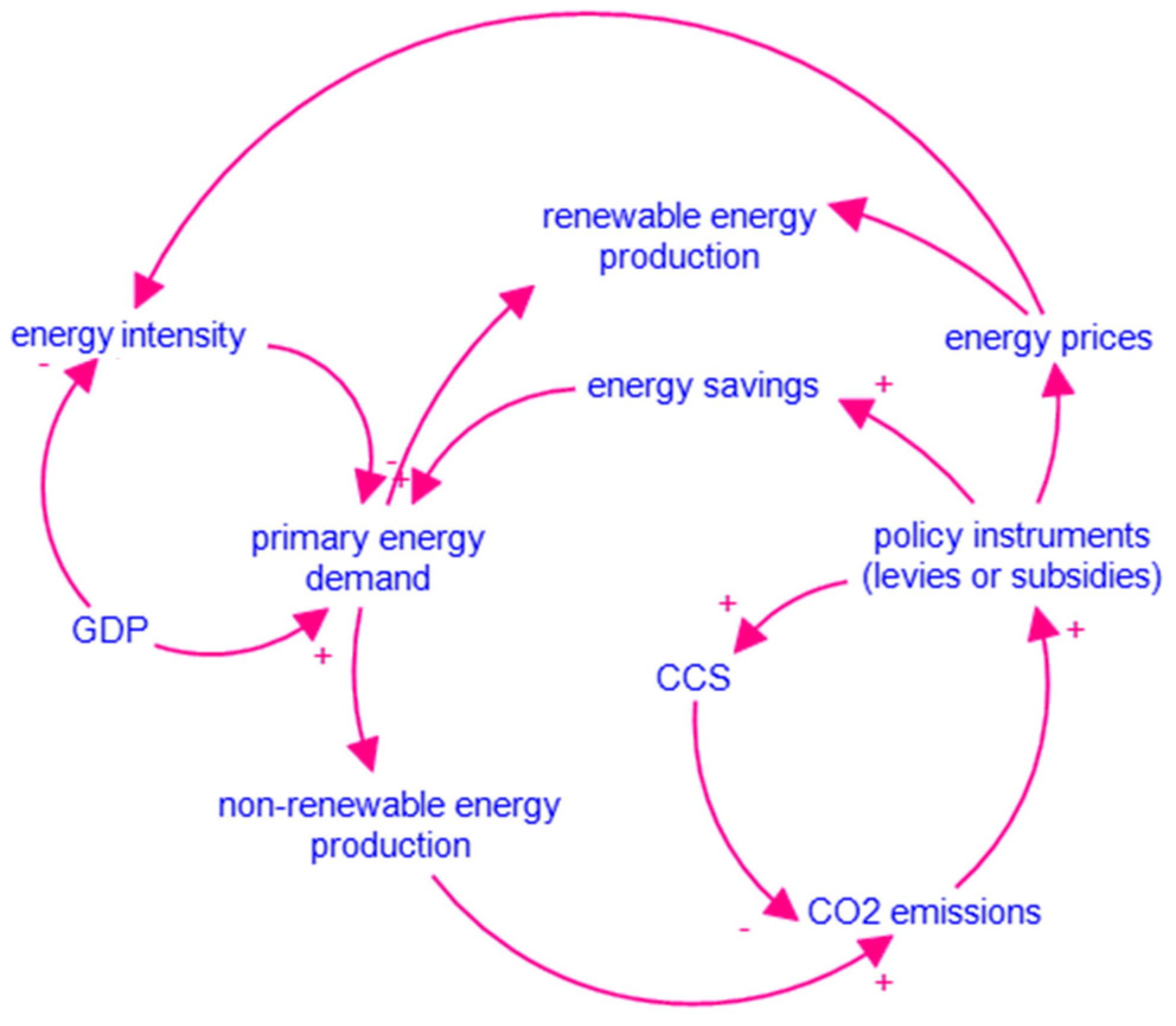
To assess mitigation options for reducing GHG emissions for achieving a low-carbon economy in the Netherlands, we developed the system dynamics model for energy policy (SDMEP). It includes a demographic/economic sub-system including GDP, an energy sub-system including energy demand and renewable as well as total energy generation and environmental sub-system (carbon emissions). The model focuses on the simulation of different policy scenarios, covering carbon levies and subsidies for mitigation options. The level of detail is adjusted to this focal point of the analysis and the model is validated to the assumptions of the projections of the study of the European Commission [16] as much as possible. Figure 2 displays the causal-loop diagram (CLD) of the SDMEP model, which identifies the main indicators and their relationships. A plus (+) in the CLD and indicates a positive relationship meaning that it if an indicator changes, the related indicator will change in the same direction. If the relationship is negative, a change in one variable causes the other variable to change in the opposite direction. When there is no polarity sign presented, the connector reflects either a negative or a positive relation.
The key indicator is the primary energy demand (PED) which is affected by the Gross Domestic Product (GDP) and energy intensity per unit of GDP (i.e., energy per €). PED is made equal to renewable energy (RE) and non-renewable energy (NRE) production, where we assume that total demand for energy equals total supply. For convenience, we assume no energy losses in the energy transportation, and international transportation is not considered. Non-renewable energy produces CO2 emissions. By means of levies or subsidies, the government can intervene and impact either promote renewable energy (RE) production via energy prices, stimulate energy savings (ES) or CCS, i.e., the mitigation options. In the SDMEP, we implement that the budget for subsidies to stimulate investments in energy-saving techniques must come from revenues generating activities such as carbon levies for instance.
The next step in the SDM process is building the quantitative SDMEP in software program Stella Professional [35]. Stella is widely used by SD modelers for simulation purposes [33]. In contrast to more mathematically based simulation software, Stella provides a user-friendly interface to visually build an SDM from which the mathematical rules can be derived. This user interface of Stella conveniently facilitates the linkages between different systems in a complexity model, which can be used to communicate with researchers less familiar with mathematics of simulation models.
To understand stock flow diagrams, one must know the four building blocks of Stella: stocks, flows, convertors, and connectors. A stock represents the level of any variable, it can either be tangible (e.g., natural capital) or not (e.g., information) and accumulates over time. Flows are connected to stocks and display the inflows or outflows of a stock. Convertors are either values or parameters created by a combination of different information sources in SDMEP or exogenously determined values.
In Figure 3, the four building blocks including symbols are presented: demographic/economic sub-model, energy sub-model, environmental sub-model, and the policy instruments sub-model, which represents the government. Finally, the connecters link all building blocks, reflecting causality within the model [26,27]. SDMEP is divided into three sub-models: the demographic, the energy, and the environmental sub-model, since the creation of sub-models is a way to deal with complexities of systems [24]. Furthermore, five economic sectors are defined, households, industry and energy sector, agricultural sector, services sector, and the transport sector. Furthermore, the energy system includes two types of energy sources, renewable (RE) and non-renewable energy (NRE) sources. Note that we do not distinguish varies types of renewable energy types. The environmental system includes the greenhouse gas emissions from energy production mainly. Below, we will subsequently describe the indicators and relationships between indicators and how we quantified them.

3.1. Demographic Sub-Model

The key indicators in the socio-economic sub-model are household income (HH) and sectoral added values (AV), see Figure 3. The initial stock value of total household income is household income per capita multiplied by the total population (POP) in 2010. The change of the stock value of total household income over time is affected by the population growth rate and the per capita income growth rate. For each production sector (all sectors except the households), we consider the value added. Value added per sector evolves over time with a particular sector-specific growth rate. The absolute changes of total income and value added are calculated explicitly in the model, see Figure 3.
Total household income and value added affect the demand for energy. The higher total household income or value added, the higher the demand for energy from these economic sectors. Moreover, total household income and total value added of sectors also affect the energy intensity of economic sectors.
Data for the Netherlands from 2010 to 2050 regarding GDP (including sectoral value added and household income) and population are taken from the 2015 Ageing Report [36]. The initial stock values for the aforementioned variables are values for 2010, since this is the base year of SDMEP, see Table 1. All monetary values were recalculated to 2010 values based upon the Consumer Price Index for the Netherlands. Additionally, the growth rates associated to the stocks differ across decades; thus, in total four growth rates are obtained from the 2015 Ageing Report, see Table 2.

3.2. Energy Sub-System

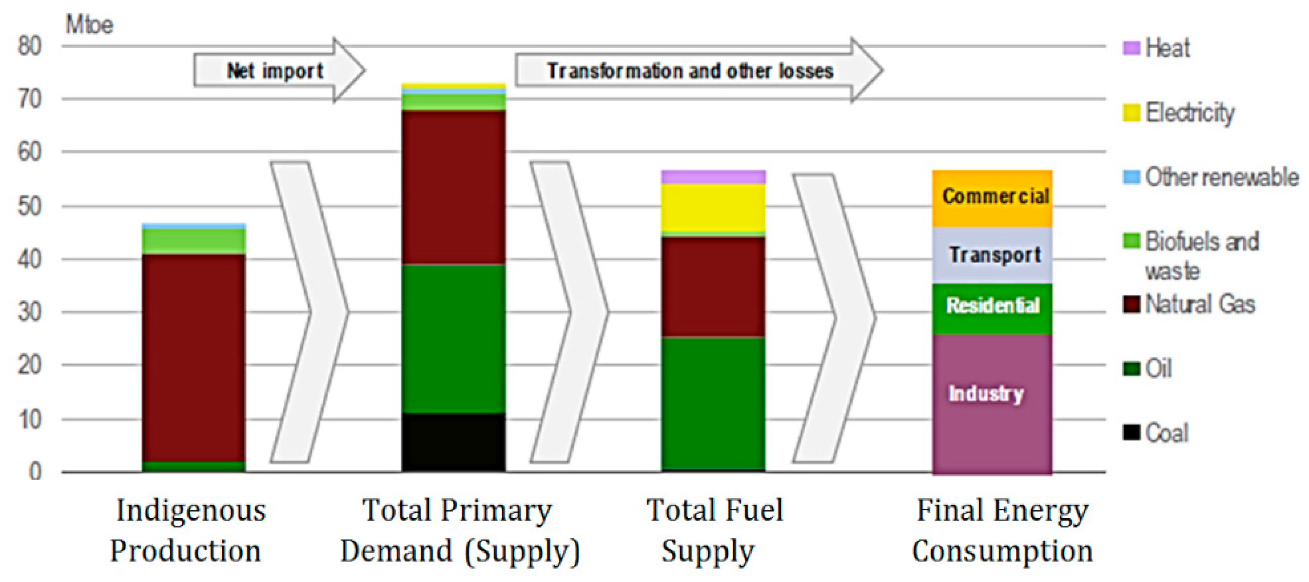
As mentioned above, SDMEP distinguishes two energy sources: renewable energy sources (RE) and non-renewable energy sources (NRE). RE are the energy sources that cannot be depleted by use; for example, heat sources (e.g., heat pump and geothermal heat), solar, wind, hydro, and bioenergy. NRE are fossil energy sources (i.e., oil, coal, and natural gas) and nuclear energy [14]. The change of the primary energy demand per year is influenced by the demographic indicators (household income and value added of economic sectors. The initial PED per year per group in 2010 in the Netherlands is obtained from the study of the European Commission [16], see Figure 4. PED consists of final energy consumption of end-users (i.e., all groups except for the energy sector) plus the energy demand from the energy sector itself (including transformation and distribution losses) and it excludes energy carriers for non-energy purposes [16], see Figure 4 for the composition of total primary energy demand and supply in the Netherlands in 2015.
Energy intensity is a stock on itself, whereby the initial stock values per group are determined by the model. The initial energy intensity growth rate per group is corrected for the effect of income and NRE prices on energy intensity development. The prices and income elasticities of NRE energy intensity over time were derived using energy intensity developments, income developments, and NRE prices. This is probably due to several other autonomous developments in the change of energy intensity over time assumed in the REF2016 scenarios [16]. The values of the parameters of the energy subsystem of SDMEP are determined in the calibration process based on the data from the business as usual (BaU) projections for PED in 2050, see Table 3.
When a subsidy for extra investing in energy-saving technologies is implemented, we assume that a certain amount of energy is subtracted from total energy demand. To convert subsidies for energy savings to actual energy saved, a conversion factor was needed which was calculated from the direct efficiency investment costs in Europe for additional energy savings compared to the baseline scenario [38]. The saving of 518 Mtoe extra energy would require 30 bn € annually; hence, 579 million € per ktoe per year, see Table 3.
Primary energy supply (PES) covers all energy needed for energy demands. PES includes primary energy production, net imports, bunkers, and stock changes. Recall that SDMEP distinguishes two types of energy namely RE and NRE. The initial RE production in the Netherlands is also obtained from [16], meaning that only renewable energy that is domestically produced, named primary energy production of renewables, is accounted for in the model. RE production abroad is not considered in SDMEP. Since the results of the energy production do not distinguish between renewable or non-renewable energy imports, we assume all imported energy is non-renewable energy [16]. It is important to realize that the Netherlands’ import dependency is expected to more than double in between 2010 (30%) and 2050 (69%). According to the REF2016 scenario of a study of the European Commission [16]. Consequently, the part of net imports that is produced as renewable energy is not accounted for in RE production in SDMEP.
To continue with RE production, RE production growth exists of two parts, whereof one is exogenous and obtained from the European Commission [16] as well, see Table 1.
Furthermore, RE production is influenced by fluctuations in prices of non-renewable energy prices as well as renewable energy prices. These prices solely exist of cost-prices and levies and/or subsidies. Cost-prices of NRE and RE were not given by the study of the European Commission [16] and therefore taken from [39] who used the PRIMES model. The cost price of NRE is an average of the pre-tax commodity prices for diesel oil, gasoline, fuel oil, kerosene, electricity, natural gas, naphtha, solids, and other liquids [39]. The average NRE price is based on a user-distribution in the Netherlands of 40% natural gas, 40% oil, and the rest coal. Price development from 2005 to 2050 were estimated in another study, where NRE prices are double in 2050 (from 498 € per ktoe energy in 2010 to 998 € per ktoe energy in 2050 [39].
The cost price of RE is an average of pre-tax commodity price of H2F and ethanol [39]; and levelized cost of CO2-neutral power generation [16]. “Levelized cost of electricity is net present value of unit-cost of electricity over the lifetime of a generating asset.” It serves as a proxy for the average price an asset must receive to be break-even over its lifetime. Initial investment, operations and maintenance, cost of fuel, cost of capital are included. [40]. The levelized cost of power generation of energy, i.e., the cost-price of CO2-neutral electricity, from 2010 to 2050 was obtained from the study of the European Commission [16]. These costs are based on weighted average cost of capital (WACC) of 7.5% real for annual capital cost and average operating hours per year as observed in 2016. The exact discount rate for each specific sector is given in the REF2016 report ([16], on average the discount rate for energy supply sectors is approximately 8%, for firms in demand sectors 9%, and for individuals in demand sector around 13%. In addition, RE generation technology is becoming less costly over the years; however, to what extent generation costs will decrease is highly uncertain. To illustrate, cost reductions ranging between 18 and 70% for CO2-neutral electricity technologies, and 20 and 40% for bioenergy technology between 2010 and 2100 [41]. The cost prices given showed a cost reduction of 38% from 2010 to 2050 [16,39].
Uncertainty also arises in future projections of fossil fuel prices. Several studies have tried to project the future price of fossil fuels and a large variation of such prices exists. To illustrate, a comparison of projected fossil fuel prices of different scenarios (e.g., The scenario study Welfare, Prosperity and the Human Environment (WLO) for the Netherlands and National Energy Outlook scenarios) [42]. Expectations regarding crude oil price ranges from 60 to 126 $/barrel in 2030 and from 74 to 149 $/barrel in 2050; such wide ranges also occur at future projections of the gas and coal price.
The effect of fluctuation of NRE and RE prices on the accumulation of RE production is captured in price elasticities. Price elasticities of specifically non-renewables and renewables were not given [16] and were non-existed for as far we know. A common price elasticity for energy demand is −0.2 to −0.3 and −0.7 for transport [14,43]; however, SDMEP requires a distinction between non-renewables and renewables; therefore, these common price elasticities cannot be used. For this reason, price elasticities are calculated with the use of data derived from the study of the European Commission [16]. Cost prices and energy production quantities are used to calculate the cross-price elasticity of NRE and the price elasticity of RE. The drawback of this approach is that other autonomous developments are included in the dynamic development of RE production, such as policies creating incentives, illustrating that production changes are not solely determined by changes in prices over time. As a result, elasticities are higher than expected, especially in the first ten to twenty years due to inclusion of policies in REF2016 projections. Cross price elasticities of NRE on RE production are in the first twenty years ranging between 4.6 and 2.3 in a decreasing fashion, subsequently going to a stable 0.7 for the last twenty years. RE price elasticities are particularly high and variable in the first twenty years (ranging from −8 to −2.30) and stable with a value of around −1.3 for the last twenty years. Note that the first 10 years of relatively high elasticities are not used in SDMEP because the model then fully runs on exogenous growth.
Another key point in the model is that we take the development of the ETS prices as given, and do not model the ETS price explicitly. There is assumed that the ETS price is determined at the European level. Under these circumstances, also the existing energy taxes of consumers would have to be implemented. Due to lack of clear overview of prices for different sectors and energy sources, we chose to include a uniform cost price per energy source. Consequently, the carbon levy in SDMEP is a national instrument on top of the value the ETS-prices and linked European price developments.

3.3. Environmental Sub-Model

Only energy-related CO2 emissions are considered in SDMEP. In particular, CO2 emissions from the energy branch and power generation: CO2 emissions from fossil fuels and biomass energy combustion, CO2 emissions through extraction of natural gas and oil, and CO2 emissions caused by transport and distribution of energy carriers; and all CO2 emissions that are released during the use and consumption of energy. CO2 emissions from non-energy uses, non-CO2 GHG emissions, and LULUCF are excluded. In SDMEP, there is no distinction between the autonomous growth rates of RE or NRE switch from different sectors, and thus regarding CO2 emissions.
Table 4 presents the carbon intensity of NRE production, which is a combination of carbon intensity of electricity and steam production; and final energy demand intensity which were given by the study of the European Commission [16]. Together with the share of electricity and steam production of total energy production, an average carbon intensity is calculated.
The CCS costs per tonne of CO2 were taken from a study of the Netherlands Environmental Assessment Agency (PBL) [14]. The value used, i.e., 50 € per tonne CO2, is an average of different CCS technologies where costs are ranging from 10 to 80 € per tonne CO2. CCS might also develop autonomously as a respond to a high enough carbon price, although expected to start around 2020–2025 [14,16]. Therefore, SDMEP includes a possibility to invest in CCS. Furthermore, carbon capture and utilization (CCU) is a fixed number per year and is not expected to grow in the short run [14].

3.4. Additional Assumptions

Electrification is accounted for in the exogenous growth of RE and is assumed to grow at a rate of 0.56% per year owing to the increase in electricity use for heating and cooling, increase of electric appliances in residential, agricultural and services sector [16]. Additionally, SDMEP assumes exchange rate from 1.12 $/€ in 2015 to 1.20 $/€ in 2025, at which is assumed to remain constant for the rest of the projection period [16].

3.5. Model Validation

After building SDMEP in Stella, the validity of the model is tested. Since we aimed to rebuild the assumptions of European reference scenarios [16] as much as possible, Table 4 therefore, compares BaU scenario results of SDMEP with REF2016 projections for 2050 [16]. In SDMEP, there are four economic sectors distinguished: agricultural sector (AR), service sector (SE), industry and energy sector (IE), transport sector (TR), and households (HH). Table 4 compares all endogenous determined stock values of SDMEP, i.e., total PED, individual PED of groups, energy intensity per group, total RE production and (energy related) CO2 produced per year to REF2016 projections. The base year values are also given. As one can see, the error margins are relatively small, i.e., all below 10%, except for PED of AR. This is due to aggregation of SE and AR under tertiary services while in SDMEP these sectors are separated [16]. A distribution of AR of tertiary services is only calculated in the start year and might change over the years but that is not factored in SDMEP. Nevertheless, if SE and AR were taken together in SDMEP similar to the study of the European Commission [16], the error margin would be 9.7%. Tertiary services in REF2016 projection demands 10452 ktoe of energy, and tertiary services in SDMEP 9433 ktoe, leading to 9.7% error margin. Under those circumstance, all error margins would be less than 10% and therefore we consider SDMEP is an acceptable model.
The REF2016 projection regarding energy intensity is based on exogenous growth rate of REF2016 [16] together with energy intensity in base year value that is calculated by total PED and HH income or sectoral added value).

4. Results

4.1. Scenarios

The aim of this study is to explore mitigation options that lead to a low-carbon economy in the Netherlands in 2050. We explore the impacts of three mitigations policy options with four policy scenarios using SDMEP. In all scenarios, a carbon tax is imposed to generate budget for the investments in mitigation options. All scenarios are budget neutral, i.e., revenues carbon tax equals spending on mitigation options. The first scenario stimulates the investments in bioenergy sources and CO2-neutral energy under renewable energy next to carbon levies (RE scenario). The second scenario stimulates investments in energy-saving options throughout the economy (ES scenario). The third policy option stimulates the investments in CCS to reduce greenhouse gas emission (CCS scenario). The mitigation option of electrifying the energy use (to abolish natural gas, coal, and other fossil fuel use), is autonomously included in all policy options considered. In order to observe the transition to a low-carbon economy, economics, energy, and the environment needed to be modelled, this requires an integration of different systems, simulated in integrated policy scenario (IP scenario). Fortunately, the SDM is able to cope with such integrations.

4.2. Business as Usual Scenario

SDMEP simulated that population in the Netherlands grew with 5% in 2050 relative to 2010. Before 2030, population is increasing to a peak level of almost 17.6 million people in 2030, henceforth slightly decreasing to 17.4 million people in 2050.
Total household income grew from 260 bn € to 483 bn € in 2050. The total added values doubles in 2050 to a level of 893 bn € whereof 515 bn € of services sector, 11 bn € of agricultural sector, 216 bn € of industry and energy sector, and 151 bn € of transport sector.
Furthermore, total PED in 2050 amounted 59,537 ktoe which is a decrease of 14% compared to PED in 2010. The share of RE production in total PED increased from approximately 5% in 2010 to 26% in 2050, see Table 5. The other 74% of PED, similar to 43,944 ktoe of NRE production, produces 113.7 MtCO2 in 2050, which is a CO2 reduction of 33% compared to 2010.

4.3. Policy Scenario Analysis

The aim of reducing CO2 with 80–95% as compared to 1990 is translated in the SDMEP as to reach, at least, the ultimate carbon target of 34 MtCO2 in 2050, by means of mitigations options supported by policy instruments. In total four policy scenarios, next to the BaU scenario, were run, whereof three scenarios capture the effects on mitigations options, and one aims to combine the mitigations options. The three mitigation options were identified as the most prominent mitigation options for achieving a low-carbon economy in the Netherlands in 2050 [14]. It was argued that a combination of mitigation options would be the most likely option, although a clear balance of options was not available. For the model results, it is important to realize is that policy instruments are implemented from year 2021 onwards due to already incorporated policies till 2020.
In Table 5, the simulation results for total PED, NRE production, RE production, CO2 emitted, and the values for carbon levy per ton CO2 and total subsidy over 30 years (2020 to 2050) are given. By means of iterative process, scenarios with carbon levies ranging from one to thirty € per ton of CO2 were run. The carbon levy amounts are inspired by calculations of an earlier study of CE Delft, which ran calculations on possible additional carbon levies above the ETS-price [42]. The run that was able to achieve the carbon target in 2050 with the lowest associated carbon levy is presented in Table 5. The results of the demographic economic sub-model are already described in the previous Section 4.1 and applies for the policy scenarios as well since population, household income, and added values stocks values were all exogenously determined.
Table 5 only displays the absolute values of the key variables in 2050. More detailed results over time are available upon request by the authors. A carbon levy of 4.75 € per ton CO2 generated in total 9.6 bn € of subsidies for supporting RE over the years 2020 to 2050. For the other two scenarios, i.e., CCS and ES policy scenarios, the carbon levy and total subsidy amount were almost double as high, see Figure 5. The fourth policy scenario aimed to compose the best combination of mitigation options in the Dutch economy. Simulations showed that a combination is not able to achieve the carbon target with a lower carbon levy than the RE policy scenario. Hence, the second-best scenario, integrated policy scenario, with a carbon levy of 5.30 € per ton and a subsidy amount 80% assigned to renewable energy (RE) and 10% assigned to energy saving (ES) and 10% to CCS.
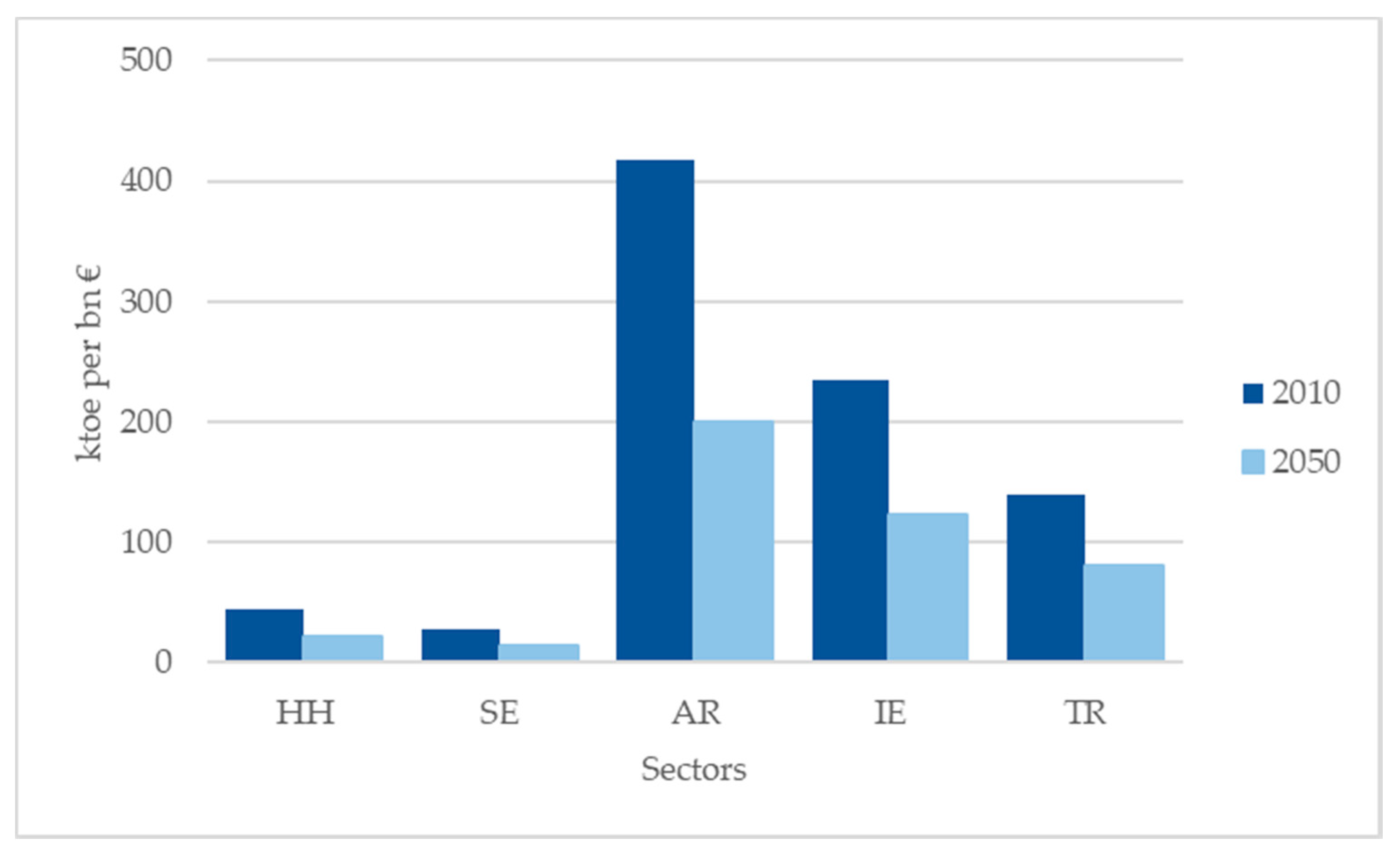
The energy intensities which are displayed in Figure 6. The initial values of energy intensities per groups in SDMEP were 44, 28, 418, 234, and 139 ktoe/bn € for households (HH), service sector (SE), agricultural sector (AR), industry and energy sector (IE) and transport sector (TR), respectively. Figure 6 shows the energy intensity per sector in the base year 2010 and in 2050 for the RE policy scenario, since this scenario had the lowest carbon levy. The other policy scenarios did not generate much different energy intensities per group as presented in Figure 6.
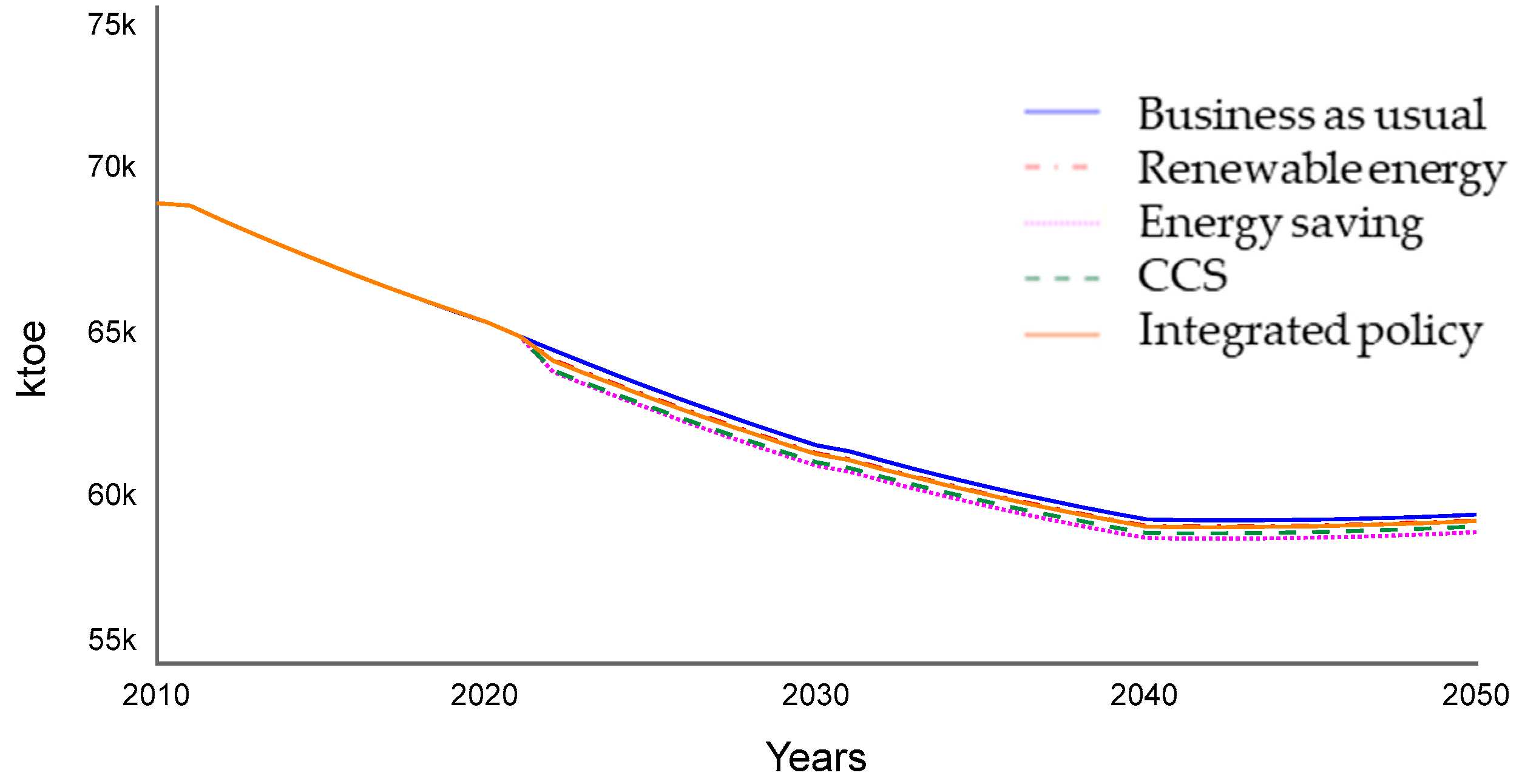
Total PED development under different policy scenarios can be seen in Figure 7. All scenario including the BaU scenario have 14% reduction of total PED in 2050 compared to 2010.
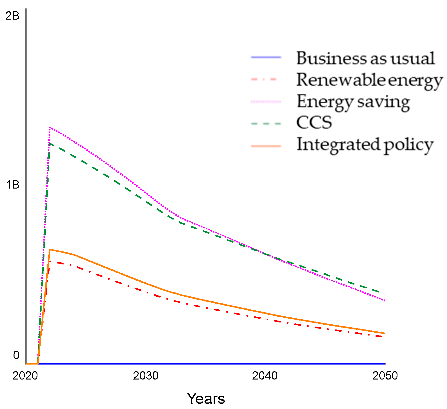
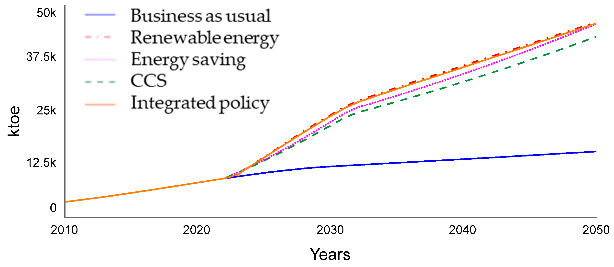
To continue, RE production increases the most under the RE policy scenario to a level of 46,190 ktoe in 2050, which is similar to 79% of total PED, as can be seen in Table 5. Immediately after 2020 RE production explodes in all policy scenarios, see Figure 8. In the end, RE production grows enormously under all policy scenarios, whereby under the RE policy scenario the most (approx. 1200%) and under the CCS policy scenario the lowest (approx. 1100%).
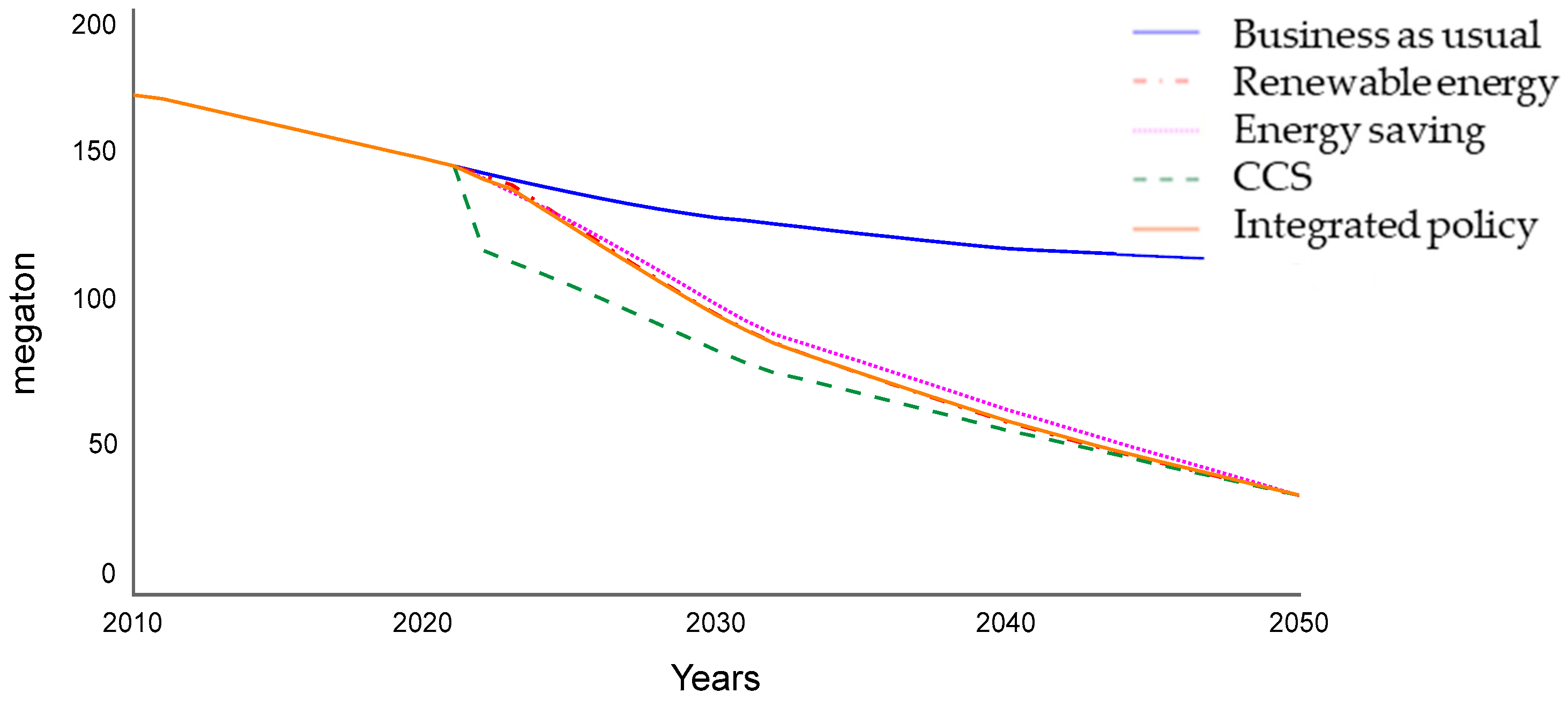
Figure 9 displays the development of CO2 released in atmosphere per year over the period 2010 to 2050.

4.4. Sensitivity Analysis

Parameters in SDMEP are subjected to a certain degree of uncertainty, so we tested the robustness of the model with varying the NRE price elasticity of energy intensity (NRE EI elasticity) and the income elasticity of energy intensity (Income EI elasticity). To explore the sensitivity of the aforementioned elasticities, a 25% range above and below the initial elasticity value is used. BaU scenario is then run again with one parameter change at the time, ceteris paribus. Since energy intensity is a determinant of PED, the total PED results in 2050 associated with different elasticities are given in Table 6. The values with an asterisk are the initial elasticity values. Between brackets are the percentage differences relative to the initial value, either elasticity or total PED, a positive value means an increase and a negative value a decrease towards the initial value. As one can see in Table 6, 25% increase in the NRE EI elasticity. leads to an increase of 5% in total PED, whereas a 25% decrease leads to a 4.5% reduction in total PED.
The total PED increase is just 1% as a result of a higher income EI elasticity and 0.8% reduction in case of a lower income EI elasticity (Table 7). Overall, SDMEP shows a weak sensitivity to NRE EI and income EI elasticity.
To check the robustness of simulation results with respect to key parameters, sensitivity analysis is performed on the cross and normal price elasticity of RE, and the conversion factors of ES and CCS. Table 7 presents the effect of different (cross) price elasticities values on total RE in 2050, ceteris paribus. The percentage between brackets reflects the change in comparison to the initial RE policy scenario results, indicated with asterisk. Furthermore, the row in italics presents the necessary adjustment of the height of the carbon levy to reach the carbon target again with changed price elasticities. Figure 10 displays the change in pathways of RE in case of lower elasticities. In particular, these lower elasticities are of interest because it brings the estimated price elasticities closer to price elasticities as described in the literature. As can be seen in Table 7, an increase (decrease) of one of the price elasticity lead to 7 to 10% increase (decrease) of total RE in 2050 and approximately 30% decrease (increase) of CO2 emissions in 2050. If both price elasticities are increased (decreased) the effect on total RE and CO2 emissions is twice the effect of changing one elasticity.
In addition, the sensitivity of conversion factors of ES and CCS regarding total energy savings and total CCS, respectively, is also tested (results in Table 8). Both conversion factors have a strong effect on their direct-linked mitigation option; however, a relatively weak effect on the annual CO2 emissions in 2050.

5. Discussion

The discussion on the BaU and four policy scenarios is structured as follows: Section 5.1 elaborates on key findings and Section 5.2 covers model uncertainties.

5.1. Key Findings

5.1.1. Renewable Energy Scenario versus Business-as-Usual Scenario

The energy intensities of sectors in the renewable energy (RE policy scenario) are halved compared to BaU scenario in 2050 (see Table 7). In other words, the number of energy units per € is significantly decreased. This is the result of either higher NRE energy prices, economic growth, or autonomous development of the overall efficiency level. Higher NRE energy prices might result in energy saving behavior of producers and consumers on the short-term and investment in clean and/or more efficient technologies in the long-term, leading to a downward effect on energy intensity. Economic growth leads to a lower energy intensity for example because of increased capacity to invest in new technology. A last part of this energy intensity improvement originates from autonomous improvement of the overall efficiency level [16].
The total primary energy demand (PED) in the RE policy scenario does not deviate much from the BaU scenario in 2050. This might be due to the relatively strong autonomous decline of total PED until 2050 in the BaU scenario. Another reason might be that policy instruments and mitigation options intended to reduce CO2 emissions, do not have a significant impact on total PED. In contrary to the energy mix, whereby the RE scenario results show a major shift from NRE to RE occurs in 2050 compared to the BaU scenario. This is illustrated by the 26% of renewables in the BaU scenario in 2050 to the almost 80% renewables in the RE policy scenario. This particular shift in the composition of the energy mix tends to be the main driver of CO2 emissions reduction. According to the BaU scenario, CO2 emissions would be still at a level of 113 MtCO2 per year in 2050, which is 70% more of emissions than the policy scenarios show in 2050.

5.1.2. Renewable Energy Scenario versus Other SDMEP Policy Scenarios

Despite that all policy scenarios reached the carbon target in 2050, they did not follow the same path towards that target. The RE policy scenario keeps the highest level of total PED, whereby one might expect higher CO2 emissions, but this effect is offset by the higher share of RE. The ES policy scenario shows, as expected, with 253 ktoe less energy in 2050 compared to the RE policy scenario, the lowest demand of energy. The CCS policy scenario has the second lowest PED and the integrated policy scenario thereafter. Moreover, the RE policy scenario has the highest share of RE compared to the other policy scenarios, which is a logical result when RE is subsidized. The CCS policy scenario, conversely, has the lowest RE share, which may reveal that the more carbon is captured and stored, the lower the need for RE, which was found in an earlier study as well [14]. All policy scenarios obtained relatively high shares of RE in 2050 (ranging between 72 and 79%), this is in line with expectations of previous studies [11,14,16]. Furthermore, CO2 emissions gradual decline towards 2050 in as well the RE policy scenario as in the ES policy and integrated policy scenarios, the CCS policy scenario, however, showed a more abrupt decline immediately after policy implementation in 2021 but eventually convergences to the other policy scenarios in the last decade (Figure 10). The abrupt decline of CO2 emissions of CCS can be explained by the relatively large availability of NRE in 2021 (still 91% of total PED), leading to a high government revenue to subsidize CCS, resulting in a large amount of CO2 captured and stored at once that year.

5.1.3. Degree of Government Intervention in SDMEP Policy Scenarios

Different levels of a carbon levy in each policy scenario are needed to enable economy to become low-carbon. This carbon levy are interpreted as an increase of the European ETS-price, starting from year 2021. Carbon levies in SDMEP are in the same range as earlier calculations of CE Delft [42], which also looked at an additional carbon tax above the ETS-price. However, they did not elaborate on the purpose of tax revenues such as the subsidies on RE, ES, or CCS, in contrast to this study. In this study the subsidies are always covered by additional tax revenues.
Simulation results (Table 7) show that in case of implementation of RE mitigation options a carbon levy of 4.75 € per ton of CO2, and a total subsidy amount of 9.6 bn € the carbon target in 2050 can be met. More steering of the Dutch government is necessary, indicated by the twice as high carbon levy compared to subsidizing RE, in order to achieve the carbon target with stimulating ES or CCS.
It is no surprise that the scenario with two policy instruments influencing the relative price of energy, i.e., increase of the NRE price (carbon levy) and decrease of the RE price (subsidy), is most effective. The ES and CCS policy scenarios only had the carbon levy to influence the relative price of energy, whereas the RE policy scenario that has two policy instruments, e.g., carbon levy per NRE unit and subsidy per RE unit influencing the relative energy price. Several studies [8,14,44,45] argued that such policy instruments are, among many others, one of the most effective policy instruments in stimulating an economy to reduce CO2 emissions. Such policy instrument affects the energy consumer/user directly and stimulates in this way, to opt for the greener source, in this case: renewable energy.
The main driving force behind CO2 emissions reduction is the implemented carbon levy and not per se the implementation of mitigation options in the Dutch economy. This follows from energy savings (ES) scenario results showing that only 40 ktoe is a direct result of support of the option energy saving. The rest of the declined energy demand in the ES scenario (compared to BaU) must, then, be induced by the implemented carbon levy. In case of the support of CCS, in total, i.e., an accumulation over 30 years, 434 MtCO2 is captured and stored. This is a considerable amount of CO2 stored; however, not yet close to reaching its potential (approximately 725 MtCO2) in the Netherlands given that a maximum of 25 MtCO2 can be stored in the North Sea each year [14]. A reason for the relatively limited contribution of ES and CCS to CO2 emissions reduction might be that implementation of ES and CCS is relatively costly compared to RE [14]. It is probably for this reason that the integrated policy scenario resulted in assigning 80% of total subsidy amount to subsidizing RE.
In practice, implementation of mitigation options might be harder than SDMEP outlines. Every mitigation option copes with challenges of implementation in the Dutch society. All scenarios show high shares of RE in 2050, in this study RE aggregated bioenergy and CO2-neutral electricity. To realize such RE shares, the Dutch have to rely heavily on the import of biomass [14], which is heavily debated and disputed from a sustainability perspective [46] due to the large GHG emissions when generating energy from biomass. Nevertheless, CO2-neutral electricity supply is expected not to be an issue in 2050, it is even projected that the Netherlands is going to export this particular electricity [15]. However, electrification is needed in order to exploit this Dutch CO2-neutral electricity. A major advantage of RE is that there is no major social resistance, mainly due to the many different existing types of renewables, this is in contrast to CCS. There is reasonable capacity in the Netherlands: in the North Sea and under main land; however, for now, no social acceptance exists regarding storage under main land [14]. The reason originates from the ignorance of the long-term effects of CO2 storage. Therefore, CCS is limited by the capacity in the North Sea, although the Dutch government may decide to store carbon abroad. To continue, the implementation of ES seems to be a complex one. On the one hand, ES are expected to develop due to improved energy efficient technologies [14], whereby extra government intervention tends to have less to nothing impact on the speed of such development, as indicated by our results. On the other hand, ES is often offset by other developments. To illustrate: incentives to save energy may vanish when the consumer or user already uses RE, or when energy efficiency improvement in for example electronic devices is offset by the increasing number of electronic devices per household (e.g., from maybe one computer per household to multiple laptops, phones, and tablets per household).

5.2. Model Uncertainties

This section aims to address model uncertainties divided into three types: uncertainty in model parameters, model drivers and model structure.
Firstly, many model parameters are subjected to a certain extent of uncertainty. The parameters in SDMEP are the (cross) price elasticity of RE, NRE EI elasticity, income EI elasticity, growth rates of EI of sectors, and the conversion factors of ES and CCS. On the calibrated parameters NRE EI elasticity and income EI elasticity the model showed a weak sensitivity given that a 25% change in either one of the elasticities, causes 1 to 5% change in total PED. However, a weak sensitivity of calibrated parameters may indicate that numerous values for these parameters are possible [47]. This was indeed the case in SDMEP. Furthermore, the estimated (cross) price elasticities used in SDMEP are relatively high compared to the normal energy demand elasticities found in the literature; however, they were of key importance for simulation results. Sensitivity analysis (Table 7) showed that changing price elasticities has a relatively small effect on their direct-linked variable, RE in this case, but at the same time, they pass on a relatively strong effect on final CO2 emissions. Additionally, the conversion factors of ES and CCS were tested. Conversion factors make it possible to convert subsidies to either an amount of energy saved, or an amount of CO2 captured and stored. In other words, it reflects the cost per unit of energy saved or per ton of CO2 captured and stored. The change in conversion factors did not lead to major changes in final CO2 emissions, despite the relatively strong effect on the level of implementation of mitigation options.
Secondly, model drivers form important pillars for SDMEP. Uncertainties mainly play a role at the demographic economic drivers of energy demand and energy prices as drivers for the energy mix. In SDMEP, demographic economic drivers are population, household income, and sectoral added value income. Regarding projection of population, several scenarios studies projected approximately the same population size in 2050; therefore, relatively little uncertainty is involved in this particular driver [13,14,16]. This is in contrast to economic drivers, as illustrated by the differences between the CPB and PBL study that distinguish low and high economic growth for the Netherlands [13] and the study of Fricko, which present five shared socioeconomic pathway (SSP) scenarios regarding economic activity in Europe [41].
Furthermore, to what extend economic activity drives the energy demand is subject to debate. Whereas earlier the energy demand used to grow with economic growth, studies now projects energy demand reduction together with economic growth (European Commission 2016a). Parameters reflecting the effect of economic activity on energy intensity and thus energy demand turned out to be small during calibrations in SDMEP, which is thus in line with the decoupling trend of economic activity and energy demand.
Moreover, energy prices are important drivers of the energy mix. As explained before, energy prices are highly uncertain in the future as can be concluded from the broad range of energy price estimations of different studies [12,14,41]. In addition, the complex international fuel market, the resource uncertainties, the unknown development of technologies make it hard to obtain reliable future energy price estimations [8]. Despite the different absolute energy price estimations, the dynamic development of NRE and RE prices tend to be more identical in different studies [16,39,41]. For this study, the dynamic development and the ratio of RE and NRE prices was more important than the absolute height of such prices.
On purpose some potential model drivers are left out in SDMEP, this is mainly due to avoid complexity in the model given the aim of this paper. SDMEP could be extended in two ways: energy prices as driver of economic growth and the effect of open borders within Europe on the energy mix. A connection from the energy sub-model to the demographic economic sub-model could have captured the effects of energy prices on economic growth and included the creation of green jobs. This would have closed the system, meaning that all key stock variables would have been endogenously determined. This could have led to for example a lower energy demand as a result of lower income as a reaction to higher energy prices.
The international character of the Netherlands is as well left out in SDMEP. This might have resulted in missing the effect of economies of scale or comparative advantages of countries in Europe. For example, solar energy in the South of Europe probably yields more electricity than in the North of Europe. Nevertheless, an advantage of modelling a closed economy was the prevention of carbon leakages.
The last source of uncertainty is the model structure. This study used an SD modelling approach out of the many modelling techniques that exists. Matter of course, each modelling technique has their advantages and disadvantages. In the light of system understanding, SD is a suitable approach. It is able to display how one change is passed on to the rest of economy, to detect (non-linear) behavior of system variables and to influence the system with time-dependent variables and time-delays. It gives in particular information about relationships and interdependencies of variables and sub-models. Additionally, it enables you to play with time; for example, implementation times of policies. To a certain extent, it is possible to include economical foundations such as finding the lowest carbon levy or working with the supply and demand market. However, SD is not an optimization model; therefore, prices must be endogenously modelled in SD. At last, feedback loops might not always be realistic [30].

6. Conclusions

This study aimed to address how a mix of climate mitigation options could be deployed in order to achieve a low-carbon economy. We applied SDMEP. For all scenarios, we considered as policy instruments a combination of a carbon levy and a subsidy on the mitigation options so that the subsidy is covered by the levy. The first research question was aimed to find insight in how mitigation options respond to policy instruments. Simulation results show that implementation of RE requires the lowest levies/subsidies compared to implementing ES and CCS. It is rather the carbon levy that enables the economy to go a low-carbon (e.g., energy savings) than the implementation of mitigation options. From our findings we aimed to see if there exist a combination of mitigation options that overrules the effectiveness of the dominant RE policy scenario. Since previous studies argued that all mitigation options are essential in reaching a low-carbon economy in 2050 [12,14]. The simulation results of the integrated policy scenario could not exceed the strong effect of implementation of solely RE. This raises the question whether indeed all mitigation options are needed as suggested by the earlier studies. Then again, their studies did not include an additional carbon levy, or elaborated on the financing of implementation of mitigation options. Imposing a carbon levy to finance subsidies to foster implementation of RE might be the better solution to reduce CO2 emissions than provide subsidies for—a combination of—mitigation options because their combined impact on emissions will be too limited. Especially since multiple studies confirmed, as this study as well, that implementation of ES and CCS is costly and difficult. Therefore, we would like to suggest for future energy policy, on the basis of these study results, to focus on establishing an additional carbon levy to the ETS-price. The budget raised could be used to subsidize the implementation of RE.
At last, future research regarding the specific price elasticities of RE and NRE could be of great interest of economic-energy models which aim to address the energy transition. Additionally, it would be interesting to look how the implementation of electrification can be supported by means of policy instruments.
For the Netherlands, there are additional issues to consider. First, a significant part of the greenhouse gas emissions are other types of greenhouse gas emission, such as methane (CH4) and nitrogen oxide (N2O). The required levels of greenhouse gas emissions for a low-carbon economy in the Netherlands urges to reduce those non-carbon GHG emissions as well. Second, land is already scarce in the Netherlands implying competing claims. The implementation of renewable energy options—whether or not it is energy from domestically produced biomass, solar power, or wind power—at a significant scale will have significant land requirements. These aspects need to be considered as well in future models.

Author Contributions

Conceptualization, V.L., K.D., and N.P.; methodology, V.L. and K.D.; software, K.D.; validation, K.D. and V.L.; writing—original draft preparation, V.L.; writing—review and editing, V.L., K.D., and N.P.; supervision, V.L. All authors have read and agreed to the published version of the manuscript.

Funding

The work described in this paper was conducted within the project SIM4NEXUS. This project received funding from the European Union’s Horizon 2020 research and innovation programme under Grant Agreement No 689150 SIM4NEXUS. This paper and the content included in it do not represent the opinion of the European Union, and the European Union is not responsible for any use that might be made of its content.

Acknowledgments

The authors thank Janez Sušnik and Sara Masia for their assistance with the Stella software.

Conflicts of Interest

The authors declare no conflict of interest.

References

  1. UNFCC The Paris Agreement. Report of the Conference of the Parties on its Twenty-First Session, Held in Paris from 30 November to 11 December 2015; UNFCC: Paris, France, 2015. [Google Scholar]
  2. Knutti, R. Relationship between global emissions and global temperature rise. In Climate Change 2013: The Physical Science Basis; Working Group I contribution to the IPCC Fifth Assessment Report; IPCC: Geneva, Switzerland, 2013. [Google Scholar]
  3. Allen, M.R.; Dube, O.P.; Solecki, W.; Aragón-Durand, F.; Cramer, W.; Humphreys, S.; Kainuma, M.; Kala, J.; Mahowald, N.; Mulugetta, Y.; et al. Framing and Context. In Global Warming of 1.5 °C. An IPCC Special Report on the Impacts of Global Warming of 1.5 °C Above Pre-industrial Levels and Related Global Greenhouse Gas Emission Pathways, in the Context of Strengthening the Global Response to the Threat of Climate Change, Sustainable Development, and Efforts to Eradicate Poverty; Masson-Delmotte, V., Zhai, P., Pörtner, H.-O., Roberts, D., Skea, J., Shukla, P.R., Pirani, A., Moufouma-Okia, W., Péan, C., Pidcock, R., et al., Eds.; The Intergovernmetnal Panel on Climate Change (IPCC): Geneva, Switzerland, 2018; p. 46. [Google Scholar]
  4. Ministerie van Economische Zaken. Energie Agenda: Naar een CO2 Arme Energievoorziening; Ministerie van Economische Zaken: Den Haag, The Netherlands, 2016; p. 120.
  5. CLO. Greenhouse gas emissions 1990–2015. Available online: www.clo.nl (accessed on 23 July 2017).
  6. ECN; PBL. Nationale Energieverkenning 2015; PBL: Den Haag, The Netherlands, 2015. [Google Scholar]
  7. CLO. Greenhouse gas emissions 1990–2019. Available online: https://www.clo.nl/indicatoren/nl0165-broeikasgasemissies-in-nederland (accessed on 12 July 2020).
  8. OECD Environmental Outlook to 2050: [The Consequences of Inaction]; OECD: Paris, France, 2012; ISBN 978-92-64-12224-6.
  9. WEC. World Energy Scenarios: Composing Energy Future to 2050; WEC: London, UK, 2013. [Google Scholar]
  10. Shell International Limited (SI). A Better Life with a Healthy Planet: Pathways to Net-Zero Emissions; Shell International Limited: London, UK, 2016. [Google Scholar]
  11. European Commission (Ed.) Energy Roadmap 2050; Energy; Publications Office of the European Union: Luxembourg, 2012; ISBN 978-92-79-21798-2. [Google Scholar]
  12. Ros, J.; Koelemeijer, R.; Elzenga, H.; Peters, J.; Hekkenberg, M. Towards a Clean Economy in 2050. An Outline of Roads. How the Netherlands can Become Climate-Neutral; (No. PBL--500083014); Planbureau voor de Leefomgeving PBL: The Hague, The Netherlands, 2011. [Google Scholar]
  13. CPB; PBL. Toekomstverkenning Welvaart en Leefomgeving; PBL: Den Haag, The Netherlands, 2015. [Google Scholar]
  14. PBL. Opties Voor Energie- en Klimaatbeleid; PBL: Den Haag, The Netherlands, 2016. [Google Scholar]
  15. European Commission. Energy Union and Climate Action: Driving EU’s Transition to a Low-carbon Economy; European Commission: Luxembourg, 2016. [Google Scholar]
  16. European Commission. EU Reference Scenario: Energy, Transport and GHG Emissions: Trends to 2050; European Commission: Luxembourg, 2016. [Google Scholar]
  17. Brouwer, F.; Vamvakeridou-Lyroudia, L.; Alexandri, E.; Bremere, I.; Griffey, M.; Linderhof, V. The Nexus Concept Integrating Energy and Resource Efficiency for Policy Assessments: A Comparative Approach from Three Cases. Sustainability 2018, 10, 4860. [Google Scholar] [CrossRef] [Green Version]
  18. Dekkers, K. Policy Instruments on Mitigation Options for a Low-carbon Economy in the Netherlands in 2050. Master’s Thesis, Wageningen University and Wageningen Economic Research, Wageningen, The Netherlands, 2017. [Google Scholar]
  19. Forrester, J.W. Industrial Dynamics; MIT Press: Cambridge, MA, USA, 1961; Volume 1, pp. 1–464. [Google Scholar]
  20. Jackson, M.C.; Keys, P. Towards a System of Systems Methodologies. J. Oper. Res. Soc. 1984, 35, 473–486. [Google Scholar] [CrossRef]
  21. Simonovic, S.P. World water dynamics: Global modeling of water resources. J. Environ. Manag. 2002, 66, 249–267. [Google Scholar] [CrossRef]
  22. Sušnik, J.; Molina, J.-L.; Vamvakeridou-Lyroudia, L.S.; Savić, D.A.; Kapelan, Z. Comparative analysis of system dynamics and object-oriented bayesian networks modelling for water systems management. Water Resour. Manag. 2013, 27, 819–841. [Google Scholar] [CrossRef]
  23. Naill, R.F. A system dynamics model for national energy policy planning. Syst. Dyn. Rev. 1992, 8, 1–19. [Google Scholar] [CrossRef]
  24. Dyner, I.; Smith, R.A.; Peña, G.E. System Dynamics Modelling for Residential Energy Efficiency Analysis and Management. J. Oper. Res. Soc. 1995, 46, 1163–1173. [Google Scholar] [CrossRef]
  25. Kibira, D.; Shao, G.; Nowak, S. Publications, Agencies and Staff of the U.S. Department of Commerce; U.S. Department of Commerce: Washington, DC, USA, 2010.
  26. Ahmad, S.; Mat Tahar, R.; Muhammad-Sukki, F.; Munir, A.B.; Abdul Rahim, R. Application of system dynamics approach in electricity sector modelling: A review. Renew. Sustain. Energy Rev. 2016, 56, 29–37. [Google Scholar] [CrossRef]
  27. Ford, A. Modeling the Environment, 2nd ed.; Island Press: Washington, DC, USA, 2010; ISBN 978-1-59726-472-3. [Google Scholar]
  28. Bolwig, S.; Bazbauers, G.; Klitkou, A.; Lund, P.D.; Blumberga, A.; Gravelsins, A.; Blumberga, D. Review of modelling energy transitions pathways with application to energy system flexibility. Renew. Sustain. Energy Rev. 2019, 101, 440–452. [Google Scholar] [CrossRef]
  29. Roberts, N.; Andersen, D.F.; Deal, R.M.; Garet, M.S.; Shaffer, W.A. Introduction to Computer Simulation: The System Dynamics Approach; Addison-Wesley Publishing Company: Boston, MA, USA, 1983; ISBN 0-201-06414-6. [Google Scholar]
  30. Kelly, R.A.; Jakeman, A.J.; Barreteau, O.; Borsuk, M.E.; ElSawah, S.; Hamilton, S.H.; Henriksen, H.J.; Kuikka, S.; Maier, H.R.; Rizzoli, A.E. Selecting among five common modelling approaches for integrated environmental assessment and management. Environ. Model. Softw. 2013, 47, 159–181. [Google Scholar] [CrossRef]
  31. Liu, X.; Mao, G.; Ren, J.; Li, R.Y.M.; Guo, J.; Zhang, L. How might China achieve its 2020 emissions target? A scenario analysis of energy consumption and CO2 emissions using the system dynamics model. J. Clean. Prod. 2015, 103, 401–410. [Google Scholar] [CrossRef]
  32. Xiao, B.; Niu, D.; Guo, X. Can China achieve its 2020 carbon intensity target? A scenario analysis based on system dynamics approach. Ecol. Indic. 2016, 71, 99–112. [Google Scholar] [CrossRef]
  33. Feng, Y.Y.; Chen, S.Q.; Zhang, L.X. System dynamics modeling for urban energy consumption and CO2 emissions: A case study of Beijing, China. Ecol. Model. 2013, 252, 44–52. [Google Scholar] [CrossRef]
  34. Ansari, N.; Seifi, A. A system dynamics model for analyzing energy consumption and CO2 emission in Iranian cement industry under various production and export scenarios. Energy Policy 2013, 58, 75–89. [Google Scholar] [CrossRef]
  35. Isee Systems. Available online: http://www.iseesystems.com (accessed on 12 July 2020).
  36. European Commission. The 2015 Ageing Report: Underlying Assumptions and Projection Methodologies; European Commission: Luxembourg, 2014. [Google Scholar]
  37. IEA. World Energy Outlook 2010; World Energy Outlook; OECD Publishing: Paris, France, 2010; ISBN 978-92-64-08624-1. [Google Scholar]
  38. European Commission. Proposal for Directive of the European Parliament and of the Council mending Directive 2012/27/EU on Energy Efficiency; European Commission: Brussels, Belgium, 2016. [Google Scholar]
  39. Capros, P. PRIMES Energy System Model: Overview of PRIMES Modelling Approach; E3MLab-National Technical University of Athens: Athens, Greece, 2010. [Google Scholar]
  40. Ueckerdt, F.; Hirth, L.; Luderer, G.; Edenhofer, O. System LCOE: What are the costs of variable renewables? Energy 2013, 63, 61–75. [Google Scholar] [CrossRef]
  41. Fricko, O.; Havlik, P.; Rogelj, J.; Klimont, Z.; Gusti, M.; Johnson, N.; Kolp, P.; Strubegger, M.; Valin, H.; Amann, M.; et al. The marker quantification of the Shared Socioeconomic Pathway 2: A middle-of-the-road scenario for the 21st century. Glob. Environ. Chang. 2017, 42, 251–267. [Google Scholar] [CrossRef] [Green Version]
  42. CE Delft. Kosteneffectiviteit Van Maatregelen Voor CO2-Reductie in Nederland; CE Delft: Delft, The Netherlands, 2017. [Google Scholar]
  43. CE Delft. Economische Ontwikkelingen Energie-Intensieve Sectoren; CE Delft: Delft, The Netherlands, 2014. [Google Scholar]
  44. Snyder, L.D.; Miller, N.H.; Stavins, R.N. The Effects of Environmental Regulation on Technology Diffusion: The Case of Chlorine Manufacturing. Am. Econ. Rev. 2003, 93, 431–435. [Google Scholar] [CrossRef] [Green Version]
  45. Bailey, I. Market Environmentalism, New Environmental Policy Instruments, and Climate Policy inthe United Kingdom and Germany. Ann. Assoc. Am. Geogr. 2007, 97, 530–550. [Google Scholar] [CrossRef]
  46. SER. Biomassa in Balans: Een Duurzaamheidskader Voor Hoogwaardige Inzet Van Biogrondstoffen; Sociaal Economische Raad/Economic and Social Council (SER): Den Haag, The Netherlands, 2020; p. 113. [Google Scholar]
  47. Pianosi, F.; Beven, K.; Freer, J.; Hall, J.W.; Rougier, J.; Stephenson, D.B.; Wagener, T. Sensitivity analysis of environmental models: A systematic review with practical workflow. Environ. Model. Softw. 2016, 79, 214–232. [Google Scholar] [CrossRef]
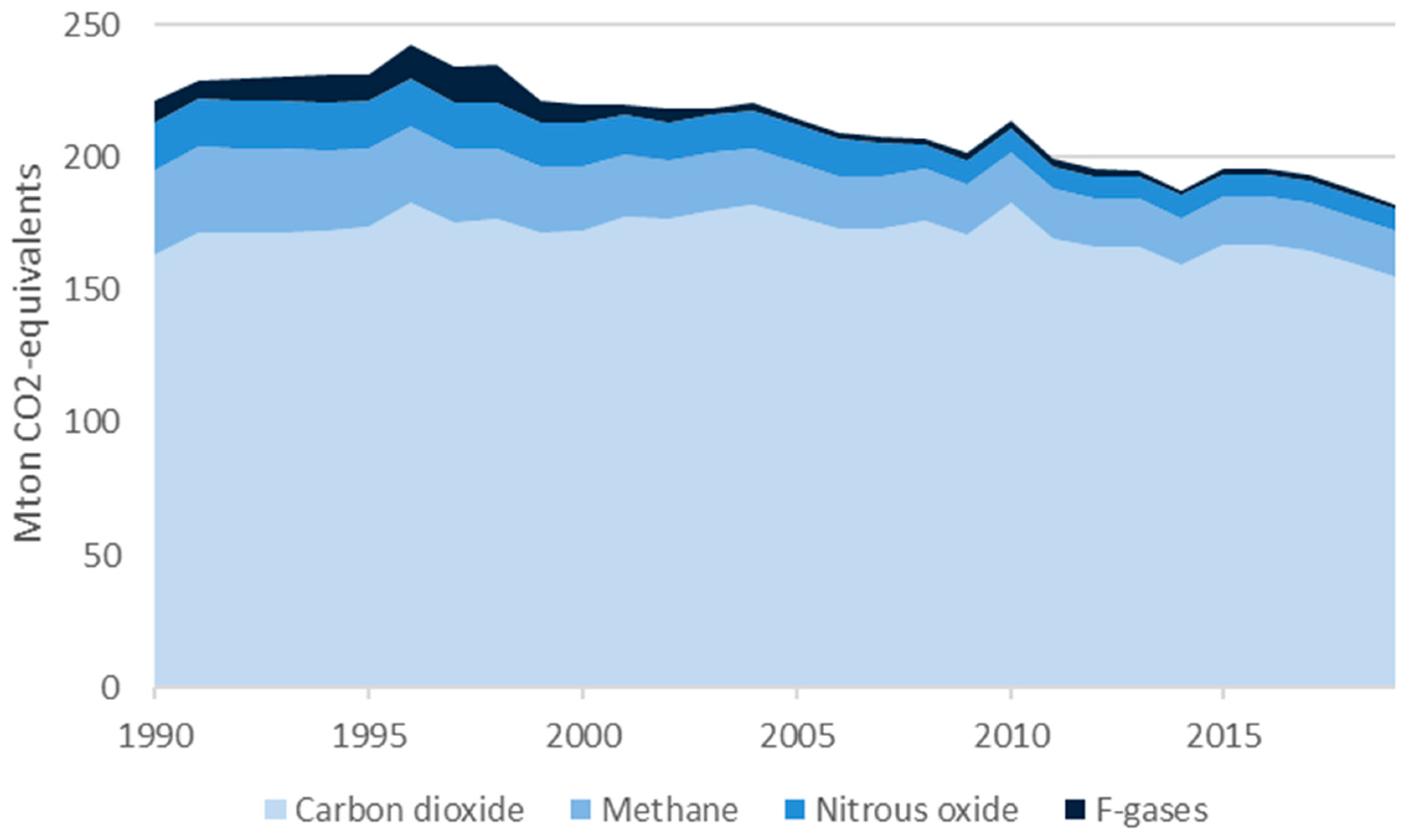
Figure 1. Greenhouse gas emissions development in the Netherlands 1990–2019. Derived from [7].
Climate 08 00132 g001
Figure 2. Causal Loop Diagram of System Dynamics Model for Energy Policy (SDMEP).
Climate 08 00132 g002
Figure 3. Scheme of the System Dynamics Model for Energy Policy in Stella software.
Climate 08 00132 g003
Figure 4. Explanation of energy demand and supply, own calculation based upon [37].
Climate 08 00132 g004
Figure 5. Total subsidy amount (€) 2020–2050.
Climate 08 00132 g005
Figure 6. Energy intensities (ktoe/bn €) per group in the Renewable Energy (RE) policy scenario in 2050.
Climate 08 00132 g006
Figure 7. Total primary energy demand per year 2010–2050.
Climate 08 00132 g007
Figure 8. Total renewable energy per year 2010–2050.
Climate 08 00132 g008
Figure 9. Total CO2 released per year 2010–2050
Climate 08 00132 g009
Figure 10. Total renewables subjected to different (cross) price elasticities.
Climate 08 00132 g010
Table 1. Initial stock values (price level = 2010) for the demographic sub-system.
Initial Stock Values Unit *Initial ValueSource
Household income per capita (HH income)15,735[36]
Population (POP)mln 16.6[36]
Added value services sector (SE)bn €333 [36]
Added value agricultural sector (AR)bn €10.6[36]
Added value industry and energy (IE)bn €136.8[36]
Added value transport (TR)bn €114.6[36]
Primary energy demand per year (HH)ktoe11,518.4[16]
Primary energy demand per year (SE)ktoe8822.0[16]
Primary energy demand per year (AR)ktoe4302.0[16]
Primary energy demand per year (IE)ktoe29,402.3[16]
Primary energy demand per year (TR)ktoe14,984.7[16]
Initial CCSktoe0[14]
* bn is billion, mln is million, ktoe is kilo tonne of oil equivalent.
Table 2. Annual exogenous growth rates of group incomes, population [36], and renewable energy production in the Netherlands [16].
Growth Rates2010–20202020–20302030–20402040–2050Source
Household income growth rate0.7%1.1%1.5%0.19%[36]
Population growth rate0.3%0.2%−0.05%−0.05%[36]
Growth rates of value added per sector
Services sector0.8%1.1%1.4%1.6%[36]
Agricultural sector1.1%0.6%−0.2%0.1%[36]
Industry and energy sector1.2%0.8%1.3%2.2%[36]
Transport sector0.8%0.9%1.1%0.5%[36]
Renewable energy primary production10.5%1.4%1.2%1.2%[16]
Table 3. Parameter values of the energy sub-system.
Parameter Values Initial ValueSource
Energy intensity growth rate (HH)−0.0012Calibrated
Energy intensity growth rate (SE)−0.0012Calibrated
Energy intensity growth rate (AR)−0.0133Calibrated
Energy intensity growth rate (IE)−0.0078Calibrated
Energy intensity growth rate (TR)−0.01Calibrated
Energy intensity elasticity of income−0.0816Calibrated
Energy intensity elasticity of non-renewable energy (NRE) prices−0.281Calibrated
Carbon intensity (MtCO2/ktoe)0.002655[16]
Direct energy efficiency investment cost per ktoe (mln €) 579[38]
Costs CCS per MtCO2 (mln €/MtCO2) 50[14]
CCU (ktoe) 3[14]
Table 4. Model validation results.
Key Energy IndicatorsBase YearProjection
REF2016BaUError Margin
20102050
Energy Intensity (ktoe/bn €)
Households (HH)
Service sector (SE)
Agricultural sector (AR)
Industry and energy sector (IE)
Transport sector (TR)

44
28
418
234
139

23
14
202
131
88

21.3
13.7
200.3
123.3
81.4

7.4%
0.7%
0.8%
5.9%
7.5%
Total primary energy demand( PED) (ktoe)
Households (HH)
Service sector (SE)
Agricultural sector (AR)
Industry and energy sector (IE)
Transport sector (TR)
69,030
11,518
8822
4302
29,402
14,985
59,530
10,645
7026
3426
24,790
13,643
59,537
10,554
7189
2244
27,104
12,446
0.0%
0.1%
2.3%
34.5%
9.3%
8.8%
RE production (ktoe)367114,47315,5947.7%
CO2 emissions released per year (MtCO2)1751121141.8%
Table 5. Simulation results effect policy instruments and mitigations options on primary energy demand (PED) and energy mix in 2050 (* accumulated over 2021 to 2050).
Key Energy Indicators.Mitigation OptionsPolicy Instruments
Scenarios Average Energy Intensity (ktoe/€) Primary Energy Demand (ktoe)Share RE of Total PED (%) Renewable Energy Production (ktoe) Accumulated * Energy Savings (ktoe)Accumulated * CCS
(MtCO2)
Carbon Levy per ton CO2 (€)Accumulated * Subsidy Amount (€ bn)
1. BaU 172.659,53826.215,594----
2. RE policy87.859,37078.846,190--4.759.6
3. ES policy87.459,11777.845,9934043411.0022.8
4. CCS policy87.559,18272.242,751--10.2022.1
5. Integrated policy 87.859,34977.445,9102215.3010.7
* This is the sum of annual values of the indicator for the period 2020–2050.
Table 6. Sensitivity of non-renewable energy (NRE) energy intensity (EI) elasticity and income EI elasticity on total PED.
Impact NRE EI Elasticity.Impact Income EI Elasticity
Change of ElasticitiesNRE EI
Elasticity
Total PED (Mtoe)Income EI ElasticityTotal PED (Mtoe)
Initial−0.281059.5−0.081659.5
−25%−0.2110 (+25%)62.4 (+5%) −0.0612 (+25%)60.1 (+1%)
+25%−0.3510 (−25%)56.8 (−4.5%)−0.1020 (−25%)59.0 (−0.8%)
Table 7. Sensitivity analysis price elasticities (* is initial simulation result of CL RE scenario).
Price ElasticitiesTotal RE (Mtoe) in 2050 Annual CO2 Emissions (Mt) in 2050Carbon Levy (€ per ton CO2)
Cross Elasticity.Normal Elasticity.
**46.2 *34 *4.75 *
+25%-+7.8%−27.6%
-+25%+9.1%−31.5%
+25%+25%+17.1%−58.8%
+25% +25%0.0%0.0%-20%
−25%-−7.4%+23.5%
-−25%−10.0%+32.4%
−25%−25%−16.9%+55.9%
−25%−25%0.0%0.0%+33%
Table 8. Sensitivity analysis on conversion factor ES.
Energy Saving (ES) ScenarioCCS Scenario
Change in CONVERSION FactorConversion Factor ES (mln €)Accumulated Energy Savings (ktoe)Annual CO2 Emissions (Mt) in 2050Conversion Factor CCS (mln €)Accumulated CCS (MtCO2) Annual CO2 Emissions (Mt) in 2050
Initial579 *40 *34 *50 *434 *34 *
−25%−25%+30%−0.03%−25%+33.2%−7.9%
+25%+25%−82.5%0.00%+25%−20%+4.4%
* is initial simulation result of the CL ES scenario. Energy savings are accumulated over the entire time period, in contrast to CO2 emissions which is an amount per year in 2050.
Publisher’s Note: MDPI stays neutral with regard to jurisdictional claims in published maps and institutional affiliations.