Article

Observed Mesoscale Hydroclimate Variability of North America’s Allegheny Mountains at 40.2° N

1
Institute of Water Security and Science, West Virginia University, Agricultural Sciences Building, Morgantown, WV 26506, USA
2
Davis College, Schools of Agriculture and Food, and Natural Resources, West Virginia University, 3109 Agricultural Sciences Building, Morgantown, WV 26506, USA
*
Authors to whom correspondence should be addressed.
Climate 2019, 7(7), 91; https://doi.org/10.3390/cli7070091
Submission received: 3 June 2019 / Revised: 6 July 2019 / Accepted: 6 July 2019 / Published: 18 July 2019
(This article belongs to the Special Issue Landscape and Climate Change)

Abstract

:
Spatial hydroclimatic variability of Eastern North America’s Allegheny Mountain System (AMS) is commonly oversimplified to elevation differences and the rain-shadow effect. Descriptive and higher order statistical properties of hourly meteorological observations (1948–2017) from seven airports were analyzed to better understand AMS climatic complexity. Airports were located along a longitudinal transect (40.2 °N) and observation infrastructure was positioned to minimize climatic gradients associated with insolation, slope, and aspect. Results indicated average ambient temperature was well correlated with airport elevation (R2 = 0.97). However, elevation was relatively poorly correlated to dew point temperature (R2 = 0.80) and vapor pressure deficit (R2 = 0.61) heterogeneity. Skewness and kurtosis of ambient and dew point temperatures were negative at all airports indicating hourly values below the median were more common and extreme values were less common than a normal distribution implies. Westerly winds accounted for 54.5% of observations indicating prevailing winds misrepresented nearly half of AMS weather phenomena. The sum of maximum hourly precipitation rates was maximized in Philadelphia, PA implying a convective precipitation maximum near the border of Piedmont and Coastal Plain provinces. Results further indicate the AMS represents a barrier to omnidirectional moisture advection suggesting physiographic provinces are characterized by distinct evapotranspiration and precipitation regimes. The current work draws attention to observed mesoscale hydroclimatic heterogeneity of the AMS region and identifies mechanisms influencing local to regional water quantity and quality issues that are relevant to many locations globally.

Graphical Abstract

1. Introduction

Spatial hydroclimatic variability of Eastern North America’s Allegheny Mountain System (AMS) is often oversimplified by assumptions of elevation differences and the rain-shadow effect. The dimensions of topographic features [1], orientation relative to prevailing winds (e.g., Froude number; [2]), and the slope and the aspect [3] influence climatic variability across a range of spatiotemporal scales [4]. As a result, topographic features modulate coupled exchanges of energy (e.g., heat), mass (e.g., water), and momentum at the Earth-atmosphere interface. For example, adiabatic cooling and expansion of air currents ascending mountain slopes (i.e., upslope) often results in cloudiness, precipitation, and fog-water deposition that supplies water and reduces insolation [5,6,7]. Adiabatic warming and compression of air currents descending mountain slopes (i.e., downslope) reduces average humidity, cloud cover, and precipitation across regions often referred to as rain-shadows [8,9,10]. Ultimately, mountain barriers influence precipitation patterns by affecting where precipitation falls associated with storms (e.g., cyclones and convection) developing near or traversing mountainous terrain [9]. As a result, the geographic orientation of mountain barriers combined with elevation, slope, and aspect result in spatially complex gradients in fundamental atmospheric variables that directly influence ecological diversity.
Complex microclimatic heterogeneities inherent to North America’s Allegheny Mountain System (AMS) support some of the most ecologically diverse forests in the United States’ Forest System (e.g., Monongahela National Forest; [11]). Despite the AMS’s rich ecological diversity and spatial expanse (20° latitude by 30° longitude; [12]), climatic gradients perpendicular to the AMS are not well documented [13]. In 1959, elevation-dependent relationships between daily mean values of temperature, potential evapotranspiration, and growing-season length were quantified within the southern AMS [14]. However, latitudinal bioclimatic gradients resulting from insolation can confound elevation-dependent relationships in climatic variables [15]. Latitudinal insolation gradients are particularly relevant to the AMS that extends more than 2000 km from Newfoundland, Canada southwest into Alabama, USA [16]. For example, the bioclimatic threshold between coniferous and deciduous species within the AMS decreases from 1680 m at 35°N to 150m at 49°N (-100 m °latitude-1; [17]). Bioclimatic zonation of the AMS is influenced by high elevation cloud immersion that increases the proportion of diffuse insolation and substantially contributes to annual water inputs through canopy interception processes [6,18,19,20]. Furthermore, observed trends in cloud base heights implies latitudinal insolation gradients influenced cloud immersion frequency and resultant bioclimatic diversity as temperatures warmed [21,22]. Thus, climatic analyses that minimize gradients associated with latitude, slope, and aspect will improve understanding of microclimatic heterogeneity and associated bioclimatic diversity within the AMS and similar mountains regions, globally.
The AMS is a sub-region of Appalachia that is located south and west of New York State’s Hudson and Mohawk valleys [16]. The AMS’s geographic position within prevailing mid-latitude westerlies results in a succession of extratropical cyclones (ETC) that are responsible for many high-impact weather events including flooding [23,24]. In particular, Appalachia’s warm season thunderstorms result in some of the largest rainfall accumulations—measured anywhere on Earth—at time scales less than 6 h [25,26,27]. Short duration, high intensity precipitation characteristic of thunderstorms can result in flash flooding, debris flows, and landslides due to the steep slopes of Appalachia’s Allegheny and Blue Ridge Mountain Ranges [26]. Despite longitudinal gradients in heavy rainfall frequency [28], flash flooding can occur anywhere within or nearby the AMS [27] and climatic analyses based on observed data are especially lacking in the AMS. Additionally, vulnerabilities to flash flooding may be exacerbated by super Clausius-Clapeyron scaling [29] of an increasingly humid Allegheny climate [30] and may be compounded by wetter antecedent conditions [31] due to more frequent precipitation [32]. Quantitative understanding of longitudinal climatic gradients needs to be improved to prepare communities for the likelihood of more frequent and severe floods.
Hourly observations provide insights that more commonly utilized daily data cannot provide. For example, an analysis of higher order statistical moments (e.g., skewness and kurtosis; [33,34]) provides information on the probability distribution properties that are more robust with larger sample sizes. As a result, hourly meteorological terminal aviation routine (METAR) observations may be a suitable observation platform to better quantify mesoscale climatic variability within complex landscapes. METAR and automated surface observing systems (ASOS) were the primary observation codes used in the United States to satisfy requirements for reporting surface meteorological data documented in the Federal Meteorological Handbook [35]. Prior to the 1990s, METARs were recorded manually by certified observers and were subjected to a near real-time quality control program ensuring proper observational procedures and routine maintenance of instrumentation [35]. Increasing labor costs associated with manual weather observation at hundreds of airports across the United States spurred the development of ASOS in the 1980’s [36,37]. ASOS observations (1990s-present) reduce or eliminate direct human involvement in acquiring, processing, and disseminating surface observations. A standard ASOS consists of a ceilometer, a visibility sensor, a shielded and heated tipping bucket precipitation gauge, a cup anemometer at 10m, redundant digital pressure transducers, a platinum wire resistive temperature device, and a chilled mirror to measure dew point temperature [36,37]. All ASOS data are subjected to quality control algorithms at three temporal or spatial scales [36,37]. Importantly, federal standards for siting meteorological sensors attempted to minimize or eliminate microclimatic effects of manmade or geographical obstructions including the slope or the aspect [38]. Therefore, METAR observations are well-suited in identifying mesoscale (4 to 400 km; [39]) climatic gradients across the AMS’s rugged landscape.
The overarching objective of the current work was to quantify mesoscale climate heterogeneity using hourly observations at seven airports positioned across the Allegheny Mountains at approximately 40.2°N to minimize gradients associated with slope, aspect, and insolation. Sub-objectives included a) quantifying annual climatic oscillations relative to solstice and equinox dates, b) assessing mesoscale variability of higher order statistical properties of hourly temperature, humidity, and vapor pressure deficit (VPD) observations, and c) assessing spatial and temporal characteristics of precipitation regimes to improve upon the traditionally accepted rain-shadow hypothesis.

2. Materials and Methods

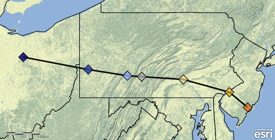
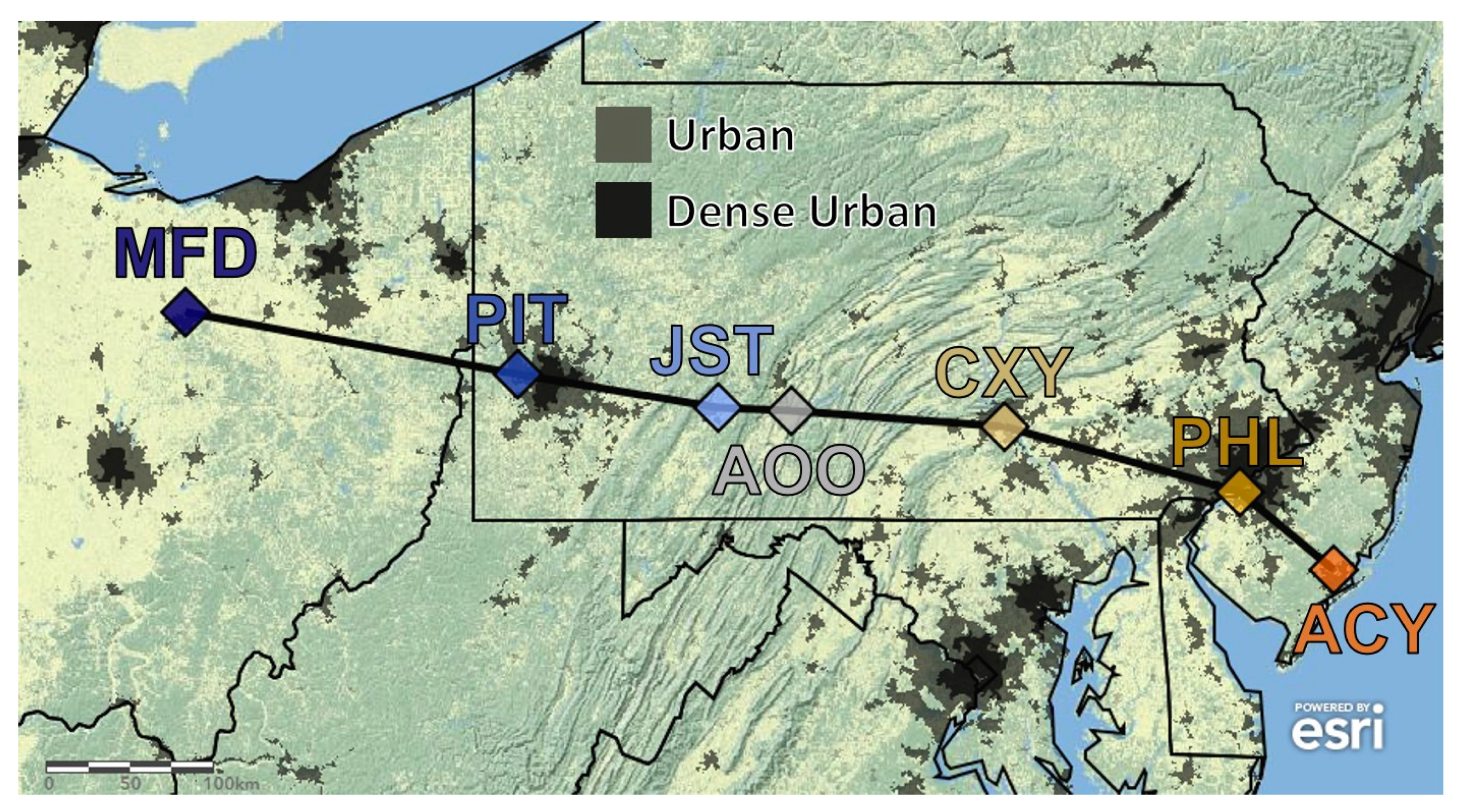
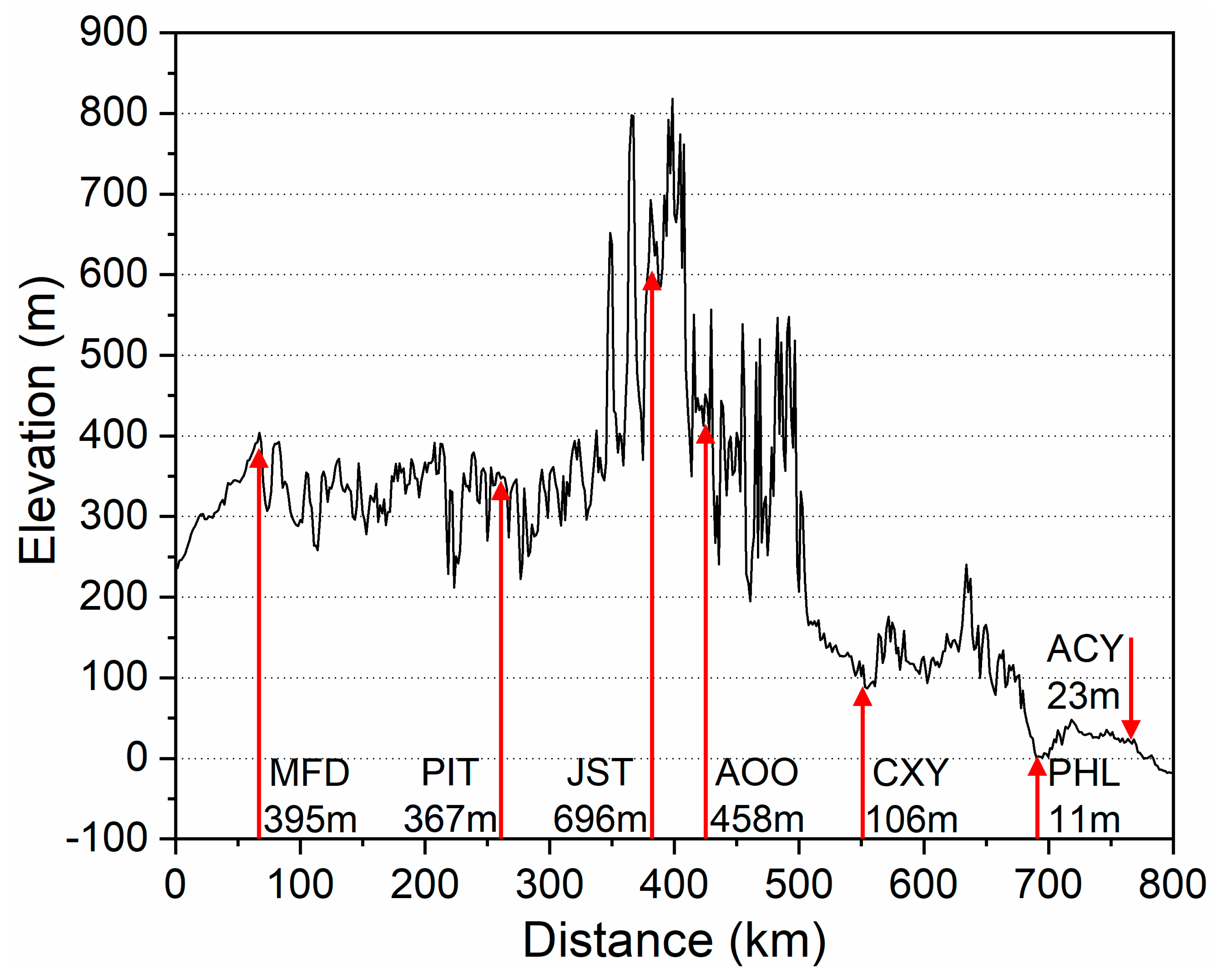
2.1. Transect Physiography

Airports in Pennsylvania (n = 5), Ohio (n = 1), and New Jersey (n = 1), USA were selected for the current work. From here forward the airports investigated in the current work are referred to as the cross Allegheny transect (CAT; Figure 1). From west-to-east, the seven airports were Mansfield Regional Airport (MFD), Pittsburgh International Airport (PIT), Johnstown Cambria County Airport (JST), Altoona Blair County Airport (AOO), Harrisburg Capital City Airport (CXY), Philadelphia International Airport (PHL), and Atlantic City International Airport (ACY; Table 1). Each airport was within 0.75° latitude of the CAT average (40.21°N), but a slight northwest to southeast tilt existed (Table 1; Figure 1). The great-circle distance between MFD and ACY was 692 km and the two sites were separated by 1.36° latitude (151 km) and 6.06° longitude (674 km). However, PIT and CXY were separated by just 0.27° latitude (39 km) minimizing latitudinal climatic gradients where the CAT intersects the Allegheny Mountains (Figure 1). Further justification for the CAT’s location is related to densely populated areas on each side of the AMS at 40 °N (Figure 1). The combined metropolitan population of each city represented by a CAT airport exceeded 9.5 million residents in 2010 [40]. Furthermore, the CAT was positioned near five other major metropolitan areas with a combined metropolitan population exceeding 31.3 million residents in 2010. This suggests the results of the current work are applicable to more than 13.2% of the US population [40].
The CAT extends from the western edge of the Allegheny Plateau at Mansfield, Ohio, USA to Atlantic City, New Jersey, USA near the Atlantic Ocean (Figure 1 and Figure 2). From west-to-east, the great circle distance between each CAT site was 193km, 123km, 43km, 125km, 145km, and 73km (Figure 2). The Allegheny Mountains (JST, AOO) separate the Allegheny Plateau (MFD, PIT) from the Ridge and Valley (CXY), Piedmont (PHL), and Coastal Plain (ACY) physiographic provinces to the east [16,41]. Along the CAT, the Allegheny Plateau is approximately 300km across and is characterized by a deeply dissected and rugged landscape where local relief commonly exceeds 100m (Figure 2; [42,43]). East of the Allegheny Plateau, the Allegheny Front (AF) is a particularly prominent (i.e., elevation >800m) and continuous ridgeline within the Allegheny Mountains that extends 308km approximately north-to-south from Lock Haven, PA to Seneca Rocks, WV [16]. Johnstown, PA (JST) is located west of the AF, whereas Altoona, PA (AOO) is located east of the AF. AOO is located in the upland section of the Ridge and Valley Province, whereas Harrisburg, PA (CXY) is located within the Susquehanna lowland section of the Ridge and Valley Province. Philadelphia, PA is situated on the fall line separating the Atlantic coastal plain from the Piedmont region resulting in more than 100m of topographic relief within the broader metropolitan area [41,44]. However, PHL is located on the interior coastal plain and ACY is located near the coast of the Atlantic Ocean (Figure 1).

2.2. Data Acquisition

METAR reports were acquired from Iowa State University’s Iowa Environmental Mesonet archive (https://mesonet.agron.iastate.edu/). All hourly observations of ambient temperature (Ta), dew point temperature (Td), wind speed (WS), wind direction (WD), and sea level pressure (SLP) were used. Observations of Ta and Td were used to quantify the ambient and saturation vapor pressures with respect to water (Ta > 0) and ice (Ta < 0) using the Tetens formula [45,46]. Relative humidity (RH) is the ratio of ambient vapor pressure to saturation vapor pressure and vapor pressure deficit (VPD) is the difference between saturated and ambient vapor pressures [46].
All available METAR observations were acquired for each airport from IEM through the end of 2017 (Table 1). In addition to data gaps, the period of record (POR) and observation frequency was variable at each airport such as tri-hourly observations at MFD, PIT, CXY, and ACY between 1965-72, 1965-69, 1965-1972, and 1965-72, respectively. Furthermore, observation timing changed from on the hour to a couple minutes prior to each hour during the 1990s associated with the implementation of ASOS. For example, PHL changed hourly observations to 51 min after each hour between 1 July, 1996 and 2 June, 1998 and then 54 min after each hour from 2 June, 1998 to the present. Despite inconsistencies, between 316,000 and 609,000 quality-controlled hourly observations of atmospheric pressure, wind speed and direction, and ambient and dew point temperatures were processed from each airport (Table 1). In total, more than 3.4 million observations of each variable (SLP, Ta, Td, WS, and WD) were processed over a sufficiently long POR to provide a data-rich climatology at each airport.
Non-zero hourly precipitation observations (n = 209,986) were used to quantify average duration (hours per day with non-zero precipitation) and daily maximum precipitation rates along the CAT. At MFD, PIT, CXY, PHL, and ACY, precipitation observations were recorded over the entire POR, but precipitation observations at AOO and JST dated back to 1999 and 2000, respectively. All descriptive and higher-order statistics presented in the current work were calculated using Origin Pro 2019© software. For plotting purposes, three weeks centered moving averages (CMA) were calculated for annual oscillations of precipitation duration and intensity, Ta, Td, RH, VPD, SLP, WD, and WS. Idealized daily average insolation was calculated at 40.21° N using CLIMLAB version 0.7.0, a Python package for process-oriented climate modeling [47]. The geocontext application from the Center for Geographic Analysis was used to generate a topographic profile and distance information (Figure 2; [48]).

3. Results

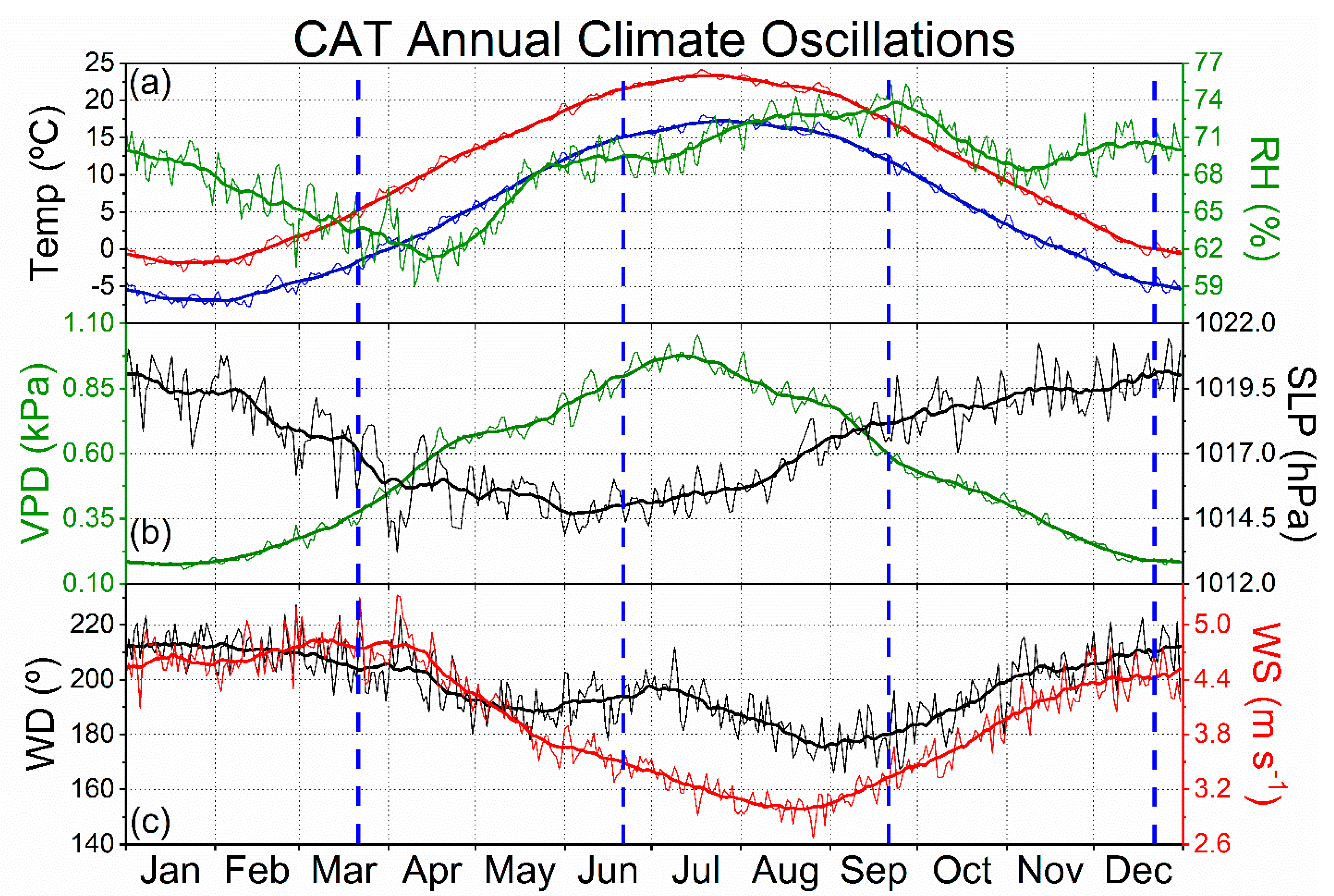
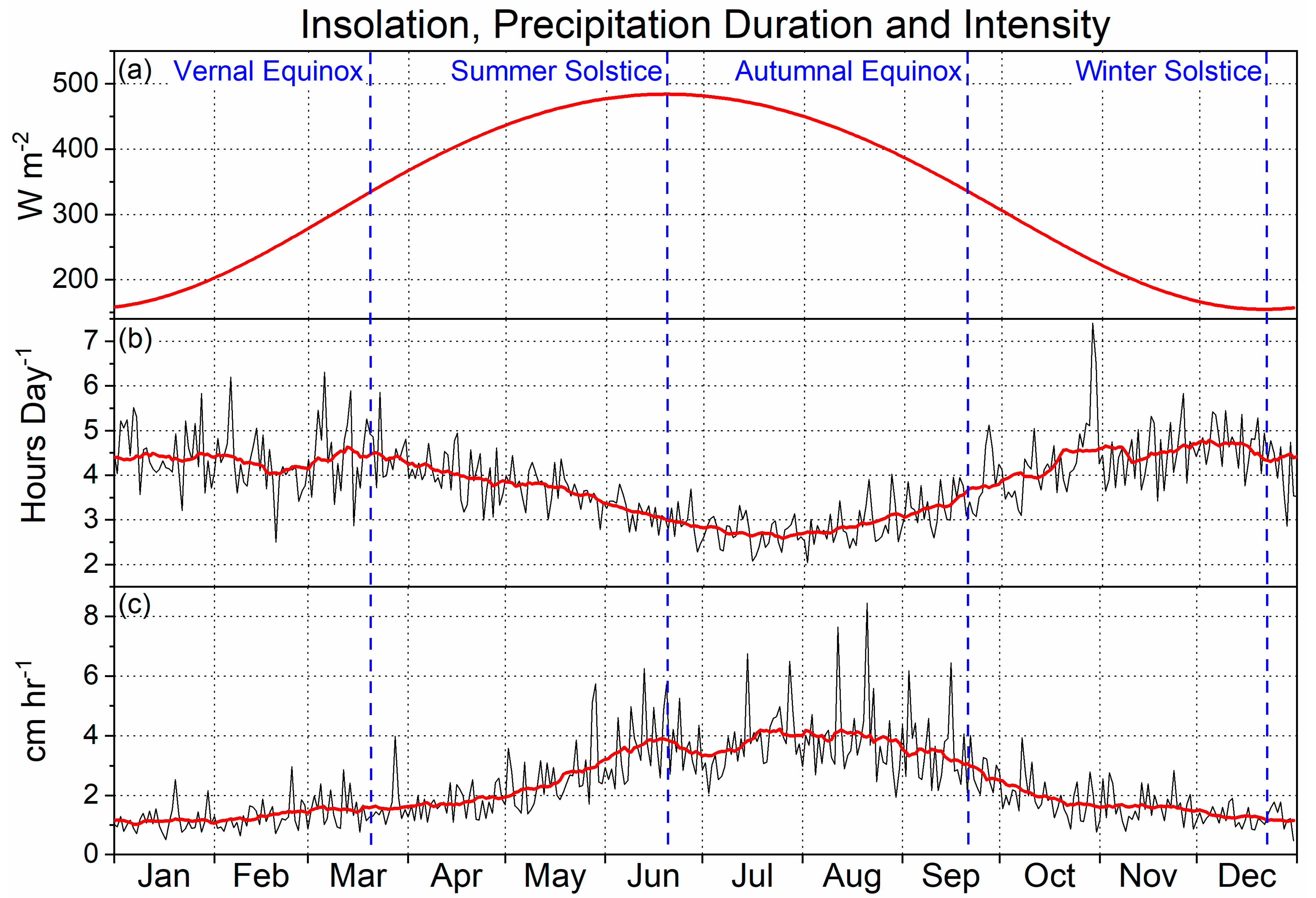
3.1. Annual CAT Climate

The annual oscillations of ambient temperature (Ta), dew point temperature (Td), relative humidity (RH) averaged along all CAT stations are presented in Figure 3a. The centered moving averages (CMAs) of Ta attained maximum and minimum values of 23.4 °C and −1.8 °C on 24 July and 26 January, respectively. The maximum and minimum Ta lagged summer (21 June) and winter (21 December) solstices by 34 and 37 days, respectively. Similarly, average Td increased from a minimum of −6.9 °C on 4 February to a maximum of 17.3 °C on 25 July indicating the maximum and minimum values lagged for each solstice by 35 and 46 days, respectively. The average VPD values increased from a minimum of 0.17 kPa on 16 January to a maximum of 0.98 kPa on 11 July (Figure 3b) indicating the minimum and maximum VPD values lagged insolation by 27 and 21 days, respectively. The annual oscillations of Ta, Td, and VPD were nearly synchronized, but the annual oscillation of RH was distinct. The maximum and minimum RH values of 73.9% and 61.2% occurred on 24 September and 15 April, respectively. As a result, the minimum and maximum RH values lagged winter and summer solstices by 96 and 116 days, respectively. The average SLPs decreased from a maximum of 1020.2 hPa on 26 December to a minimum of 1014.7 hPa of 3 July. As a result, the minimum and maximum SLP lagged winter and summer solstices by 195 and 189 days, respectively. The maximum and minimum wind speed (WS) values of 4.8 m·s−1 and 3.0 m·s-1 occurred on 12 March and 21 August and lagged summer and winter solstices by 265 and 244 days, respectively (Figure 3c). Similarly, the maximum and minimum wind direction (WD) values of 213.3° and 175.4° occurred on 2 February and 29 August and lagged summer and winter solstices by 227 and 252 days, respectively. Consequently, the annual oscillations of Ta, Td, and VPD lagged that of insolation by approximately one month, RH lagged insolation by approximately one season, SLP lagged insolation by approximately two seasons, and WS and WD lagged insolation by approximately three seasons.

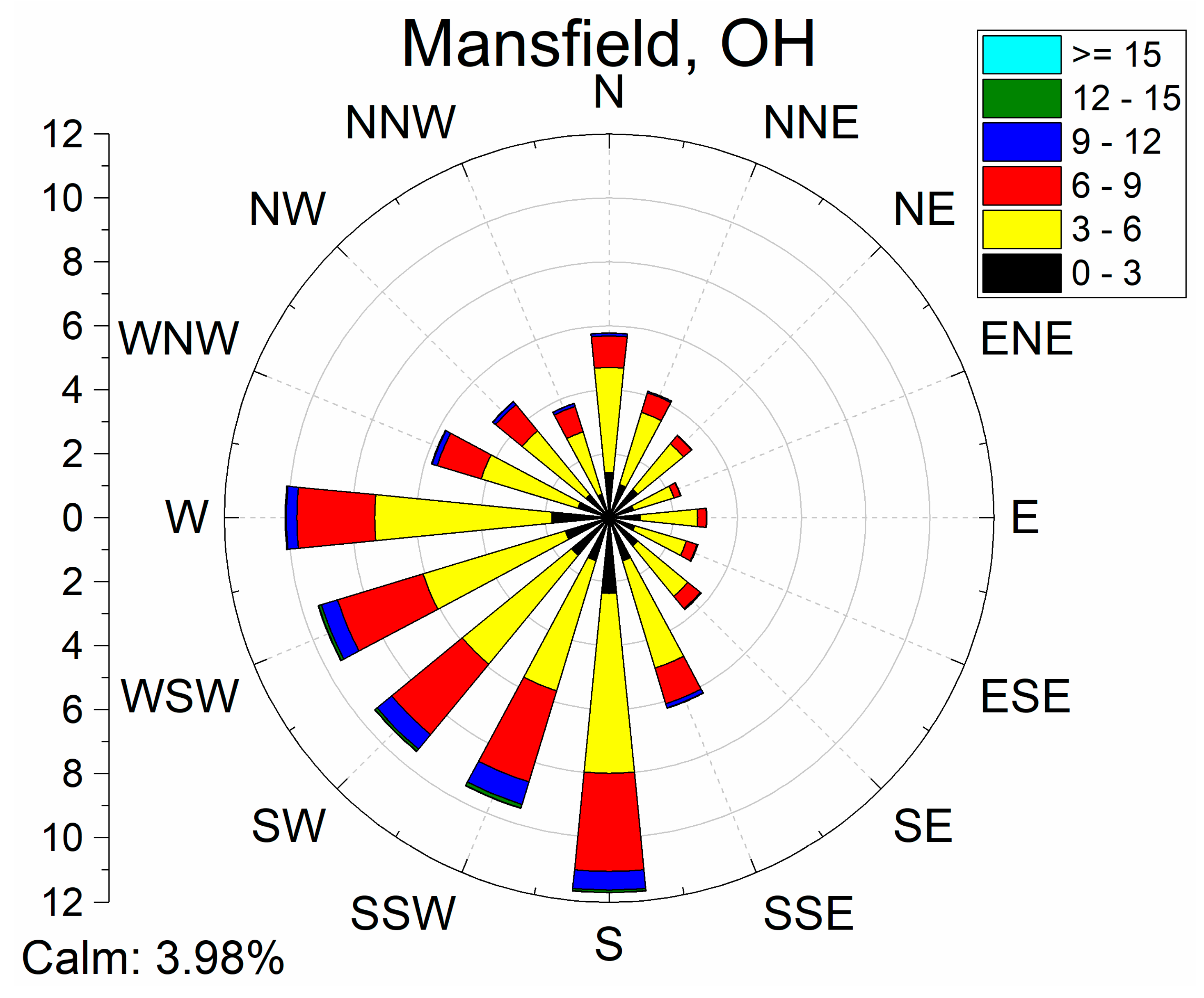
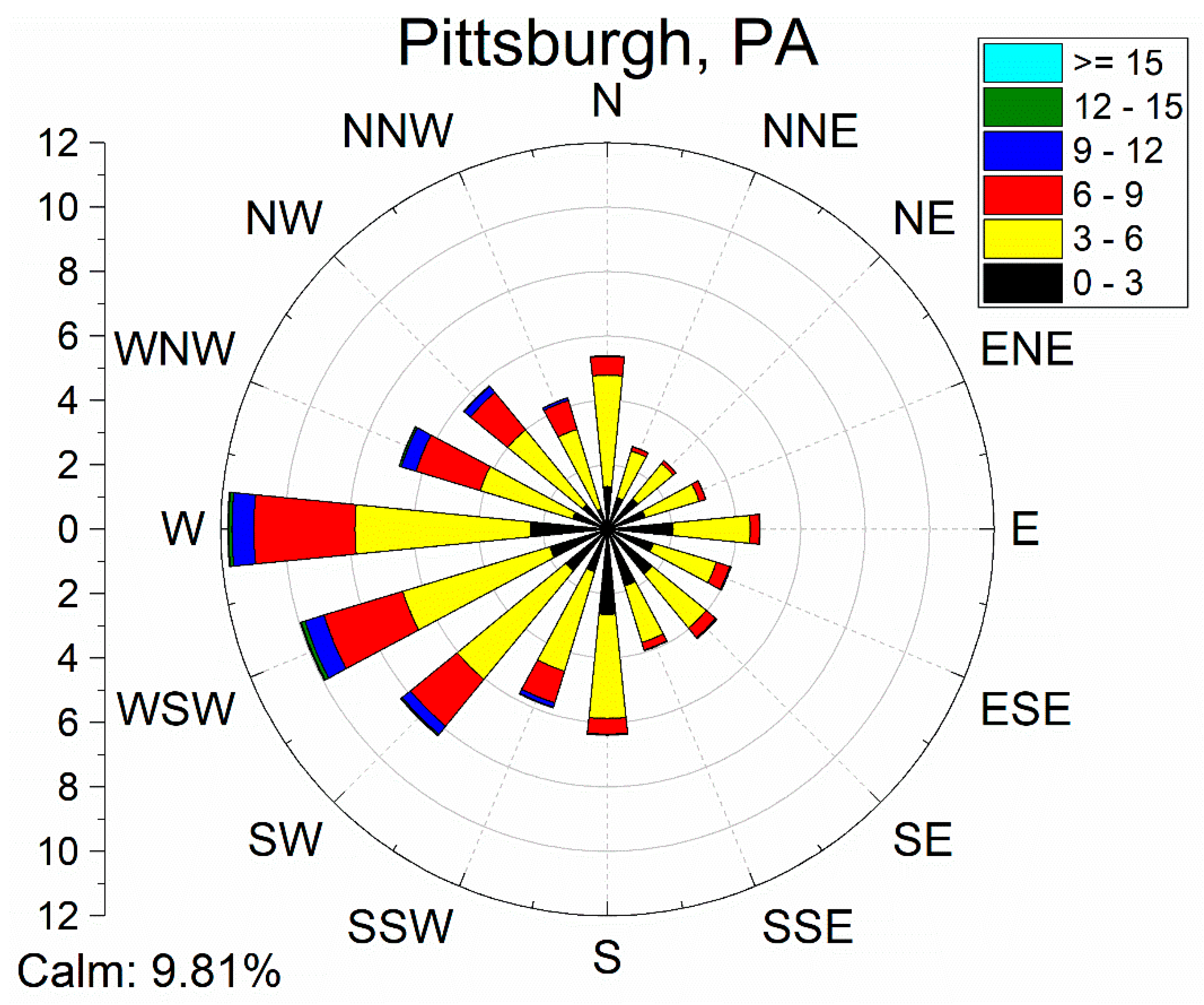
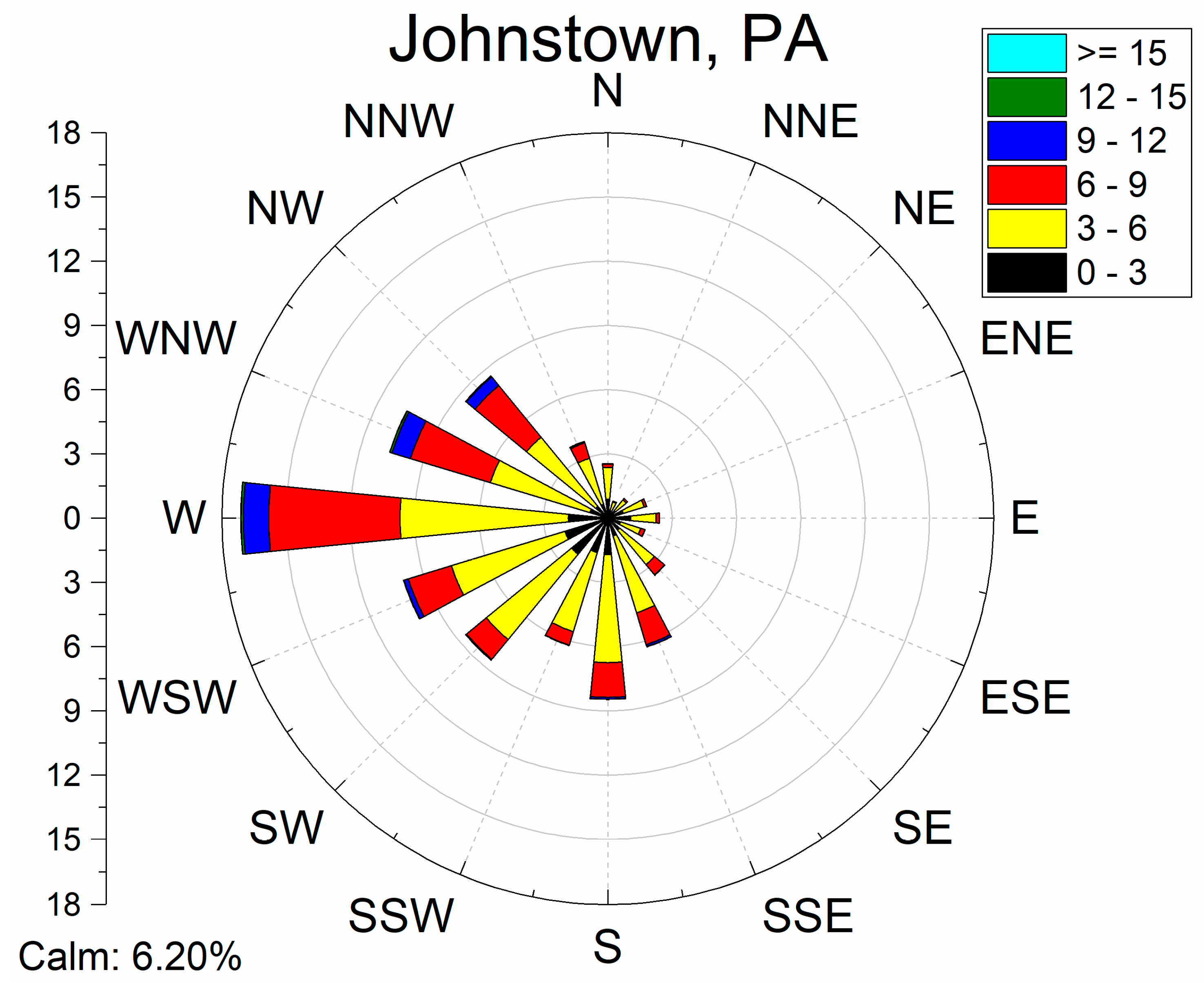
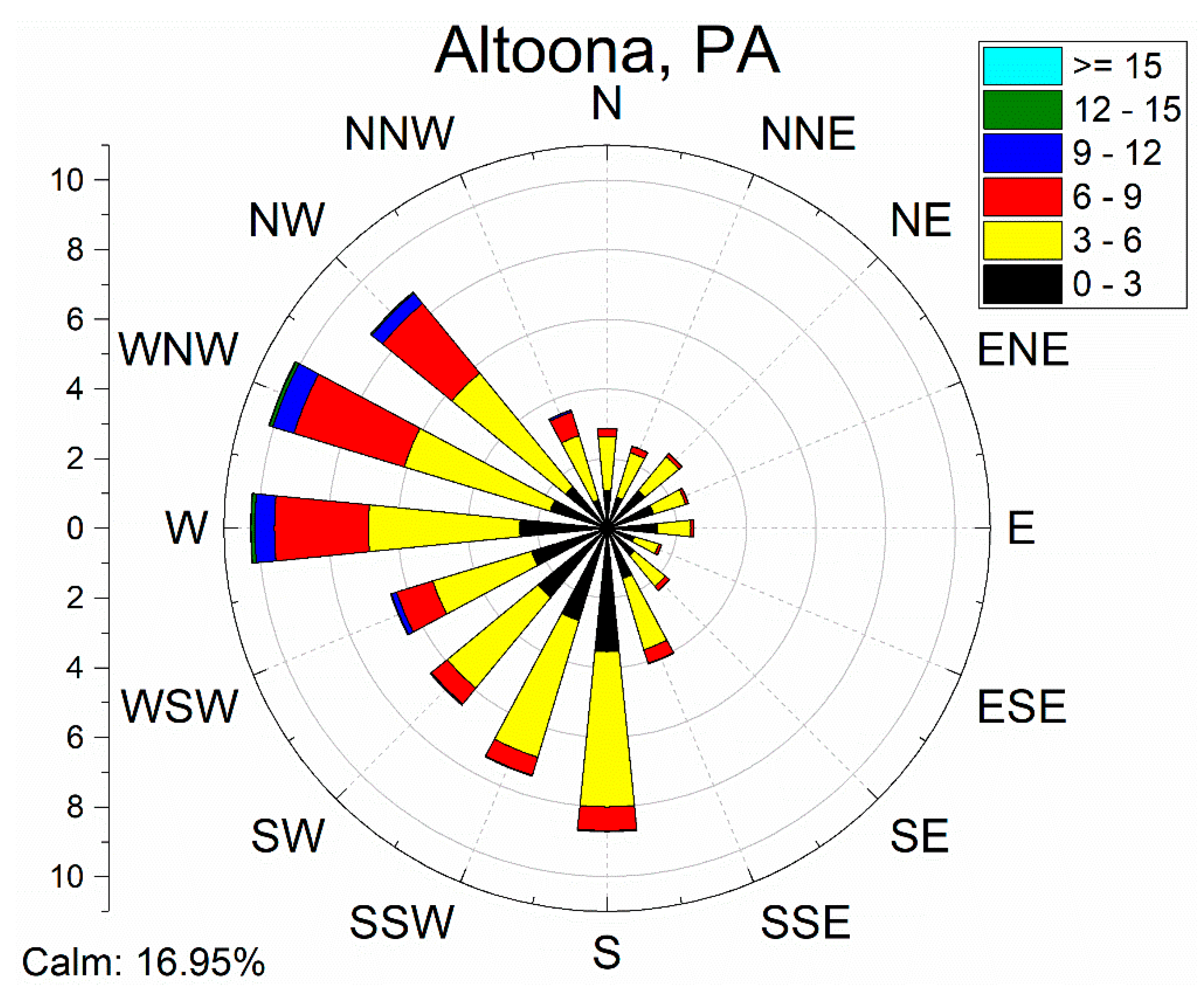
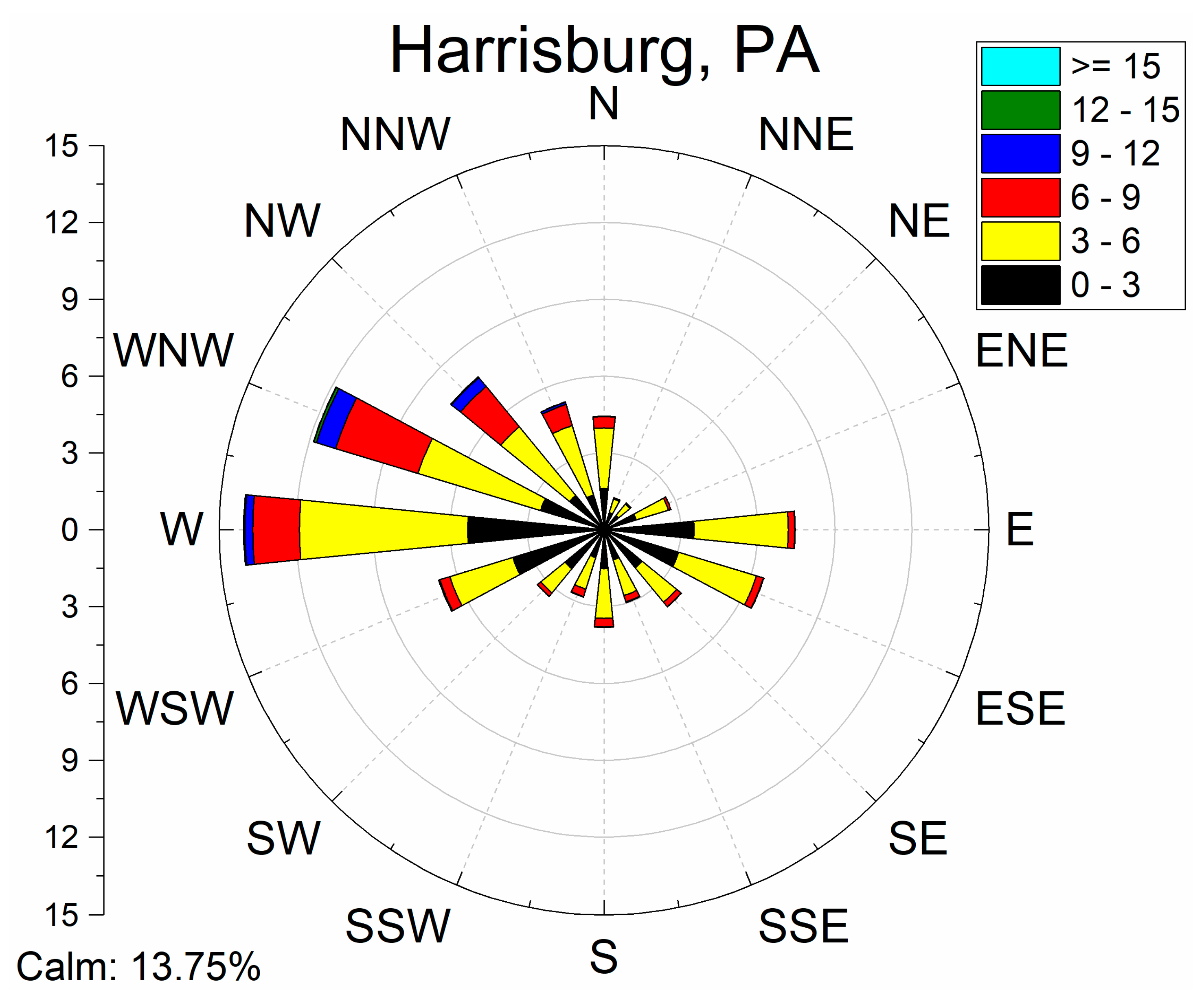
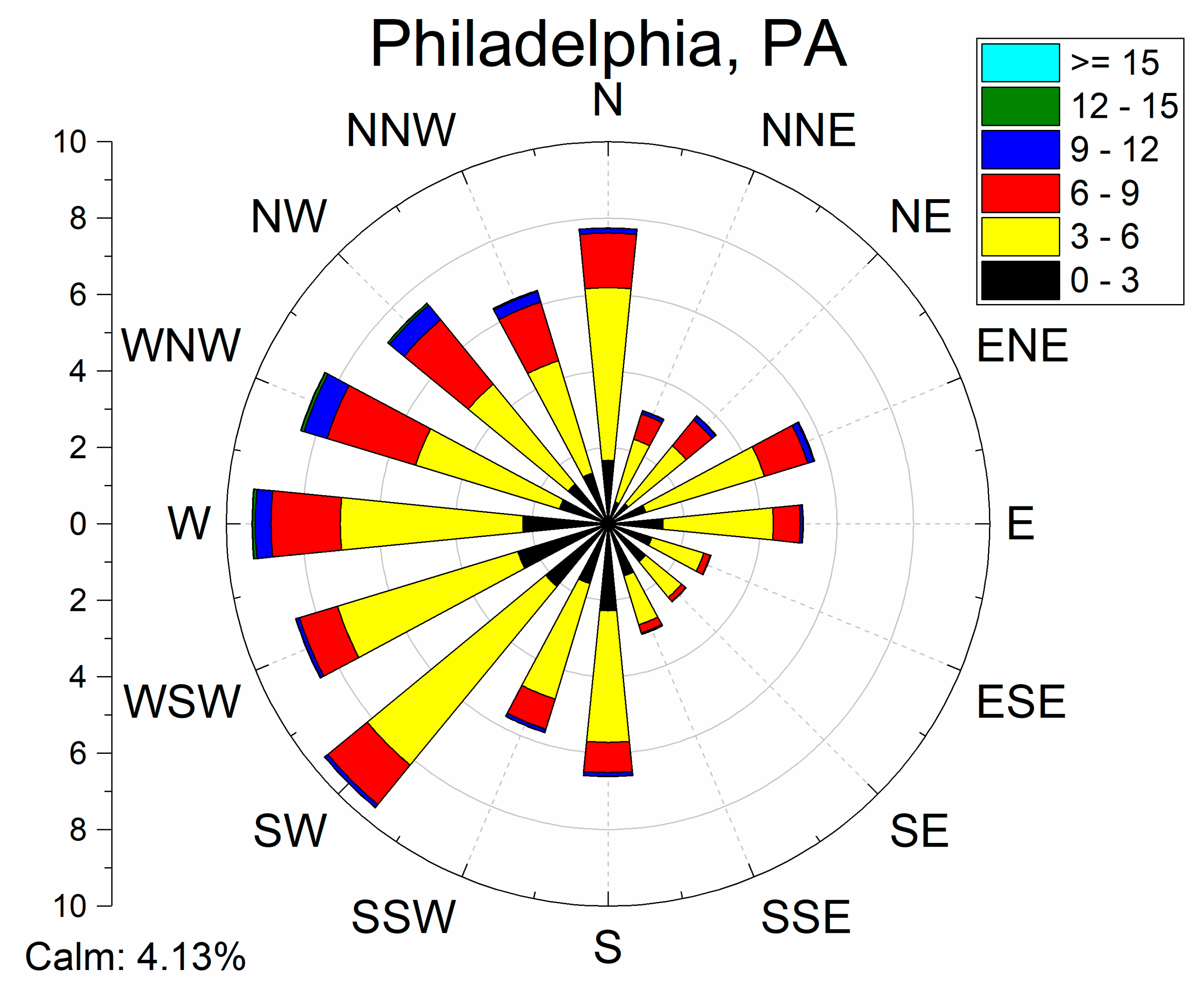
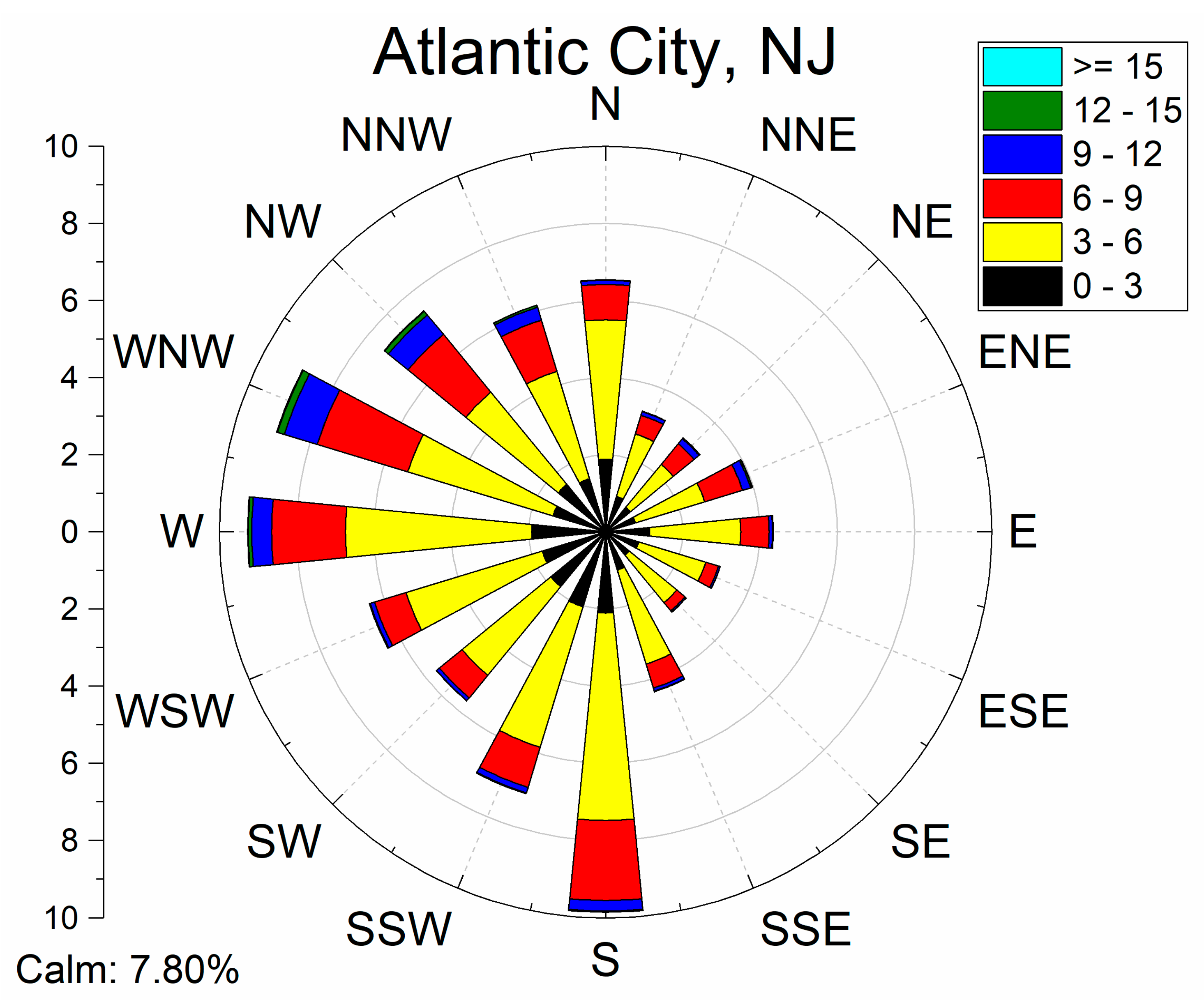
3.2. CAT Wind Direction

Raw wind observations at each airport were separated into 16 equal sized bins and results are summarized in Table 2 and traditional wind rose diagrams for each CAT site is available in the Appendix A (Figure A1, Figure A2, Figure A3, Figure A4, Figure A5, Figure A6 and Figure A7). Averaged along the CAT, north-northeasterly (NNE) winds were least common (2.5%) and westerly winds were most common (11.7%) and westerly winds were the most common WD bin at five of the CAT airports. WDs with some easterly component (i.e., NNE-SSE) accounted for a CAT average of 23.4% of WD observations. At individual airports, easterly, southerly, westerly, and northerly winds were most common at CXY (7.5%), MFD (11.7%), JST (17.1%), and PHL (7.8%), respectively. However, air currents flowing over or around local topographic features likely influenced WD distributions at each airport. For example, valley locations east of the Allegheny Front (AF) included AOO and CXY where calm winds were observed for 17.0% and 13.8% of each airport respective period of record. To put this in perspective, winds were calm at AOO for 71,201 h of the 420,066 h long period of record (Table 1). The highest elevation airport (JST; 696 m) was positioned on an exposed ridgeline (Figure 2) where westerly winds were observed 17.1% of the time. Similarly, MFD was positioned on the western margin of the Allegheny Plateau where southerly winds were most frequent and calm winds were least frequent. Despite prevailing westerly WDs, easterly winds represented an average of 23.4% of WD observations and substantial location-specific variability existed along the CAT.

3.3. Ambient CAT Environment

The descriptive statistics of each variable throughout the period of record (POR) were summarized for each station along the CAT in Table 3. On average, the highest elevation site (JST) had the coolest ambient (Ta; 9.2 °C) and dew point (Td; 3.8 °C) temperatures. Alternatively, the lowest elevation site (PHL) had the warmest average Ta (12.9 °C) and the site positioned on the Atlantic Ocean’s coast (ACY) had the warmest average Td (6.8 °C). Combined, longitudinal gradients in ambient and dew point temperatures were well-correlated with elevation (R = 0.97; 0.80) indicating average lapse rates of −5.25 °C·km−1 and -3.61 °C·km−1, respectively. The standard deviation and inter-quartile range (IQR) of Ta generally decreased from west (11 °C; 18.3 °C) to east (10 °C; 16.2 °C), but longitudinal differences in Td were more complex. Ta and Td distributions were characterized by negative skewness at all sites indicating Ta and Td values below the median were more common than a normal distribution. In particular, stations west of the AF (AF) had more negatively skewed Ta distributions (skewness ≤ −0.22) than sites to the east (skewness ≥ −0.16). All CAT sites were characterized by negative Ta and Td kurtosis indicating extreme Ta and Td values were uncommon relative to a normal distribution and the most negative kurtosis values were at stations east of the AF. In particular, maximum Ta and Td skewness (−0.09; −0.24) and minimum Ta and Td kurtosis (−0.86; −0.84) occurred at CXY. However, the AF separated sites characterized by minimum Ta and Td skewness (JST; ACY) and maximum Ta and Td kurtosis (ACY; MFD). MFD and CXY were the most and least humid sites (71.8%; 64.6%) with the smallest and largest IQRs (28.1%; 34.3%) and standard deviations (18.0%; 20.5%), respectively. JST had the smallest average (0.45 kPa) and standard deviation (0.48 kPa) of VPD values, but the three largest mean and median VPD values and the three smallest mean and median RH values occurred at PIT, CXY, and PHL. Relative to the highest elevation station (JST), the decrease in average RH at CXY (6.3%) was approximately double that observed at PIT (3.1%) consistent with elevation differences between JST and either CXY (590 m) or PIT (301 m; Table 1). Elevation explained most of the VPD variability along the CAT (R2 = 0.61) and with the exception of CXY and PHL, skewness and kurtosis of VPD values increased from west-to-east indicating VPD values above the median were most common and most extreme at ACY. As a result, the AMS in general and the AF in particular demarcates physiographic provinces with distinct statistical properties of fundamental atmospheric variables (i.e., air masses).

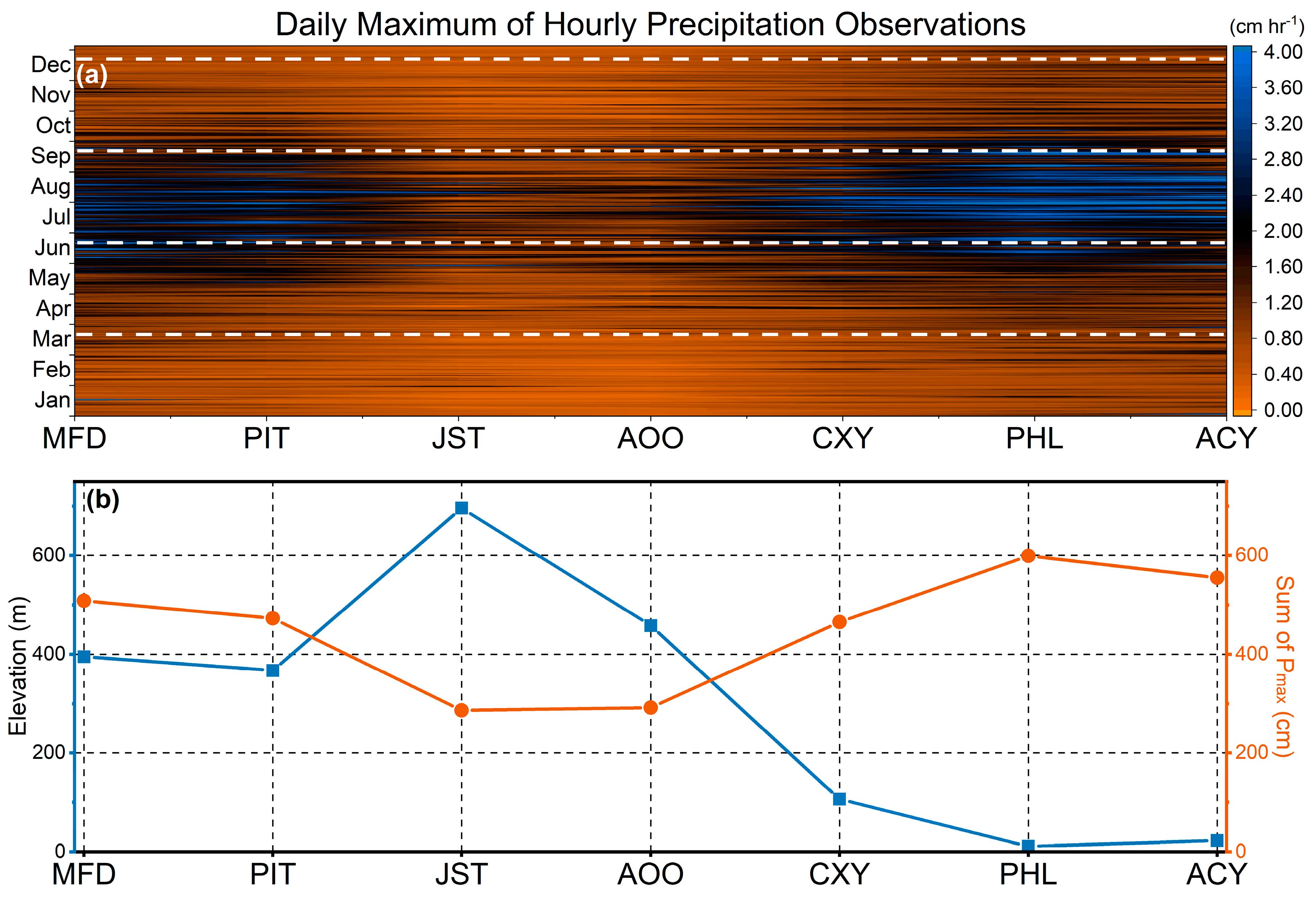
3.4. CAT Precipitation Regimes

Along the CAT, stratiform precipitation regimes may be characterized by long duration (>4 h) and low intensity (<2 cm·h−1) whereas convective precipitation regimes may be characterized by short duration (<4 h) and high intensity (>2 cm·h−1; Figure 4). Averaged along the CAT, maximum and minimum precipitation durations of 4.8 and 2.6 h occurred on 4 December and 25 July, respectively. Similarly, precipitation duration exceeded four hours per day between 14 October and 16 April along the CAT indicating midpoint dates of stratiform and convective precipitation regimes occurred on 13 January and 16 July, respectively (Figure 4b). As a result, the midpoint dates of long and short duration precipitation regimes lagged winter and summer solstices by 24 and 26 days, respectively. Temporally smoothed (i.e., CMA) maximum CAT precipitation rates rose from an absolute minimum of 1.0 cm·h−1 on 7 January to an absolute maximum of 4.23 cm·h−1 on 25 July. The smoothed maximum precipitation rates along the CAT were less than 2 cm·h−1 between 12 October and 2 May indicating midpoint dates for stratiform and convective precipitation regimes of 21 January and 22 July, respectively. Thus, the midpoint dates of both low and high intensity precipitation regimes lagged winter and summer solstices by 32 days.
The absolute maximum precipitation rate (8.46 cm·h−1; Figure 4) was recorded in Atlantic City, NJ on 21 August, 1997 when a series of thunderstorms resulted in a storm total rainfall of 34.29 cm (Table 3; [49]). Similarly, extreme precipitation rates (> 6 cm·h−1) occurred at MFD on 13 June, 2017 (6.25 cm·h−1), ACY on 15 July, 2015 (6.76 cm·h−1), CXY on 12 August, 2010 (7.65 cm·h−1), and PHL on 3 September, 2000 (6.17 cm·h−1), 7/28/2013 (6.50 cm·h−1), and 16 September,2017 (6.45 cm·h−1). The maximum precipitation rates observed at PIT (5.44 cm·h−1), JST (5.11 cm·h−1), and AOO (4.60 cm·h−1) occurred on 28 July, 1999, 28 May, 2012, and 9 September, 2004, respectively. Despite short PORs at AOO and JST, the maximum precipitation rates at the other five locations occurred during the final 18 years of their respective POR suggesting maximum precipitation rates are comparable. The longitudinal gradient in maximum precipitation rates along the CAT indicates maxima at all CAT sites were well constrained by astronomical season dates (Figure 5a). Additionally, the sum of daily precipitation rate maxima (Figure 5b) indicates an absolute maximum at PHL (599 cm) where the IQR and standard deviation of precipitation rates was at maximum (Table 4). The ratio of daily precipitation rate maxima to station elevation (not shown) was well constrained west of the AF (0.41 < ratio < 1.29) relative to ratios east of the AF (0.64 < ratio < 54.48). On the Allegheny Plateau (MFD; PIT), within the AMS (JST; AOO), and east of the AMS (CXY, PHL, ACY) average ratios were 1.29, 0.52, and 27.67, respectively. As a result, large precipitation rates were least common at high elevations where standard deviation was minimized and most common east of the AMS where standard deviations were maximized (Table 4).

4. Discussion

4.1. Annual Climate Oscillations

Analyzing climate statistics in relation to geologic features and astronomic dates is valuable because both are physically relevant to the Earth’s climate system and stable on time scales associated with anthropogenic climate change [50]. The annual oscillation of CAT average Ta lagged that of insolation by 35.5 days. This is because radiant energy exchange occurs at the soil or vegetation surface and turbulent eddies transport accumulated heat to the height of standard METAR observation (1.5 m; [35,46]). The vapor pressure deficit (VPD) and atmospheric moisture content (Td) lagged insolation by an average of 24 and 40.5 days, respectively. The temporal patterns of Td and VPD are similar to that of Ta because soils and vegetated surfaces represent diurnally modulated sources (evaporation) and sinks (condensation) of water vapor [46,51]. However, at longer time scales (e.g., monthly), synoptic scale advection of latent and sensible heat represents a similarly important modulator of Ta, Td, and VPD [52]. The North Atlantic Subtropical High (i.e., Bermuda High) is a semi-permanent synoptic scale feature that enhances poleward advection of subtropical moisture plumes, especially on its western periphery during the warm season [53,54]. The Gulf of Mexico and Atlantic Ocean represent source regions for subtropical moisture plumes that often result in heavy rainfall along the CAT, especially east of the Allegheny Front (AF) where exposure and trajectories are more favorable [28]. The seasonality of air mass source regions may be identified by the annual oscillation of RH that lagged insolation by an average of 106 days. As a result, spring and fall equinoxes approximate the maximum frequency of arid continental and moist subtropical air masses along the CAT, respectively. Thus, the annual oscillations of fundamental atmospheric variables lagged insolation by 24 to 106 days due to convection (i.e., high Reynolds number) and advection (i.e., low Reynolds number) occurring over a spectrum of spatiotemporal scales.
Atmospheric flow (i.e., wind speed [WS] and direction [WD]) is induced by a force balance involving gradients in sea level pressure (SLP), the Coriolis force, centrifugal acceleration, and friction [55]. SLP gradients represent the most variable force and synoptic scale pressure perturbations (i.e., extratropical cyclones [ETC] and anticyclones) induce strong winds that are most common during the winter months, but cold, dry, and dense (i.e., large SLP) continental air masses prevailed along the CAT (Figure 3; [4]). Mesoscale pressure perturbations (e.g., gravity waves; differential heating) are omnipresent and often contribute to the initiation of thunderstorms in the presence of buoyant warm season air masses [9]. As a result, the summertime SLP minimum is particularly important because differential heating of the CAT’s complex terrain focuses thunderstorm development along ridgelines that often propagates to adjacent slopes [9,56]. Furthermore, the moist atmospheric currents funneled into steep AMS valleys can focus repeated redevelopment of terrain-locked thunderstorms that can result in flash flooding and debris flows associated with precipitation rates exceeding 100 mm·h−1 for up to six hours [26,27,57]. In summary, a spatiotemporal spectrum of SLP perturbations modulate source regions of atmospheric currents and complex terrain can focus precipitation development, intensity, and flooding impacts.

4.2. CAT Winds

Despite knowledge of intricacies inherent to complex physiographic regions, prevailing winds and the resultant rain-shadow effect are most commonly cited [4,9,10]. Indeed, winds with a westerly component represented between 50.9% (PHL) and 64.9% (JST) of WD observations at each CAT airport (CAT average of 54.5%) indicating the majority of weather events were embedded within prevailing westerly winds. In particular, the climatological distribution of precipitation is often modulated by WD (i.e., rain-shadow), but the influence of WD on precipitation regimes and cloud water deposition is not well understood [28,58,59]. West of the AF, the largest rainfall rates have been associated with well-organized and rapidly-moving thunderstorm complexes embedded within the warm sector of ETCs that are more commonly referred to as mesoscale convective systems (MCSs; [27,60]). Most notably, an MCS on 18 July, 1942 resulted in a world record rainfall accumulation of 780 mm in 4.75 h at Smethport, PA (166 km north of JST; [25]). Some MCSs can maintain intensity while traversing the AMS while others dissipate upon encountering the AMS’s rugged terrain posing a problem for heavy rainfall forecasting [61]. Alternatively, cloud water deposition (CWD) is a substantial albeit gradual hydrologic input, especially for high-elevation forests in eastern North America [58]. CWD is a function of cloud moisture content, droplet size distribution and velocity, and characteristics of the landscape intersecting cloud moisture. Notably, CWD is not a function of wind direction indicating that a substantial fraction of CWD’s hydrologic input within the AMS may occur within easterly air currents originating from the Atlantic Ocean. Therefore, further investigation of weather within non-prevailing WDs is needed, especially related to distinguishing precipitation regimes that may contribute to the region’s changing bioclimatic diversity [62,63].
Winds with an easterly component represented between 17.9% (JST) and 26.0% (PHL) of WD observations at each CAT airport (CAT average of 23.4%) indicating prevailing winds misrepresented many weather events along the CAT. Between 1949 and 2003, four catastrophic flash flooding events east of the AF were embedded within easterly subtropical moisture currents being funneled into east-facing river valleys [27]. In these rare situations, east facing river valleys can focus repeated thunderstorm development resulting in locally catastrophic flash flooding in locations often described as a rain-shadow. Alternatively, severe winter weather hazards including ice accretion and heavy snowfall east of the AF are associated with cold-air damming (CAD) events [2]. CAD occurs when the kinetic energy of buoyant air currents is inadequate to displace relatively dense air masses entrenched along east-facing slopes (i.e., Froude number; [2]). Additionally, CAD influences the trajectory and intensification of ETCs year-round [64], but impacts are often greatest within the Ridge and Valley province where entrenched winter air masses can result in ecologically impactful ice storms [65,66]. Thus, warm and cool season weather extremes resulting in substantial socioeconomic (e.g., flood damage; [27]) and biological (e.g., reduced canopy cover; [65]) implications are linked to easterly flow regimes within the AMS. Therefore, weather events embedded within air currents traversing the AMS—from all directions—need to be investigated further in the context of the AMS’s socioeconomic well-being and bioclimatic diversity.
Wind speed (WS) influences the bulk aerodynamic conductance of terrestrial ecosystems [67] indicating calm winds influence bioclimatic diversity by modulating exchanges of energy, mass, and momentum that are fundamental to ecosystem form and function [46]. Averaged along the CAT, calm winds represented 9% of all hourly observations and low elevation valleys within the Ridge and Valley Province (AOO [17%]; CXY [13.8%]) that were characterized by the greatest proportion of calm winds. Considering WS observations at METAR sites were positioned 10m above the ground [37], calm winds indicate a stagnant surface layer at least 10 m thick where turbulent fluxes of heat, mass, and momentum approach zero [46]. Stagnant surface layers limit terrestrial ecosystem fluxes and are favorable for fog formation that commonly results in hazardous travel conditions within the AMS region [68,69]. The AMS’s spectrum of ridge and valley dimensions (Figure 2) may be related to spatiotemporal characteristics of turbulent fluxes that are more challenging to quantify. PIT observed calm winds 9.8% of the time exemplifying the spatial spectrum of ridges and valleys, because PIT was positioned on a local ridge (367m) within a mesoscale (~300 km) valley between MFD (395 m) and JST (696 m; Table 1; Figure 2). Thus, WD and WS modulate turbulent fluxes across a broad range of spatiotemporal scales. This suggests that quantitative analysis of the region’s roughness will improve understanding of bioclimatic diversity in the AMS and other mountainous regions globally.
Irrespective of WD or WS, adiabatic compression and warming of air currents descending the AMS results in environmental lapse rates approaching the dry adiabatic lapse rate (9.8 °C·km−1) that is a common lower-tropospheric feature on days when tornadoes are observed [70]. For example, springtime ETCs east of the Rocky Mountains often result in westerly mid-tropospheric air currents characterized by steep mid-level lapse rates intersecting southerly lower-tropospheric air currents transporting rich Gulf of Mexico moisture [71]. The frontal boundaries at the intersection of converging air masses often initiate springtime thunderstorms that when combined with steep lapse rates and directional wind shear, result in supercell thunderstorms [71]. Due to their ability to produce tornadoes, large hail, severe wind gusts, and flash flooding, supercells are one of the most destructive weather phenomena in the United States [72]. The region where supercells occur most frequently is commonly referred to as tornado alley, but tornadoes are observed in every U.S. state suggesting less focused analysis is justified [73,74]. Despite tornado observations throughout the AMS [75] and an observed eastward shift in United States tornado frequency [76], relatively little is known about the mechanistic influence of the AMS on regional tornadogenesis [77]. A local maximum in tornado observation frequency existed across the Piedmont and Coastal Plain provinces where ACY’s moister climate intersects air currents descending the AMS. Importantly, an agglomeration of urban development is focused within this region including PHL’s metropolitan population of more than 6 million residents [16,40,74] suggesting an increasing risk of severe thunderstorm hazards including flooding and tornadoes by the end of the 21st century [78]. It is therefore of great concern that tornadogenesis in proximity to the AMS is becoming more frequent considering dense urban development, limited regional understanding, and greater focus on canonical regions farther west.

4.3. Long-term CAT Climate

Descriptive and higher order statistics indicated that atmospheric currents flowing over and around CAT topography, especially the Allegheny Front (AF), resulted in distinct probability distributions of Ta, Td, RH, and VPD (Table 3). The standard deviation and inter-quartile range (IQR) of Ta generally decreased from west (11 °C; 18.3 °C) to east (10 °C; 16.2 °C) consistent with a gradient between variable continental and temperate maritime temperature regimes [79]. However, Ta and Td skewness and kurtosis was negative at all CAT airports indicating values below the median were more common and extreme values were less common across the AMS region than a normal distribution implies, respectively [33]. In particular, average Ta skewness and kurtosis at airports west of the AF (−0.24; −0.77) were 78.6% smaller and 4.2% larger than airports east of the AF (−0.13; −0.80), respectively. Substantially more skewed Ta distributions west of the AF may emphasize the climatic importance of prevailing westerly winds ascending versus descending the AF [9]. However, observations and MFD and PIT, located west of the AF, indicated 25.6% and 25.7% of WD observations had an easterly component, respectively. This suggests that air currents traversing the AMS result in a bidirectional rain-shadow. For example, PIT’s mean and median values of Ta, Td, and VPD were 4.9% and 5.4% warmer, 10.7% and 6.1% cooler, and 23.1% and 10.2% larger than MFD, respectively which was consistent with easterly air currents descending the AF (Table 3). However, MFD was positioned 62 km away from the coastline of Lake Erie (25,667 km2; [80]) and 222m above Lake Erie’s mean water level (173 m ASL; [80]). This implies that an adiabatic expansion and cooling of the Great Lakes’ humid maritime climate could influence regional bioclimatic diversity. Thus, the Great Lakes may counteract effects of a bidirectional rain-shadow considering the largest average RH (71.8%) and smallest median VPD (0.26 kPa) occurred at MFD (Table 3).
In the context of a bidirectional AMS rain-shadow, moisture removed by precipitation and interception processes embedded within air currents traversing the AMS may explain differences in higher order statistics along the CAT. The maximum skewness and minimum kurtosis of Td distributions occurred east of the AF, but the decreasing distance to the Atlantic Ocean had the opposite effect consistent with maritime climates (Table 3; [79]). As a result, low elevation valleys within the broader Ridge and Valley province experienced extreme Ta and Td values most often (i.e., large kurtosis), but observations near the median were more common than other CAT airports (i.e., small skewness). Farther west, AMS peaks and ridges (e.g., JST) were characterized by the smallest average Ta, Td, and VPD values and the most negatively skewed Ta distribution indicative of a more severe high elevation climate [4]. On the deeply dissected Allegheny Plateau, valleys spanning a spectrum of spatial scales were skewed toward cooler and more humid conditions (Table 3) consistent with the influence of North America’s Great Lakes (244,160 km2 [80]). In nearby West Virginia, USA long term trends (1900-2016) in maximum and minimum Ta converged and year-to-year variance decreased [30]. The decreasing temperature variability suggests skewness and kurtosis of Ta and Td becomes more negative across the AMS region that may exacerbate ongoing forest species composition changes (oak to maple) of North America’s Eastern Deciduous Forest [63]. The skewness and kurtosis of Ta and Td observations suggested that AMS’s physiographic provinces were characterized by distinct bioclimatic regimes [81,82,83] that justified increased observation density within the AMS’s region and other similarly complex regions globally.
VPD values represent the concentration gradient between saturated and ambient air and are particularly relevant to physiological processes that often distinguish bioclimatic zones, because the evaporating surface of organisms (e.g., stomata) often approaches saturation [46]. JST had the smallest average (0.45 kPa) and standard deviation (0.48 kPa) of VPD values. This implies that the relatively common cloud immersion along AMS ridgelines (Table 3) contributes between 14% and 31% of plant available water [84]. In addition to supplying water, cloud immersion influences photosynthetic light quality and quantity while reducing water vapor exchange rates [22]. Furthermore, cloud water is often characterized by ionic concentrations up to an order of magnitude greater than rain water indicating a substantial contribution to total chemical deposition [58]. The median VPD values at PIT, CXY, and PHL were 18.5%, 40.8%, and 48.2% larger than that of JST, respectively. This indicates that substantially greater atmospheric evaporative demand may increase precipitation recycling when soils are moist [85] or induce drought during dry periods. The physical constraints of RH (0% ≤ RH ≤ 100%) and VPD (≥ 0 kPa) values influenced skewness and kurtosis of each variable [33], but comparisons between sites may be useful. For example, VPD skewness and kurtosis were 15.3% and 38.8% smaller at MFD than at ACY suggesting advection of air masses modified by North America’s Great Lakes (244,160 km2 [80]) and the AMS within northwesterly flow regimes, respectively (Table 2 and Table 3). More broadly, airports west of the AF were characterized by average VPD skewness and kurtosis values of 7.9% and 22.1% smaller than airports east of the AF. Furthermore, the median VPD values were 14.3% larger east of the AF. This indicates that low elevation valleys east of the AF (e.g., CXY and PHL) may be more susceptible to drought. However, site-specific drought vulnerability assessments in the AMS region should include the local slope, the aspect, and species compositions [86]. Alternatively, substantially drier ambient conditions characterized by steep low level lapse rates may increase the frequency of hazardous convective weather for locations, such as Ellicott City, MD, USA [87]. Ultimately, the often cited rain-shadow phenomena [8,9] may insufficiently describe differences in mesoscale precipitation regimes within the AMS and other regions characterized by complex terrain, globally [10].

4.4. CAT Precipitation Regimes

Precipitation regimes along the CAT were modulated by insolation (Figure 4a) indicating extremes of stratiform and convective precipitation regimes were seasonally constrained by a relatively constant aspect of the Earth’s climate system [88]. The midpoint dates of both stratiform and convective precipitation intensities lagged insolation by 32 days indicating time scales more similar to ocean-atmosphere feedbacks (1–2 months; [89]) than that of land-atmosphere feedbacks (~10 days; [90]). The temporal lag of approximately a month suggests timing of each precipitation regime corresponds with seasonality of moisture advection from oceanic sources such as the Bermuda High that is maximized during boreal summer [53,54]. The midpoint dates of long and short duration precipitation regimes lagged insolation by six to eight days more than midpoints of precipitation intensity suggesting the CAT’s diurnal maximum of convective intensity [91] lagged insolation more than global scale baroclinic instability [92]. However, a local maximum in average maximum intensity of 3.91 cm·hr−1 (June 19th) coincided with the summer solstice (Figure 4c). This suggests a more nuanced lead-lag relationship between insolation and convective precipitation regimes at intra-annual time scales (e.g., soil moisture-precipitation coupling; [93]) that should be investigated further.
On average, the combination of cool temperatures and small insolation during the cool season (November through April) often results in elevated soil moisture concentrations. As a result, up to 40% of annual flood peaks at long-term (>75 year POR) USGS gauging stations near the CAT occurred during March and April were associated with extratropical cyclone passage, snowmelt, and rain on snow events [27]. The interactions between frontal boundaries and mountain barriers have been particularly relevant to spring flooding, because up to 80% of the initially linear cold fronts were slowed and deformed by the AMS [64]. On average, cold front slowed by 40% prolonging precipitation and representing a potential mechanism for more frequent North American weather extremes, including flooding [94,95,96]. Alternatively, the combination of large insolation, convective precipitation regimes, and warm temperatures integrated throughout the warm season (May through October) results in the regions’ climatological minimum in antecedent soil [27]. Despite reduced summertime soil moisture, the extreme convective precipitation rates can exceed soil infiltration rates on AMS slopes (16 to 117 mm·h−1; [97]) resulting in flash flooding, especially in smaller catchments (e.g., Rapidan River; [26]). The Allegheny Plateau observed half as many annual flood peaks during October or November as the Ridge and Valley province [27] suggesting physiographic provinces were characterized by distinct flooding regimes. Thus, additional investigation is needed to better understand the variable influence of observed [30] and projected [98] increases in precipitation on each physiographic province.
Despite a period of record dating back to 1948, the five most extreme precipitation rates (>6.17 cm·hr-1) were observed between 2010 and 2017. This suggests that super Clausius-Clapeyron scaling [29] of convective precipitation regimes could be particularly relevant to the AMS region. Smaller maximum precipitation rates at AOO and JST (<5.11 cm·hr-1; Table 2) indicate high elevation ridges and inter-mountain valleys may be less susceptible to extreme convective precipitation events than adjacent lower elevation slopes [9]. However, Johnstown, PA experienced severe flooding from a rain-on-snow event on 17 March, 1936 and a nocturnal MCS on 19-20 July,, 1977, suggesting the entire AMS region was vulnerable to stratiform and convective flooding threats [99]. Despite vulnerabilities, the higher saturation vapor pressures at lower elevations enhance microphysical droplet growth processes [9,100] and thunderstorm outflow often triggers renewed convective updrafts on adjacent slopes [101,102,103]. Furthermore, moist atmospheric currents originating from the Atlantic Ocean can result in heavy rainfall on slopes with southeasterly aspects whereas inter-mountain valleys and the adjacent Allegheny plateau (e.g., PIT, JST, and AOO) are sheltered from Atlantic moisture [28]. In summary, extreme precipitation rates along the CAT were most frequent east of the AF during July, August, and September and recent events suggest hourly precipitation rates have increased since 1948.

4.5. Summary and Future Work

The Appalachian Mountain System (AMS) represents one of North America’s most ecologically diverse regions resulting from extensive physiographic complexity and climatic heterogeneity contained between the Mississippi River basin, the Great Lakes region, and the Atlantic Ocean. The current work advances understanding of hydroclimatic heterogeneity of the AMS region using hourly observations of a suite of meteorological variables collected over a long period of record (1948–2017). The traditional rain-shadow explanations of precipitation patterns assumed prevailing wind patterns that were insufficient within the AMS where 45.5% of weather events were embedded within non-prevailing wind currents. Flash flooding associated with orographic thunderstorms or wintry weather associated with cold air damming were both associated with easterly air currents. The annual sums of maximum precipitation rates occurred east of the AMS. This implies that a geographically induced convective maximum near PHL needs to be investigated further. In particular, whether or not the boundary between Piedmont and Coastal Plains provinces (i.e., Fall Line [41]) is sufficiently prominent to focus convective development needs to be determined. Furthermore, fog-water deposited on AMS vegetation associated with moist wind currents ascending ridges from any direction or, to a lesser extent, the lack of wind within sheltered valleys is a common occurrence within the AMS. Fog and dew water are underappreciated water inputs that should be observed more extensively to improve understanding of ecological diversity and better manage increasingly strained water resources. The Allegheny Front is a particularly prominent ridgeline that represents a physical bi-directional barrier to horizontal moisture advection that may be important for delineating water mass exchange regimes within the AMS and many other locations globally. Equinoxes and solstices are physically relevant to climate across a range a spatial scale but are static on time scales of recent climatic changes indicating further investigation of climatic changes relative to astronomical dates is warranted. The current work established annual oscillations of fundamental atmospheric variables lagged insolation by 24 to 106 days along the CAT due to convection and advection occurring across a spectrum of spatiotemporal scales that should be observed more extensively. Ultimately, a great deal of future work is needed to better understand relations between weather, biologic diversity (e.g., forest species composition), and local to regional vulnerabilities (e.g., flooding) of the broader AMS region and many other locations globally.

5. Conclusions

The analysis of hourly meteorological observations indicated spatial and temporal heterogeneity of fundamental atmospheric variables that were independent of elevation. The long-term averages of ambient temperature were well correlated with airport elevation (R2 = 0.97), but elevation explained less dew point temperature (R2 = 0.80) and vapor pressure deficit (R2 = 0.61) heterogeneity. The adiabatic modulation of air currents traversing the AMS likely contributed to maximum standard deviation of Td and VPD observed at CXY, whereas minimum values were observed at JST. The combination of adiabatic processes and proximity to the Great Lakes and Atlantic Ocean variably influenced skewness and kurtosis of Ta, Td, and VPD. The minimum Ta skewness occurred at JST, whereas minimum Td skewness occurred at ACY indicating observations below median Ta and Td values were most common at high elevations and near the Atlantic Ocean, respectively. Similarly, skewness and kurtosis of VPD indicated values above the median were most common and farthest from the median near warm Atlantic Ocean waters (ACY), whereas cool Great Lakes waters had the opposite effect at MFD. The large water bodies supply atmospheric water vapor to stratiform and convective precipitation regimes that were shown to lag winter and summer solstices by 24 and 32 days, respectively. Precipitating storms are often assumed to be embedded within prevailing wind currents (i.e., rain-shadow) that represents just 54.5% of wind direction observations indicating the AMS represents a barrier to omnidirectional moisture advection. The sum of daily maximum precipitation rates indicated a local maximum at PHL (599 cm) where precipitation rates exceeded 6 cm·h−1 three times since 3 August, 2000. Ultimately, the current work draws attention to substantial mesoscale climatic variability inherent to complex physiography whose links to changing water resources and ecological diversity should be investigated further to better prepare communities for climatic vulnerabilities (e.g., flooding).

Author Contributions

Conceptualization, J.H. and E.K.; methodology, E.K. and J.H.; formal analysis, E.K.; investigation, E.K.; data curation, E.K.; writing—original draft preparation, E.K.; writing—review and editing, J.H.; visualization, E.K. and J.H.; supervision, J.H.; project administration, J.H.; funding acquisition, J.H.

Funding

This work was supported by the National Science Foundation under Award Number OIA-1458952, the USDA National Institute of Food and Agriculture, Hatch project 1011536, and the West Virginia Agricultural and Forestry Experiment Station. Results presented may not reflect the views of the sponsors and no official endorsement should be inferred.

Acknowledgments

In this section you can acknowledge any support given which is not covered by the author contribution or funding sections. This may include administrative and technical support, or donations in kind (e.g., materials used for experiments).

Conflicts of Interest

The authors declare no conflicts of interest. The funders had no role in the design of the study; in the collection, analyses, or interpretation of data; in the writing of the manuscript, or in the decision to publish the results.

Appendix A

Figure A1. Wind rose diagram for Mansfield (MFD), Ohio, USA. Wind speeds are presented in m·s−1 and winds were split into 16 directional bins.
Climate 07 00091 g0a1
Figure A2. Wind rose diagram for Pittsburgh (PIT), Pennsylvania, USA. Wind speeds are presented in m·s-1 and wind direction was split into 16 directional bins.
Climate 07 00091 g0a2
Figure A3. Wind rose diagram for Johnstown (JST), Pennsylvania, USA. Wind speeds are presented in m·s−1 and wind direction was split into 16 directional bins.
Climate 07 00091 g0a3
Figure A4. Wind rose diagram for Altoona (AOO), Pennsylvania, USA. Wind speeds are presented in m·s−1 and wind direction was split into 16 directional bins.
Climate 07 00091 g0a4
Figure A5. Wind rose diagram for Harrisburg (CXY), Pennsylvania, USA. Wind speeds are presented in m·s−1 and wind direction was split into 16 directional bins.
Climate 07 00091 g0a5
Figure A6. Wind rose diagram for Philadelphia (PHL), Pennsylvania, USA. Wind speeds are presented in m·s−1 and wind direction was split into 16 directional bins.
Climate 07 00091 g0a6
Figure A7. Wind rose diagram for Atlantic City (ACY), New Jersey, USA. Wind speeds are presented in m·s−1 and wind direction was split into 16 directional bins.
Climate 07 00091 g0a7

References

  1. Smith, R.B. The Influence of Mountains on the Atmosphere. Earth 1979, 21, 87–230. [Google Scholar]
  2. Bell, G.D.; Bosart, L.F. Appalachian cold-air damming. Mon. Weather Rev. 1988, 116, 137–161. [Google Scholar] [CrossRef]
  3. Warren, R.J., II. An experimental test of well-described vegetation patterns across slope aspects using woodland herb transplants and manipulated abiotic drivers. New Phytol. 2010, 185, 1038–1049. [Google Scholar] [CrossRef] [PubMed]
  4. Barry, R.G. Mountain Weather and Climate, 3rd ed.; Cambridge University Press: Cambridge, UK, 2008; ISBN 9780511754753. [Google Scholar]
  5. Müller, H. On the radiation budget in the alps. J. Climatol. 1985, 5, 445–462. [Google Scholar] [CrossRef]
  6. Katata, G. Fogwater deposition modeling for terrestrial ecosystems: A review of developments and measurements. J. Geophys. Res. 2014, 119, 8137–8159. [Google Scholar] [CrossRef]
  7. Greenland, D. Spatial distribution of radiation in the Colorado Front Range. Climatol. Bull. 1978, 24, 1–14. [Google Scholar]
  8. Barry, R.G.; Chorley, R.J. Atmosphere, Weather and Climate; Routledge: Abingdon, UK, 2009. [Google Scholar]
  9. Houze, R.A., Jr. Orographic effects on precipitating clouds. Rev. Geophys. 2012, 50, 1–47. [Google Scholar] [CrossRef]
  10. Stockham, A.J.; Schultz, D.M.; Fairman, J.A.A.G.; Draude, A.A.P. Quantifying the rain-shadow effect: Results from the peak district, british isles. Bull. Am. Meteorol. Soc. 2018, 99, 777–790. [Google Scholar] [CrossRef]
  11. United States Department of Agriculture, F.S. Monongahela National Forest Land and Resource Management Plan. Available online: https://www.fs.usda.gov/Internet/FSE_DOCUMENTS/stelprdb5330420.pdf (accessed on 15 February 2018).
  12. Rodgers, J. Tectonics of the Appalachians; Wiler-Interscience: New York, NY, USA, 1970. [Google Scholar]
  13. Richardson, A.D.; Lee, X.; Friedland, A.J. Microclimatology of treeline spruce-fir forests in mountains of the northeastern United States. Agric. For. Meteorol. 2004, 125, 53–66. [Google Scholar] [CrossRef]
  14. Dickson, R.R. Some Climate-Altitude Relationships in the Southern Appalachian Mountain Region. Bull. Am. Meteorol. Soc. 1959, 40, 352–359. [Google Scholar] [CrossRef]
  15. Mittelbach, G.G.; Mittelbach, G.G.; Schemske, D.W.; Schemske, D.W.; Cornell, H.V.; Cornell, H.V.; Allen, A.P.; Allen, A.P.; Brown, J.M.; Brown, J.M.; et al. Evolution and the latitudinal diversity gradient: speciation, extinction and biogeography. Ecol. Lett. 2007, 10, 315–331. [Google Scholar] [CrossRef] [PubMed]
  16. Raitz, K.B.; Ulack, R. Appalachia A Regional Geography Land, People, and Development; Westview Press, Inc.: Boulder, CO, USA, 1984. [Google Scholar]
  17. Cogbill, A.C.V.; White, P.S. The Latitude-Elevation Relationship for Spruce-Fir Forest and Treeline along the Appalachian Mountain Chain along the Appalachian relationship for spruce-fir mountain chain forest and treeline. Vegetatio 2013, 94, 153–175. [Google Scholar] [CrossRef]
  18. Smathers, G.A. Fog interception on four southern Appalachian mountain sites. J. Elisha Mitchell Sci. Soc. 1982, 98, 119–129. [Google Scholar]
  19. Baumgardner, R.E.; Isil, S.S.; Lavery, T.F.; Rogers, C.M.; Mohnen, V.A. Estimates of cloud water deposition at mountain acid deposition program sites in the appalachian mountains. J. Air Waste Manag. Assoc. 2003, 53, 291–308. [Google Scholar] [CrossRef] [PubMed]
  20. Johnson, D.M.; Smith, W.K. Low clouds and cloud immersion enhance photosynthesis in understory species of a southern Appalachian spruce-fir forest (USA). Am. J. Bot. 2006, 93, 1625–1632. [Google Scholar] [CrossRef]
  21. Richardson, A.D.; Denny, E.G.; Siccama, T.G.; Lee, X. Evidence for a rising cloud ceiling in eastern North America. J. Clim. 2003, 16, 2093–2098. [Google Scholar] [CrossRef]
  22. Johnson, D.M.; Smith, W.K. Cloud immersion alters microclimate, photosynthesis and water relations in Rhododendron catawbiense and Abies fraseri seedlings in the southern Appalachian Mountains, USA. Tree Physiol. 2008, 28, 385–392. [Google Scholar] [CrossRef]
  23. Kunkel, K.E.; Easterling, D.R.; Kristovich, D.A.R.; Gleason, B.; Stoecker, L.; Smith, R. Meteorological Causes of the Secular Variations in Observed Extreme Precipitation Events for the Conterminous United States. J. Hydrometeorol. 2012, 13, 1131–1141. [Google Scholar] [CrossRef]
  24. Colle, B.A.; Booth, J.F.; Chang, E.K.M. A Review of Historical and Future Changes of Extratropical Cyclones and Associated Impacts Along the US East Coast. Curr. Clim. Chang. Rep. 2015, 1, 125–143. [Google Scholar] [CrossRef] [Green Version]
  25. Eisenlohr, W.S. Floods of July 18, 1942 in north-central Pennsylvania. In U.S. Geological Survey Water Supply Papers; U.S. G.P.O.: Washington, DC, USA, 1951; pp. 59–158. [Google Scholar]
  26. Smith, J.A.; Baeck, M.L.; Steiner, M.; Miller, J. Catastrophic rainfall from an upslope thunderstorm in the central Appalachians: The Rapidan storm rainfall accumulations exceeding a 6-h period during the morning and afternoon of Virginia flooding extending from. Water Resour. Res. 1996, 32, 3099–3113. [Google Scholar] [CrossRef]
  27. Villarini, G.; Steiner, M.; Smith, J.A.; Ntelekos, A.A.; Baeck, M.L. Extreme rainfall and flooding from orographic thunderstorms in the central Appalachians. Water Resour. Res. 2011, 47, 1–24. [Google Scholar]
  28. Konrad II, C.E. Moisture Trajectories Associated With Heavy Rainfall in the Appalachian Region of the United States. Phys. Geogr. 1994, 15, 227–248. [Google Scholar] [CrossRef]
  29. Lenderink, G.; Barbero, R.; Loriaux, J.M.; Fowler, H.J. Super-Clausius-Clapeyron scaling of extreme hourly convective precipitation and its relation to large-scale atmospheric conditions. J. Clim. 2017, 30, 6037–6052. [Google Scholar] [CrossRef]
  30. Kutta, E.; Hubbart, J.A. Changing climatic averages and variance: Implications for mesophication at the eastern edge of North America’s Eastern deciduous forest. Forests 2018, 9. [Google Scholar] [CrossRef]
  31. Crozier, M.J. Deciphering the effect of climate change on landslide activity: A review. Geomorphology 2010, 124, 260–267. [Google Scholar] [CrossRef]
  32. Bishop, D.A.; Pederson, N. Regional Variation of Transient Precipitation and Rainless-day Frequency Across a Subcontinental Hydroclimate Gradient. J. Extrem. Events 2015, 2. [Google Scholar] [CrossRef]
  33. Wilks, D.S. Statistical Methods in the Atmospheric Sciences, 3rd ed.; Academic Press: New York, NY, USA, 2011; ISBN 9780444515544. [Google Scholar]
  34. DeCarlo L T On the meaning and use of kurtosis. Psychol. Methods 1997, 2, 292–307. [CrossRef]
  35. Surface Weather Observations and Reports. Federal Meteorological Handbook; National Oceanic and Atmospheric Administration: Washington, DC, USA, 1988; 104p. [Google Scholar]
  36. Nadolski, V. Automated Surface Observing System User’s Guide. NOAA Publ. 1992, 12, 94. [Google Scholar]
  37. Nadolski, V.L. Automated Surface Observing System (ASOS) User’s Guide. Natl. Ocean. Atmos. Adm. Dep. Def. Fed. Aviat. Adm. United States Navy 1998, 74. [Google Scholar]
  38. National Oceanic and Atmospheric Administration Federal Standard for Siting Meteorlogical Sensors at Airports. U.S. Dep. Commer. 1994.
  39. Fujita, T.T. Tornadoes and downbursts in the context of generalized planetary scales. J. Atmos. Sci. 1981, 38, 1511–1534. [Google Scholar] [CrossRef]
  40. Annual Estimates of the Resident Population: April 1, 2010 to July 1, 2018; United States Census Bureau: Washington, DC, USA, 2019. Available online: https://factfinder.census.gov/faces/tableservices/jsf/pages/productview.xhtml?src=bkmk (accessed on 25 June 2019).
  41. Thwaites, F.T. Physiography of Eastern United States. Nevin M. Fenneman, 1st ed.; McGraw-Hill Book Company, Inc.: New York, NY, USA, 2009; Volume 47. [Google Scholar]
  42. Bothwell, M.P. Incline Planes and People—Some Past and Present Ones. West. Pennsylvania Hist. 1963, 46, 311–346. [Google Scholar]
  43. Lawther, D.E. Mount Washington: A Demographic Study of the Influence of Changing Technology. West. Pennsylvania Hist. 1981, 64, 44–72. [Google Scholar]
  44. Renner, G.T. The Physiographic Interpretation of the Fall Line. Geogr. Rev. 1927, 17, 278–286. [Google Scholar] [CrossRef]
  45. Buck, A.L. New Equations for Computing Vapor Pressure and Enhancement Factor. J. Appl. Meteorol. 1981, 20, 1527–1532. [Google Scholar] [CrossRef] [Green Version]
  46. Campbell, G.; Norman, J. An Introduction to Environmental Biophysics, 2nd ed.; Springer Science + Business Media, Inc.: New York, NY, USA, 1998; ISBN 0-387-94937-2. [Google Scholar]
  47. Rose, B.E.J. CLIMLAB: a Python toolkit for interactive, process-oriented climate modeling. J. Open Source Softw. 2018. [Google Scholar]
  48. Pietruszka, K. GEOCONTEXT-Profiler. Center for Geographic Analysis. 2011. Available online: http://www.geocontext.org/publ/2010/04/profiler/en/ (accessed on 15 March 2018).
  49. Smothers, R. Fast-Moving Storms Flood Slice of Southern New Jersey. New York Times. 1997. Available online: https://www.nytimes.com/1997/08/22/nyregion/fast-moving-storms-flood-slice-of-southern-new-jersey.html (accessed on 6 June 2018).
  50. Peixoto, J.P.; Oort, A.H. Physics of Climate; Spring: New York, NY, USA, 1992; ISBN 978-0-88318-712-8. [Google Scholar]
  51. Evett, S.; Prueger, J.H.; Tolk, J.A. Water and Energy Balances in the Soil-Plant-Atmosphere Continuum; CRC Press: Boca Raton, FL, USA, 2012; ISBN 978-1-4398-0305-9. [Google Scholar]
  52. Pierrehumbert, R.T. Evidence for Control of Atlantic by Large Scale Advection. Geophys. Res. Lett. 1998, 25, 4537–4540. [Google Scholar] [CrossRef]
  53. Li, W.; Li, L.; Fu, R.; Deng, Y. Changes to the North Atlantic Subtropical High and Its Role in the Intensification of Summer Rainfall Variability in the Southeastern United States. Bull. Am. 2010. [Google Scholar]
  54. Diem, J.E. Influences of the Bermuda High and atmospheric moistening on changes in summer rainfall in the Atlanta, Georgia region, USA. Int. J. Climatol. 2012, 33, 160–172. [Google Scholar] [CrossRef]
  55. Carlson, T.N. Mid-Latitude Weather Systems; Harper Collins Academic: Boston, MA, USA, 1991; ISBN 1-878220-30-6. [Google Scholar]
  56. Banta, R.M. The role of the mountain flow making clouds. Atmos. Process. Over Complex Terrain 1990, 23, 183–203. [Google Scholar]
  57. Kochel, R.C. Humid Fans of the Appalachian Mountains. In Alluvial Fans: A Field Approach; Rachocki, A.H., Church, M., Eds.; John Wiley and Sons Ltd.: New York, NY, USA, 1990; pp. 109–129. [Google Scholar]
  58. Vong, R.J.; Sigmon, J.T.; Mueller, S.F. Cloud Water Deposition to Appalachian Forests. Environ. Sci. Technol. 1991, 25, 1014–1021. [Google Scholar] [CrossRef]
  59. Lovett, G.M.; Kinsman, J.D. Atmospheric pollutant deposition to high-elevation ecosystems. Atmos. Environ. Part A Gen. Top. 1990, 24, 2767–2786. [Google Scholar] [CrossRef]
  60. Houze, R.a., Jr. Mesoscale Convective Systems-Review paper. Rev. Geophys. 2004, 42, 1–43. [Google Scholar] [CrossRef]
  61. Letkewicz, C.E.; Parker, M.D. Forecasting the Maintenance of Mesoscale Convective Systems Crossing the Appalachian Mountains. Weather Forecast. 2010, 25, 1179–1195. [Google Scholar] [CrossRef]
  62. Goetsch, C.; Wigg, J.; Royo, A.A.; Ristau, T.; Carson, W.P. Chronic over browsing and biodiversity collapse in a forest understory in Pennsylvania: Results from a 60 year-old deer exclusion plot. J. Torrey Bot. Soc. 2011, 138, 220–224. [Google Scholar] [CrossRef]
  63. Mcewan, R.W.; Dyer, J.M.; Pederson, N. Multiple interacting ecosystem drivers: toward an encompassing hypothesis of oak forest dynamics across eastern North America. Ecography (Cop.) 2011, 34, 244–256. [Google Scholar] [CrossRef]
  64. O’Handley, C.; Bosart, L.F. The Impact of the Appalachian Mountains on Cyclonic Weather Systems. Part I: A Climatology. Mon. Weather Rev. 1996, 124, 1353–1373. [Google Scholar] [CrossRef] [Green Version]
  65. Lafon, C.W. Forest disturbance by ice storms in Quercus forests of the southern Appalachian Mountains, USA. Ecoscience 2007, 13, 30–43. [Google Scholar] [CrossRef]
  66. Forbes, G.S.; Thomson, D.W.; Anthes, R.A. Synoptic and Mesoscale Aspects of an Appalachian Ice Storm Associated with Cold-Air Damming. Mon. Weather Rev. 1987, 115, 564–591. [Google Scholar] [CrossRef] [Green Version]
  67. Juang, J.-Y.; Stoy, P.; Novick, K.; Katul, G.; Siqueira, M. Separating the effects of albedo from eco-physiological changes on surface temperature along a successional chronosequence in the southeastern United States. Geophys. Res. Lett. 2007, 34. [Google Scholar] [CrossRef] [Green Version]
  68. Court, A.; Gerston, R.D. Fog Frequency in the United States. Geogr. Rev. 1966, 56, 543–550. [Google Scholar] [CrossRef]
  69. Mueller, A.S.; Trick, L.M. Driving in fog: The effects of driving experience and visibility on speed compensation and hazard avoidance. Accid. Anal. Prev. 2012, 48, 472–479. [Google Scholar] [CrossRef] [PubMed]
  70. Parker, M.D. Impacts of Lapse Rates on Low-Level Rotation in Idealized Storms. J. Atmos. Sci. 2011, 69, 538–559. [Google Scholar] [CrossRef]
  71. Doswell, C.A.; Carbin, G.W.; Brooks, H.E. The tornadoes of spring 2011 in the USA: An historical perspective. Weather 2012, 67, 88–94. [Google Scholar] [CrossRef]
  72. Folger, P. Severe Thunderstorms and Tornadoes in the United States; DIANE Publishing: Darby, PA, USA, 2013. [Google Scholar]
  73. Gagan, J.P.; Gerard, A.; Gordon, J. A historical and statistical comparison of “Tornado Alley” to “Dixie Alley”. Natl. Wea. Dig. 2010, 34, 145–155. [Google Scholar]
  74. Tippett, M.K.; Sobel, A.H.; Camargo, S.J. Association of U. S. tornado occurrence with monthly environmental parameters. Geophys. Res. Lett. 2012, 39, 2–7. [Google Scholar] [CrossRef]
  75. Gaffin, D.M.; Parker, S.S. A Climatology of Synoptic Conditions Associated with Significant Tornadoes across the. Weather Forecast. 2006, 21, 735–751. [Google Scholar] [CrossRef]
  76. Agee, E.; Larson, J.; Childs, S.; Marmo, A. Spatial redistribution of U.S. Tornado activity between 1954 and 2013. J. Appl. Meteorol. Climatol. 2016, 55, 1681–1697. [Google Scholar] [CrossRef]
  77. Bosart, L.F.; Seimon, A.; LaPenta, K.D.; Dickinson, M.J. Supercell Tornadogenesis over Complex Terrain: The Great Barrington, Massachusetts, Tornado on 29 May 1995. Weather Forecast. 2006, 21, 897–922. [Google Scholar] [CrossRef]
  78. Tippett, M.K.; Allen, J.T.; Gensini, V.A.; Brooks, H.E. Climate and Hazardous Convective Weather. Curr. Clim. Chang. Rep. 2015, 1, 60–73. [Google Scholar] [CrossRef] [Green Version]
  79. Rohli, R.V.; Vega, A.J. Climatology; Jones and Barttlett Publishers: Sudbury, MA, USA, 2008; ISBN 978-0-7637-3828-0. [Google Scholar]
  80. Fuller, K.; Shear, H.; Wittig, J. (Eds.) The Great Lakes. An Environmental Atlas and Resource Book, 3rd ed.; United States Environmental Protection Agency: Washington, DC, USA, 1995; ISBN 0-662-23441-3.
  81. Peet, R.K. Forest vegetation of the Colorado front range. Vegetatio 1981, 45, 3–75. [Google Scholar] [CrossRef]
  82. Goulden, M.L.; Anderson, R.G.; Bales, R.C.; Kelly, A.E.; Meadows, M.; Winston, G.C. Evapotranspiration along an elevation gradient in California’s Sierra Nevada. J. Geophys. Res. Biogeosciences 2012, 117, 1–13. [Google Scholar] [CrossRef]
  83. Morin, R.S.; Cook, G.W.; Barnett, C.J.; Butler, B.J.; Crocker, S.J.; Hatfield, M.A.; Kurtz, C.M.; Lister, T.W.; Luppold, W.G.; McWilliams, W.H.; et al. West Virginia Forests 2013. NRS-105. Newt. Square, PA US Dep. Agric. For. Serv. North. Res. Station. 2016, 128, 1–128. [Google Scholar]
  84. Berry, Z.C.; Hughes, N.M.; Smith, W.K. Cloud immersion: an important water source for spruce and fir saplings in the southern Appalachian Mountains. Oecologia 2014, 174, 319–326. [Google Scholar] [CrossRef] [PubMed]
  85. Dirmeyer, P.A.; Schlosser, A.C.; Brubaker, K.L. Precipitation, Recycling, and Land Memory: An Integrated Analysis. J. Hydrometeorol. 2009, 10, 278–288. [Google Scholar] [CrossRef]
  86. Fekedulegn, D.; Hicks, R.R.; Colbert, J.J. Influence of topographic aspect, precipitation and drought on radial growth of four major tree species in an Appalachian watershed. For. Ecol. Manage. 2003, 177, 409–425. [Google Scholar] [CrossRef]
  87. Thakali, R.; Bhandari, R.; Kandissounon, G.-A.A.; Kalra, A.; Ahmad, S. Flood risk assessment using the updated FEMA floodplain standard in the Ellicott City, Maryland, United States.; World Environmental and Water Resources Congress: Sacramento, CA, USA, 2017; pp. 280–291. [Google Scholar]
  88. Kopp, G.; Lean, J.L. A new, lower value of total solar irradiance: Evidence and climate significance. Geophys. Res. Lett. 2011, 38. [Google Scholar] [CrossRef] [Green Version]
  89. Gastineau, G.; Frankignoul, C. Influence of the North Atlantic SST variability on the atmospheric circulation during the twentieth century. J. Clim. 2015, 28, 1396–1416. [Google Scholar] [CrossRef]
  90. Ruiz-Barradas, A.; Nigam, S. Atmosphere – Land Surface Interactions over the Southern Great Plains: Characterization from Pentad Analysis of DOE ARM Field Observations and NARR. J. Clim. 2013, 26, 875–886. [Google Scholar] [CrossRef]
  91. Nesbitt, S.W.; Zipser, E.J. The Diurnal Cycle of Rainfall and Convective Intensity according to Three Years of TRMM Measurements. J. Clim. 2003, 16, 1456–1475. [Google Scholar] [CrossRef] [Green Version]
  92. Jablonowski, C.; Williamson, D.L. A baroclinic instability test case for atmospheric model dynamical cores. Q. J. R. Meteorol. Soc. 2006, 132, 2943–2975. [Google Scholar] [CrossRef] [Green Version]
  93. Wei, J.; Dirmeyer, P.A. Dissecting soil moisture-precipitation coupling. Geophys. Res. Lett. 2012, 39. [Google Scholar] [CrossRef]
  94. Francis, J.A.; Vavrus, S.J. Evidence linking Arctic amplification to extreme weather in mid-latitudes. Geophys. Res. Lett. 2012, 39. [Google Scholar] [CrossRef]
  95. Francis, J.A.; Vavrus, S.J. Evidence for a wavier jet stream in response to rapid Arctic warming. Environ. Res. Lett. 2015, 10, 014005. [Google Scholar] [CrossRef]
  96. Doswell, C.A.; Brooks, H.E.; Maddox, R.A. Flash Flood Forecasting: An Ingredients-Based Methodology. Weather Forecast. 1996, 11, 560–581. [Google Scholar] [CrossRef]
  97. Harden, C.P.; Scruggs, P.D. Infiltration on mountain slopes: a comparison of three environments. Geomorphology 2003, 55, 5–24. [Google Scholar] [CrossRef]
  98. Runkle, J.; Kunkel, K.E.; Frankson, R.; Stewart, B. West Virginia State Climate Summary; 2017; Available online: https://statesummaries.ncics.org/downloads/WV-print-2016.pdf (accessed on 6 June 2018).
  99. Lavine, M.P. The Johnstown Floods: Causes and Consequences. In Natural and Technological Disasters: Causes, Effects and Preventative Measures.; Majumdar, S.K., Forbes, G.S., Miller, E.W., Schmalz, R.F., Eds.; The Pennsylvania Academy of Science: Phillipsburg, NJ, USA, 1992; pp. 536–542. ISBN 978-0945809067. [Google Scholar]
  100. Frei, C.; Schär, C. A Precipitation Climatology of the Alps From High-Resolution Rain-Gauge Observations. Int. J. Climatol. 1998, 18, 873–900. [Google Scholar] [CrossRef]
  101. Mueller, C.K.; Carbone, R.E. Dynamics of a Thunderstorm Outflow. J. Atmos. Sci. 1986, 44, 1879–1898. [Google Scholar] [CrossRef]
  102. Moncrieff, M.W.; Liu, C. Convection Initiation by Density Currents: Role of Convergence, Shear, and Dynamical Organization. Mon. Weather Rev. 1999, 127, 2455–2464. [Google Scholar] [CrossRef]
  103. Moncrieff, M.W. The Multiscale Organization of Moist Convection and the Intersection of Weather and Climate. Geophys. Monogr. Ser. 2010, 189, 3–26. [Google Scholar]
Figure 1. Topographic map of the seven airports included in the cross Allegheny transect (Table 1) and urban and dense urban land uses. The map was created using ArcGIS® software by ESRI. ArcGIS® and ArcMap™ are the intellectual property of ESRI and are used herein under license. Copyright © ESRI.
Climate 07 00091 g001
Figure 2. The elevation profile of the cross Allegheny transect (CAT) with all seven airports selected for further investigation (Table 1).
Climate 07 00091 g002
Figure 3. Cross Allegheny Transect (CAT) daily average ambient temperature (red (a); °C), dew point temperature (blue (a); °C), and relative humidity (RH; green (a); %), CAT average vapor pressure deficit (VPD; green (b), kPa) and atmospheric pressure (AP; black (b); hPa), and CAT average wind direction (WD; black (c)) and speed (WS; red (c); m·s−1). The dashed vertical lines represent astronomical season dates.
Climate 07 00091 g003
Figure 4. Daily average incoming solar radiation at 40.2 °N ((a); W·m−2), Cross Allegheny Transect (CAT) average precipitation duration ((b); Hours Day−1), and maximum CAT precipitation rate (c; cm·h−1). Red lines on (b), (c) indicate three-week centered moving averages (CMAs). Dashed vertical blue lines represent astronomical season dates.
Climate 07 00091 g004
Figure 5. Daily maximum of hourly precipitation observations (cm·h−1) at each CAT location (a) and sum of daily precipitation rate maxima (Pmax [cm]; (b)) from west (MFD) to east (ACY) over each stations’ period of record (Table 1). Horizontal dashed lines in (a) represent astronomical season dates.
Climate 07 00091 g005
Table 1. The location, period of record (POR), and number of climatic observations for each selected airport along the cross Pennsylvania transect (CAT) in Pennsylvania, USA.
LatitudeLongitudeElevationP.O.R.Observations
Mansfield (MFD)40.82° N82.52° W395 m1948–2017 1437,882
Pittsburgh (PIT)40.49° N80.23° W367 m1949–2017571,954
Johnstown (JST)40.32° N78.83° W696 m1973–2017 *316,120
Altoona (AOO)40.30° N78.32° W458 m1949–2017 * 2420,066
Harrisburg (CXY)40.22° N76.85° W106 m1948–2017 3516,210
Philadelphia (PHL)39.87° N75.24° W11 m1948–2017608,283
Atlantic City (ACY)39.46° N74.58° W23m1948–2017555,004
* = No precipitation data until ASOS equipment was installed in 1999 (AOO) and 2000 (JST); 1 = Data gap (1 January 1955 to 10 November 1959); 2 = Data gaps (1 January 1955 to 31 December 1972) and (1 October 1976 to 30 June 1977); 3 = Data gap (15 May 1984 to 6 November 1984).
Table 2. The hourly wind direction (WD) observations separated into 16 directional bins throughout the period of record at each site along the Cross Allegheny Transect (CAT; Table 1). Light and dark gray shading represents minimum and maximum WD frequency for each CAT station, respectively. Underlined and italicized or bolded numbers represent minimum or maximum WD frequency for each WD, respectively.
Heading (°)MFDPITJSTAOOCXYPHLACYAvg CAT
Calm4.09.86.217.013.84.17.89.0
NNE22.54.12.70.82.51.33.13.32.5
NE453.42.81.22.81.43.73.22.6
ENE67.52.33.21.92.42.75.74.03.2
E903.04.72.42.57.55.14.34.2
ESE112.52.94.01.81.66.52.83.13.2
SE1353.74.43.52.33.92.62.73.3
SSE157.56.23.96.34.13.03.04.34.4
S18011.76.48.58.73.86.69.97.9
SSW202.59.55.86.27.42.85.77.16.4
SW2259.58.38.66.63.49.65.77.4
WSW247.59.510.010.06.56.78.66.48.2
W27010.111.817.110.214.19.39.311.7
WNW292.55.86.810.610.211.88.48.98.9
NW3154.75.88.68.87.77.57.47.2
NNW337.53.74.33.83.65.26.46.14.7
N3605.85.42.52.94.47.86.55.0
Avg = Average.
Table 3. Descriptive statistics of hourly ambient temperature (°C), dew point temperature (°C), relative humidity (%), vapor pressure deficit (kPa), and atmospheric pressure (kPa) observations throughout the period of record at each site along the Cross Allegheny Transect (CAT; Table 1). Bolded numbers represent maxima and underlined and italicized numbers represent minima.
CityMinMedMeanMaxIQRSt DevSkewKurt
Ambient Temp (°C)MFD−30.011.110.238.318.311.0−0.23−0.77
PIT−29.411.710.738.917.210.7−0.22−0.74
JST−27.710.09.236.717.410.6−0.26−0.80
AOO−31.210.610.238.917.110.3−0.16−0.79
CXY−26.212.212.040.617.310.4−0.09−0.86
PHL−21.713.312.940.016.710.2−0.12−0.85
ACY−23.312.812.439.416.210.0−0.16−0.71
Dew Point Temp (°C)MFD−37.15.64.927.216.110.2−0.28−0.70
PIT−35.05.04.626.816.610.1−0.29−0.76
JST−34.34.03.827.016.110.0−0.26−0.82
AOO−35.64.44.426.716.610.1−0.25−0.84
CXY−33.35.05.028.917.610.6−0.24−0.84
PHL−32.26.76.128.317.210.6−0.32−0.76
ACY−30.67.86.828.316.710.4−0.35−0.72
Relative Humidity (%)MFD4.173.771.8100.028.118.0−0.40−0.67
PIT4.769.567.8100.028.918.5−0.35−0.72
JST6.873.370.9100.029.218.6−0.47−0.59
AOO6.070.168.8100.028.818.7−0.30−0.71
CXY5.564.864.6100.034.320.5−0.13−0.99
PHL7.865.665.2100.033.720.1−0.14−1.00
ACY7.373.970.9100.033.220.0−0.45−0.81
VPD (kPa)MFD0.000.260.494.560.580.551.722.93
PIT0.000.320.545.420.590.571.753.07
JST0.000.270.454.830.530.481.753.41
AOO0.000.290.495.320.520.521.914.13
CXY0.000.380.625.920.640.631.853.86
PHL0.000.400.635.710.630.631.773.34
ACY0.000.300.515.370.540.562.034.79
St Dev = standard deviation, Skew = skewness, Kurt = kurtosis, Min = minimum, Med = median, Max = maximum, IQR = inter quartile range, Temp = Temperature, VPD = Vapor Pressure Deficit.
Table 4. Descriptive statistics of non-zero precipitation observations at each airport along the Cross Allegheny Transect (CAT; Table 1). Descriptive statistics of CAT maximum precipitation (cm·h−1) and daily average precipitation event duration (hours day−1). Bolded numbers represent maxima and underlined and italicized numbers represent minima.
nMinMedMeanMaxIQRSt DevSkewKurt
MFD347780.030.050.158.000.130.266.5982.22
PIT447640.030.050.135.440.100.226.4368.78
JST135380.030.050.135.110.130.226.6279.62
AOO116930.030.080.144.600.130.225.7856.46
CXY309820.030.080.157.650.150.246.4079.62
PHL426670.030.080.176.500.180.286.0360.79
ACY326780.030.080.188.460.180.286.8594.20
Maximum3660.461.942.318.461.751.311.282.02
Duration3662.043.853.857.411.240.860.370.23
N = sample size, Min = minimum, Med = median, Max = maximum, IQR = inter quartile range, St Dev = standard deviation, Skew = skewness, Kurt = kurtosis.

