Article

The Effect of Agulhas Eddies on Absorption and Transport of Anthropogenic Carbon in the South Atlantic Ocean

by
Iole B. M. Orselli
1,2,3,4,*,
Catherine Goyet
3,4,
Rodrigo Kerr
1,2,
José L. L. de Azevedo
1,
Moacyr Araujo
5,6,
Felippe Galdino
1,
Franck Touratier
3,4 and
Carlos A. E. Garcia
1,7
1
Laboratório de Estudos dos Oceanos e Clima, Instituto de Oceanografia, Universidade Federal do Rio Grande (FURG), Av. Itália km 8, s/n, Rio Grande, RS 96203-900, Brazil
2
Brazilian Ocean Acidification Network (BrOA), Av. Itália km 8, Rio Grande, RS 96203-900, Brazil
3
IMAGES_ESPACE-DEV, Université de Perpignan Via Domitia (UPVD), 52 ave. Paul Alduy, 66860 Perpignan, France
4
ESPACE-DEV UMR UG UA UM IRD, Maison de la télédétection, 500 rue Jean-François Breton, CEDEX 5, 34093 Montpellier, France
5
Laboratório de Oceanografia Física, Estuarina e Costeira (LOFEC), Departamento de Oceanografia, Centro de Tecnologia, Universidade Federal de Pernambuco (UFPE), Av. Arquitetura, s/n, Recife, PE 50740550, Brazil
6
Brazilian Research Network on Global Climate Change (Rede CLIMA), São José dos Campos, SP 2227-010, Brazil
7
Programa de Pós-graduação em Oceanografia, Universidade Federal de Santa Catarina (UFSC), Campus Reitor João David Ferreira Lima, s/n, Florianópolis, SC 8040-900, Brazil
*
Author to whom correspondence should be addressed.
Climate 2019, 7(6), 84; https://doi.org/10.3390/cli7060084
Submission received: 17 May 2019 / Revised: 9 June 2019 / Accepted: 11 June 2019 / Published: 18 June 2019
(This article belongs to the Special Issue Ocean Warming, Acidification and Deoxygenation)

Abstract

:
The South Atlantic Ocean is currently undergoing significant alterations due to climate change. This region is important to the global carbon cycle, but marine carbon data are scarce in this basin. Additionally, this region is influenced by Agulhas eddies. However, their effects on ocean biogeochemistry are not yet fully understood. Thus, we aimed to model the carbonate parameters in this region and investigate the anthropogenic carbon (Cant) content in 13 eddies shed by the Agulhas retroflection. We used in situ data from the CLIVAR/WOCE/A10 section to elaborate total dissolved inorganic carbon (CT) and total alkalinity (AT) models and reconstruct those parameters using in situ data from two other Brazilian initiatives. Furthermore, we applied the Tracer combining Oxygen, inorganic Carbon, and total Alkalinity (TrOCA) method to calculate the Cant, focusing on the 13 identified Agulhas eddies. The CT and AT models presented root mean square errors less than 1.66 and 2.19 μmol kg−1, indicating Global Ocean Acidification Observing Network climate precision. The Cant content in the Agulhas eddies was 23% higher than that at the same depths of the surrounding waters. We observed that Agulhas eddies can play a role in the faster acidification of the South Atlantic Central Water.

1. Introduction

Different oceans respond to climate changes in varying ways, but the South Atlantic Ocean is currently facing significant alterations, such as increasing seawater temperature, salinity, and heat content [1]. These local or regional climate changes lead to perturbations and alter the hydrological cycle, surface ocean currents, coastal hydrodynamics, and marine carbonate system, which drive transformations in sensitive ecosystems and marine organisms [1]. Apart from playing an important role in the global carbon cycle, marine carbon data on the South Atlantic Ocean are notably scarce compared with those on the North Atlantic Ocean e.g., [2]. The South Atlantic Ocean is responsible for the permanent uptake of a great amount of carbon dioxide (CO2) released into the atmosphere by human activity e.g., [3,4,5,6], which is further transferred along other ocean basins through thermohaline circulation. Additionally, Gruber et al. [7] recently demonstrated that the South Atlantic Ocean is undergoing an anomalous increase in anthropogenic carbon (Cant) inventory.
Uptake of Cant by the oceans is primarily governed by physical processes [8], although physical, chemical, and biological pumps could act to remove CO2 from the atmosphere. In addition, the formation of water masses and the consequent ocean ventilation have important roles in convection of the Cant stored in the upper waters towards the inner ocean. Thus, the CO2 absorbed at the surface layers is transferred throughout the water column e.g., [9]. Mode and intermediate waters are formed by subduction, which is the primary mechanism for CO2 intrusion in the central and intermediate ocean layers e.g., [9,10,11], and the same is true for the deep and bottom layers. When the deep convection process occurs, the water masses sink, carrying CO2 and its dissociation products to the deeper layers [12,13]. The water mass formation processes favor oxygenation and consequent ventilation of the water column, including the central, intermediate, deep, and bottom layers. The conservative properties acquired by water masses during its formation time are preserved and only changed by internal mixing processes, whereas the nonconservative properties are slightly modified by biogeochemical processes e.g., [14,15,16].
The water column of the South Atlantic Ocean is composed of four vertical layers: surface to pycnocline, intermediate, deep, and abyssal waters [16]. The water masses present in the entire water column of the South Atlantic Ocean are briefly introduced below. The surface layer is different on each side of the South Atlantic Ocean and is composed of relatively cold water in the Eastern boundary side, which flows from the pole to the equator and is sourced by the upwelling system in the East, whereas the warm and salty Tropical Water (TW) flows poleward in the West through the Western boundary current e.g., [16,17]. The central and intermediate layers are composed of the South Atlantic Central Water (SACW) and Antarctic Intermediate Water (AAIW) e.g., [16,18,19]. The surface, central, and intermediate waters of the South Atlantic Ocean can be influenced by waters sourced in the Indian Ocean [20], which enter the Atlantic basin through the southernmost region of the African continent and are carried by the Agulhas eddies and filaments e.g., [16,21,22]. The Upper Circumpolar Deep Water (uCDW) is the deepest water mass that can be described in the upper ocean, placed below the Antarctic Intermediate Water [23]. The North Atlantic Deep Water (NADW) and the Antarctic Bottom Water (AABW) are observed in the deep and bottom layers of both sides of the South Atlantic Ocean e.g., [14,16], although in different proportions in the Brazil and Angola abyssal basins [24].
The Agulhas eddies are anticyclonic structures, meaning that their rotation in the Southern Hemisphere is counterclockwise, have high pressure centers, and displace isopycnals downward [25]. Considered the largest mesoscale structures of the world’s oceans, the Agulhas eddies are approximately 300 km in size and 2 km deep (up to 4 km deep) and have lifetimes of 2–3 years e.g., [26]. Certain studies suggested that these structures influence Atlantic Meridional Overturning Circulation due to their size and the large amounts of heat and salt that they transport (0.5–1.5 Sv; 1 Sv ≡ 106 m−3 s−1). This transport of surface to intermediate waters from the Indian Ocean to the South Atlantic Ocean could be crucial to the Atlantic Meridional Overturning Circulation by maintaining the deep convection process that produces the NADW e.g., [21,27,28,29,30]. Biastoch et al. [29] reported an abrupt intensification of the Atlantic thermohaline circulation, which was caused in part by the expansion of mass transport in the Agulhas leakage due to eddies and filaments [26,28]. The leakage in the Agulhas Current retroflection region has increased due to the southward displacement of the zero line of the wind stress curl and the intensification of the Southern Hemisphere westerlies, which is caused by anthropogenic forcing on the global warming. This process results in oceanic warming and the salinification of the South Atlantic Ocean basin e.g., [29,31].
In addition, a recent study by Souza et al. [20] observed that contribution from Indian Ocean mode waters can considerably influence the properties of the SACW in the South Atlantic Ocean basin, which is reinforced by the increase in the number of eddies released in the Agulhas retroflection region [29]. The Agulhas eddies transport mode waters, which are marked by the following characteristics: thermosthad and halosthad layers (i.e., stable ranges of temperature and salinity, respectively) and low potential vorticity. The mode waters are primarily formed during the winter after intense mixing in the surface layers and dive between the seasonal and permanent thermoclines. These are source waters that are further advected and compose the central waters of the oceans (e.g., the SACW is composed of different varieties of Subtropical Mode Water, formed in both the Atlantic and Indian oceans) [20,32]. It is well known that mode water formation is intensified when the heat flux increases e.g., [18]. Therefore, because the Agulhas eddies are able to intensify the heat flux [33], these mesoscale structures can also strengthen the formation processes of the mode waters. Three varieties of South Atlantic Mode Water (marked by distinct ranges of temperatures, depending on the source area considered) compose the layer of the SACW. The SACW layer is also influenced by contributions from the Indian Ocean Mode Water [20].
Recent studies noted that the central waters represented by the SACW in the South Atlantic Ocean are among the most affected by Cant penetration, leading to an acidification rate (i.e., change in seawater pH) of −0.0016 yr−1 and up to −0.0018 yr−1 for SACW since the preindustrial period [3,4,5]. These trends are higher than those already observed for the ocean layers immediately above and below the SACW, e.g., −0.0013 yr−1 for surface waters and −0.0010 yr−1 at the intermediate layer, for AAIW. As expected, the pH changes observed in the South Atlantic Ocean for the deep and bottom layers are smaller than all other layers, namely, −0.0010/−0.0000 yr−1 for the upper and lower varieties of CDW, −0.0005/−0.0000 yr−1 for upper and lower varieties of NADW, and −0.0000 yr−1 for AABW e.g., [3,5,6]. Additionally, Orselli et al. [34] observed that the Agulhas eddies are capable of removing more CO2 from the atmosphere than their surrounding waters. This intensification of CO2 absorption at the sea surface is governed mainly by physical processes when the eddy is located in the Eastern basin of the South Atlantic Ocean. However, biological processes also influence the CO2 uptake when these structures move to the Western basin [34].
Motivated by the facts that the Agulhas eddies carry surface to intermediate waters from the Indian Ocean to the South Atlantic Ocean [21,22], and because these structures are prone to absorb more CO2 than the surrounding waters [34], we investigate their role in ocean biogeochemistry, which is still a matter of interest e.g., [35,36]. Thus, we propose: (i) to model the marine carbonate parameters in the South Atlantic Ocean, (ii) to quantify the Cant content in the 13 identified Agulhas eddies, and (iii) to investigate the impact of the Agulhas eddies on the ocean acidification state. The results of this study are expected to further contribute to the scientific discussion of the impact of the Agulhas eddies on changes in the marine carbonate system.

2. Data and Methods

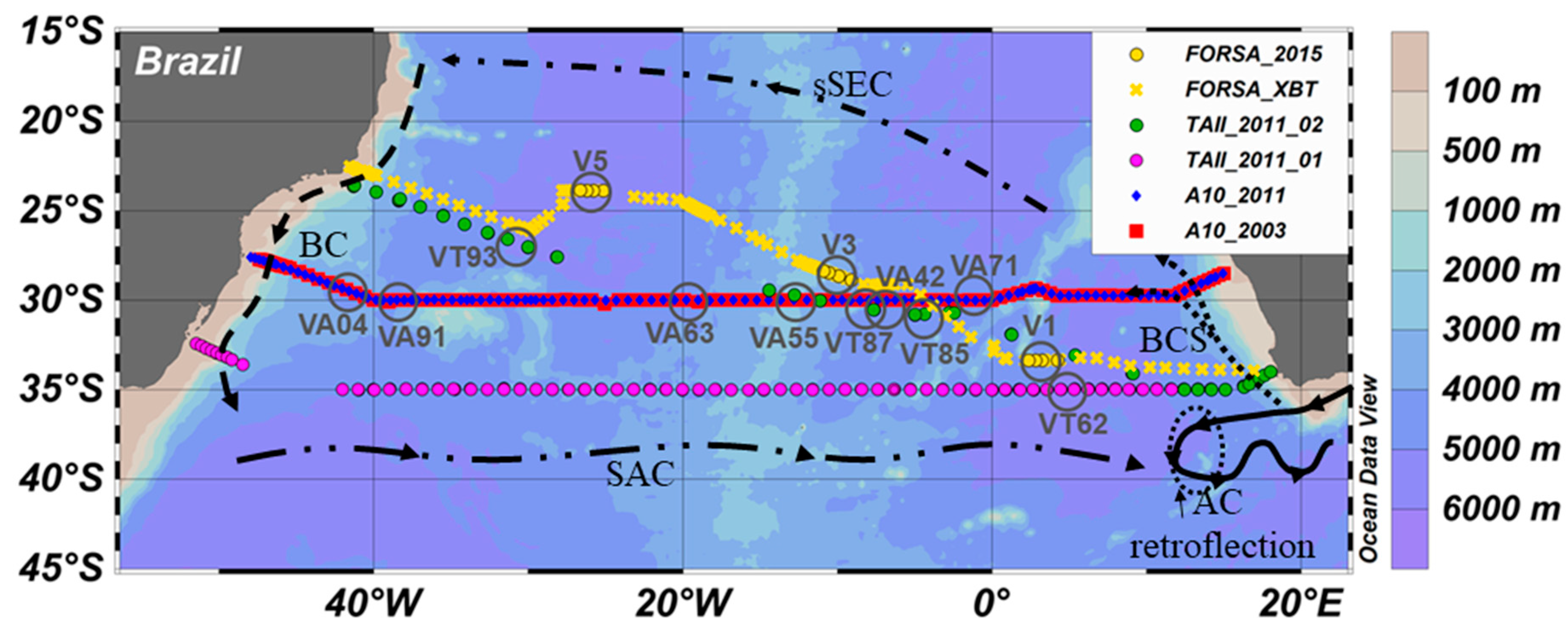
2.1. Cruises Surveys

The Trans-Atlantic II and Following Ocean Rings in the South Atlantic (FORSA) cruises were conducted by the Brazilian High Latitude Oceanography Group (GOAL) [37] in close cooperation with scientists from different research institutions in Brazil (Figure 1). The Trans-Atlantic II (TAII) cruise that occurred in 2011 on board the Brazilian Navy RV NHo Cruzeiro do Sul is a component of the project, “Measurements and modeling of CO2 fluxes in the South Atlantic and Southern Oceans”. The first leg (TAII_01) was conducted from October 24th to November 25th along 35 °S (from Rio Grande, Brazil, to Cape Town, South Africa) [38], and the second leg (TAII_02) was conducted from December 2nd to December 22nd in a Southwestern–Northeastern section (from Cape Town, South Africa, to Rio de Janeiro, Brazil). The FORSA cruise occurred in 2015 on board the Brazilian Navy RV, NPqHo Vital de Oliveira from June 27th to July 15th in a Southwestern-Northeastern section (from Cape Town, to South Africa to Arraial do Cabo, to Brazil) [34,39]. Along these cruise tracks, hydrographic conductivity-temperature-depth (CTD) stations were sampled: 93 in 2011 during the TAII and 12 in 2015 during the FORSA cruise. In addition to physical data, discrete seawater samples were collected for chemical and biological analyses, which included dissolved oxygen (DO), phytoplankton pigments, and dissolved inorganic nutrients, using a combined Sea-Bird CTD/Carrousel 911+system® equipped with 12 five liter and 24 twelve liter Niskin bottles for the TAII and FORSA cruises, respectively. We conducted continuous measurements when crossing six Agulhas eddies during the FORSA cruise [34], but in this work, we present the results from three of them, i.e., those in which CTD stations were performed throughout the water column. The TAII and FORSA datasets are available by request.
The CLIVAR/WOCE Repeat Hydrography Section A10 occurred along 30 °S (Figure 1). In 2003 (A10_2003), the cruise was conducted under the responsibility of JAMSTEC through the project Blue Earth Global Expedition 2003. The A10_2003 was conducted on board the RV Mirai from November 6th to December 5th (from Santos, Brazil to Cape Town, South Africa) [40]. In 2011 (A10_2011), the cruise was funded by NOAA-OGP and NSF-OCE through the U.S. CLIVAR/CO2/hydrography/tracer program. The A10_2011 cruise was conducted on board the RV Ronald H. Brown from September 26th to October 31th (from Cape Town, South Africa to Rio de Janeiro, Brazil) [41]. Along the A10 cruises, 110 stations were sampled in 2003 and 120 in 2011. Physical data and discrete seawater samples were collected for chemical analysis. Using a combined Sea–Bird CTD/Carrousel 911+system® equipped with 35 twelve liter and 24 ten/eleven liter Niskin bottles, in the A10_2003 and A10_2011 cruises, the following properties were determined: salinity, DO, dissolved inorganic nutrients, and carbonate system (total dissolved inorganic carbon—CT; total alkalinity—AT; pH). The A10 datasets analyzed during the current study are available from the NODC/NOAA data center (https://www.nodc.noaa.gov/ocads/oceans/RepeatSections/clivar_a10.html).

2.2. Identification of the Agulhas Eddies

During the FORSA cruise, eddy identification was conducted by analyzing the daily Sea Level Anomaly (SLA) data in conjunction with the temperature profiles obtained by high-resolution spatially distributed XBT deployments. Once the eddies were found, water sampling was performed inside and outside of them (see Carvalho et al. [39] for details). The FORSA cruise was the only one previously planned to sample the Agulhas eddies, and, therefore, we needed to identify the eddies sampled in all of the other cruises, as well as their positions. Therefore, we used the mesoscale eddy AVISO product (downloaded from https://www.aviso.altimetry.fr/en/data/products/value-added-products/global-mesoscale-eddy-trajectory-product.html, last data from January 6th, 2017) [42,43]. Eddy identification in the TAII and A10 cruises was performed by looking for the CTD station positions in the SLA field of the day, in which the station was performed. In cases of an anticyclonic eddy (positive SLA) matching the station position, the back trajectory was investigated to determine whether it could be considered an Agulhas eddy or not. In positive cases, the life history of the eddy was used to determine its mean radius (km) and lifetime (days, d), as well as the sampled day’s radius and age (Table 1), according to the AVISO product, as performed by Orselli et al. [34]. The track of each cruise and the position of the identified eddies in the South Atlantic Ocean are presented in Figure 1.

2.3. Carbonate System Sampling and Analysis

2.3.1. A10_2003 Cruise

The seawater samples for CT were collected into 300 mL borosilicate glass bottles, which were fixed with 100 µL of a saturated mercuric chloride solution [44]. Analysis was performed with two CT measurement systems (systems A and B; Nippon ANS, Inc.) composed of a CO2 extraction system and a coulometer (Model 5012, UIC Inc.), following Johnson et al. [45]. The systems were calibrated using Na2CO3 solutions (nominally 500, 1000 1500, 2000, and 2500 µmol L−1) [46] and analysis of certified reference material (CRM, batch 60, provided by Prof. A. G. Dickson of Scripps Institution of Oceanography). The standard deviations of CRM-CT for systems A and B were 1.1 and 0.9 µmol kg−1 (n = 35; n = 28), respectively. For AT, the samples were collected into 130 mL borosilicate glass bottles. Analyses were conducted with a Metrohm autoburette and a Thermo Orion pH meter, which were automatically controlled. The system was calibrated using 5 solutions of Na2CO3 in 0.7 M NaCl solutions (nominally 0, 100, 1000, 2000, and 2500 µmol kg−1), as well as analysis of CRM (batch 60). The standard deviation of CRM-AT for the system was 1.7 µmol kg−1 (n = 162). The cruise report supplies detailed information on these systems and analysis processes [40].

2.3.2. A10_2011 Cruise

The seawater samples for CT were collected into precombusted 300 mL Pyrex bottles, which were fixed with 0.122 mL of a 50% saturated mercuric chloride solution. Analysis was conducted with two CT measurement systems (PMEL-1 and PMEL-2) composed of a coulometer (UIC Inc.) and a SOMMA (Single Operator Multiparameter Metabolic Analyser) inlet system, following Johnson et al. [47,48] and Johnson [49]. The systems were calibrated using pure CO2 (99.995%) and secondary standards, as well as the analysis of CRM (batch 98). The CT error was not included in the cruise report. For AT, the samples were collected into 500 mL borosilicate glass bottles. Analysis were performed with a Metrohm 665 Dosimat titrator and an Orion 720A pH meter. The system was calibrated using CRM (batches 96 and 112). The reported error for AT was 0.3 µmol kg−1. The cruise report supplies detailed information on the systems and analysis processes [41].

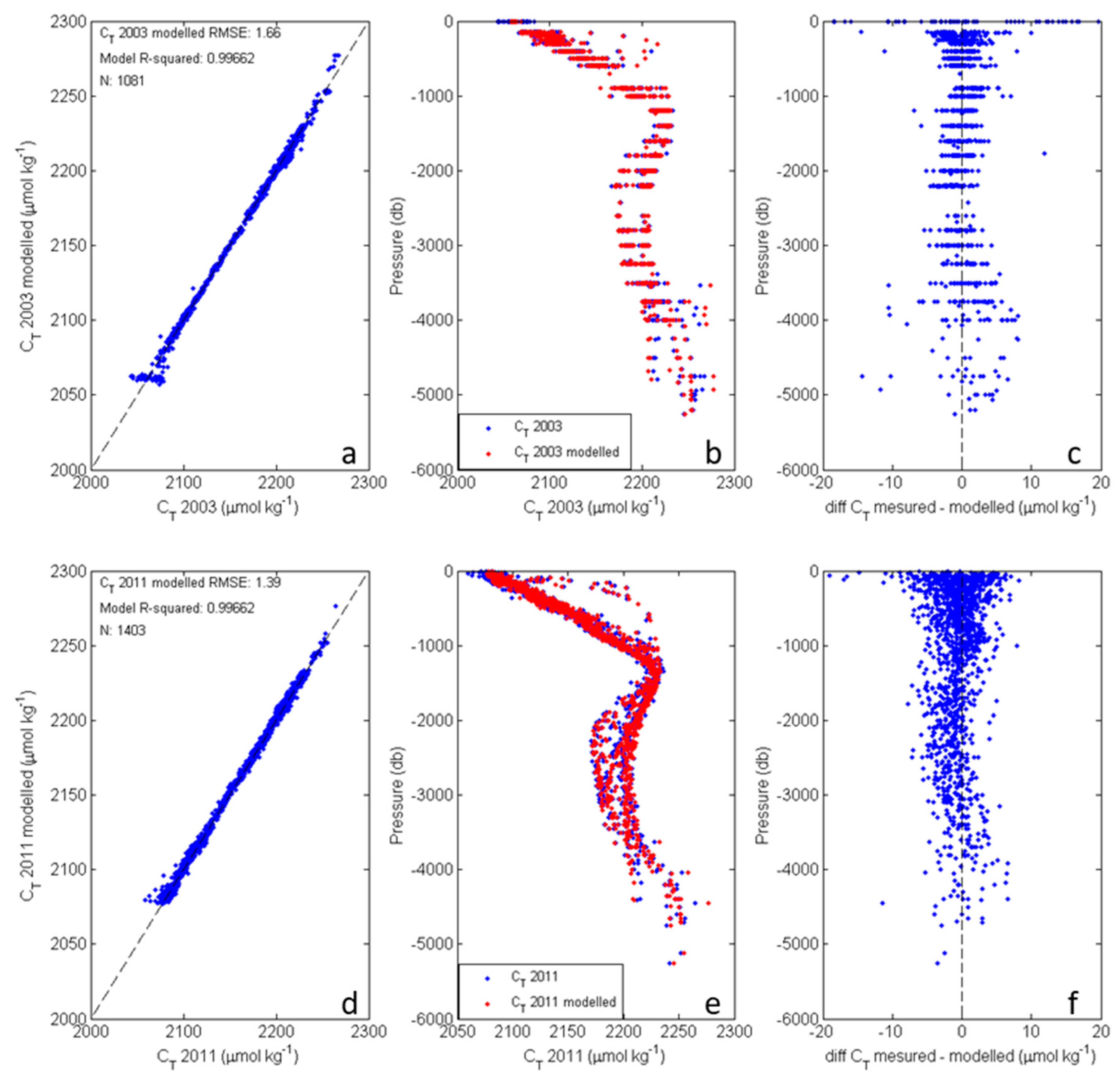
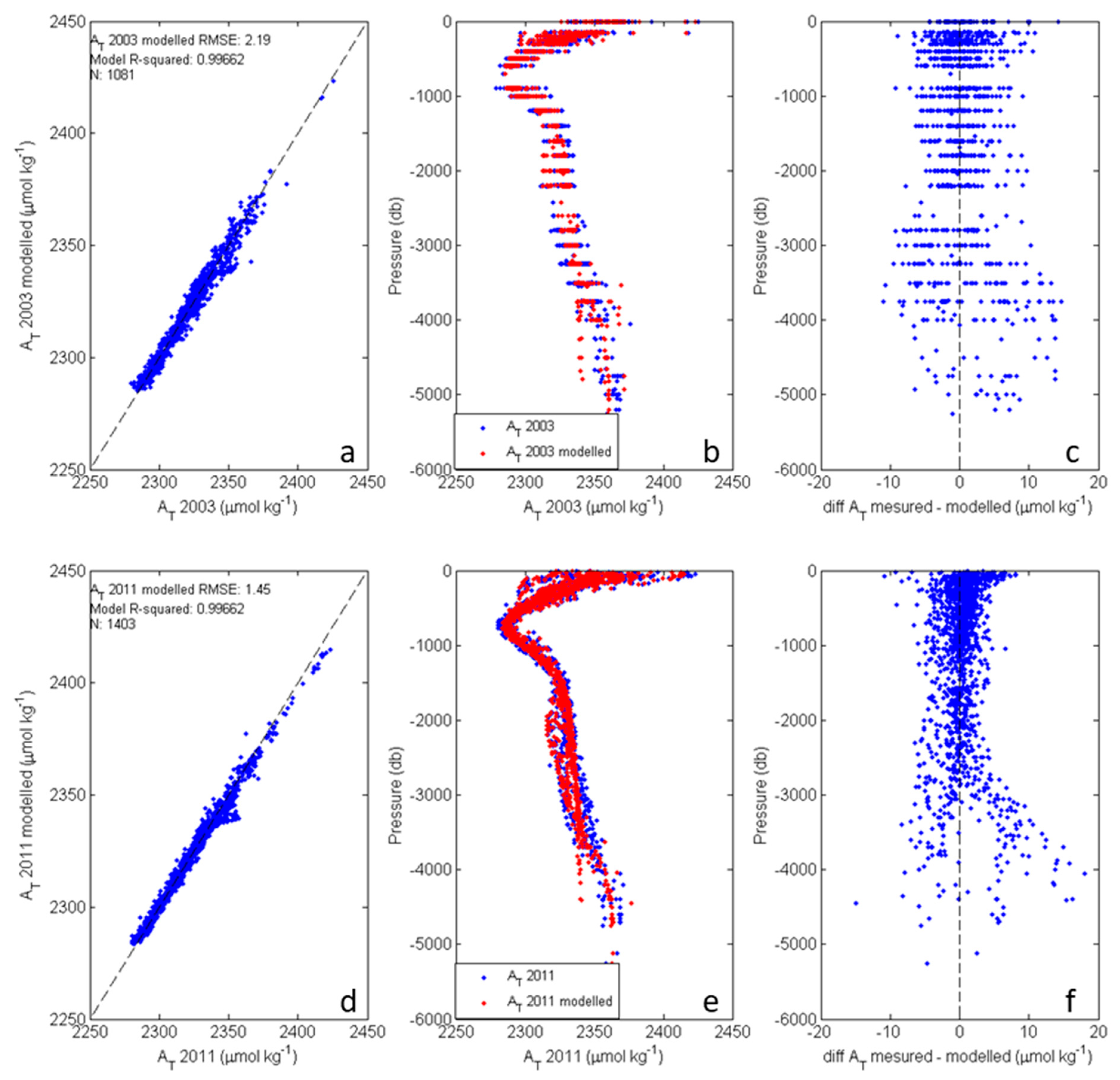
2.4. Polynomial Model Development for Carbonate System Parameters

To gather the carbonate system data along all of the cruise sections investigated in this work, polynomial models for CT and AT parameters were developed using the two A10 sections in which accurate biogeochemical data were available with good precision [40,41]. We chose to use only potential temperature (θ), salinity, and apparent oxygen utilization (AOU) to develop the models, allowing us to apply the models with the greatest number of data as possible, because this approach facilitated the reconstruction of CT and AT in all stations and depths where thermohaline properties were available.
The models were developed through polynomial equations introduced in this work and have the following form (Equation (1)):
f ( x , y ) = i = 0 , j = 0 5 , 5 i p i j x i y j
where f represents the CT or AT functions (μmol kg−1), x is the potential temperature (θ°C) for both CT and AT equations, y is the apparent oxygen utilization (AOU μmol kg−1) for the CT equation, and the salinity for the AT equation, x and y are standardized by the mean and standard deviations, and Pij are the coefficients determined in this model (presented in Table 2). Specifically, i and j are the indices that indicate the exponent of the parameters corresponding to x and y in Equation (1). These polynomial models were subsequently applied to the dataset of the hydrographic sections of the TAII and FORSA cruises.
We tested different types of models to find the one that best represented the biogeochemical data and produced the smallest associated errors. These tests were also performed with the multilinear regression models, because they are commonly applied to carbonate system data reconstruction. In our study, we ultimately chose nonlinear regression, because the best fit to the A10 data was obtained with the polynomial models introduced in this work (Equation (1), Table 2). These models were developed using the curve fitting tool toolbox of MATLAB ®, with the least absolute residual mode. This option considered all data as important, minimized the residuals, and can be used when the data series have few nonconfinable values [50].

2.5. Anthropogenic Carbon Estimate

Considering that CO2 can be continuously exchanged across the ocean–atmosphere interface and absorbed/produced by biological activity in the ocean photic layer (i.e., the carbon reservoirs are not in equilibrium), it is believed that the carbon permanently taken up by the ocean is below the surface mixed layer, where it can be split into natural and anthropogenic origin. Thus, the lower limit of the surface mixed layer is the upper ocean boundary, which is used to define the region in which the Cant content can be estimated [51]. Therefore, in this work, we considered quantifying the Cant below 200 m depth, excluding the surface mixed layer data e.g., [52].
We applied the Tracer combining Oxygen, inorganic Carbon, and total Alkalinity (TrOCA) method to estimate the Cant (Cant-TrOCA) [52,53,54]. In our calculations, we used the CT and AT obtained either from in situ measurements or the model results for all South Atlantic Ocean sections. In addition, we decided to fix the Cant content estimated in the 2003 cruise as a reference to calculate the Cant content difference between the cruise years (ΔCant-TrOCA 2011–2003). Additionally, using the CT model developed for the A10 cruises and applied in all the cruise sections, the CT content difference between years was determined (ΔCT 2011–2003). Considering the year of the cruise, we used the 2011 coefficients to apply for the TAII–2011 cruise data to evaluate the snapshot period of this sampling moment. For the FORSA–2015 cruise, we assumed a linear change between 2003 and 2011 and we added half of this CT difference to derive the CT increase between 2011 and 2015. In this way, we evaluated the Cant content for the entire industrial period (Cant-TrOCA) and compared the Cant and CT differences between 2011 and 2003 (2015 and 2003, for the FORSA cruise section).

3. Results

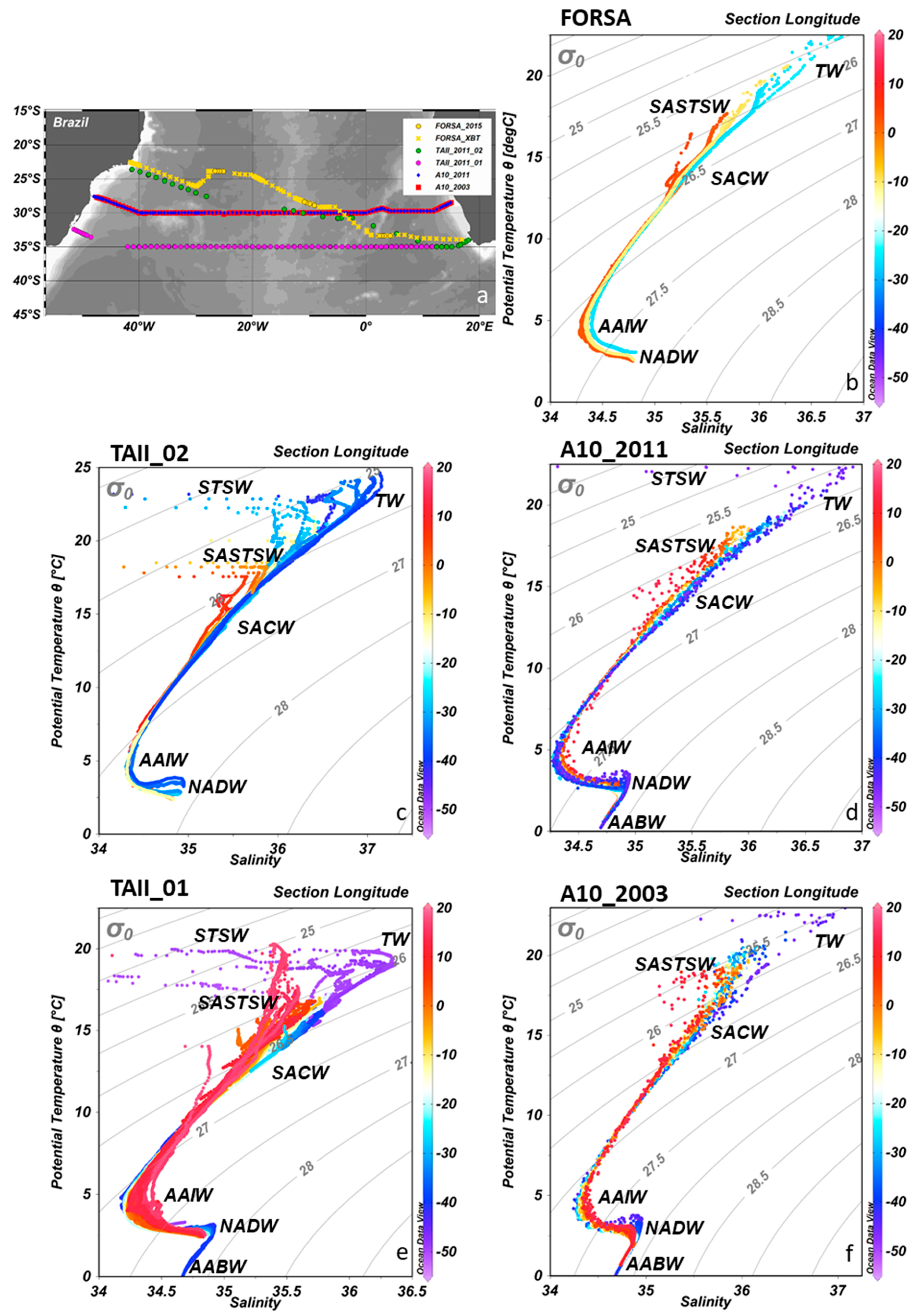
3.1. Physical Structure and Hydrographic Properties along the Cruise Tracks

The differences of the salinity and temperature distribution among the sections are presented in the vertical profiles and θ/S-longitude diagrams (Figure 2 and Figure 3), and the thermohaline properties of the water masses are included in Table 3. Close to the Brazilian coast, the Subtropical Shelf Water (STSW) is observed in the surface of the TAII_01, TAII_02, and A10_2011 cruise sections. TW is observed in the surface in the Western side of all sections. The South Atlantic Subtropical Surface Water (SASTSW) [38,55], which is fresher and colder than the TW, was observed along the TAII_01 section and in the Eastern side of the other sections. The difference in temperature between the Eastern and Western basins for both the FORSA and TAII_02 cruises was stronger than the others because of the Southeast–Northwest direction of the sections (Figure 2 and Figure 3). The SACW and AAIW were identified in the central and intermediate layers, respectively, in all sections. The former is marked by a wide range of temperature and salinity, and the latter has a narrow variation of these parameters, because it is also fresher and colder. We were not able to observe the uCDW in the cruise sections, although previous studies have found it [23]. The NADW, which presented saltier and colder characteristics compared to AAIW, was identified immediately below the AAIW e.g., [24].

3.2. Polynomial Models for Carbonate System Parameters

The polynomial models introduced in this work (Equation (1), Table 2), have the smallest standard deviations from the in situ data and the best precision for both CT and AT data (Figure 4 and Figure 5). The CT models presented root mean square error (RMSE) values of 1.66 μmol kg−1 (r2 = 0.997, n = 1081, p < 0.05) and 1.39 μmol kg−1 (r2 = 0.997, n = 1445, p < 0.05), whereas AT presented RMSE values of 2.19 μmol kg−1 (r2 = 0.983, n = 1081, p < 0.05) and 1.45 μmol kg−1 (r2 = 0.984, n = 1445, p < 0.05), for 2003 and 2011, respectively (Figure 4 and Figure 5). The low RMSE values demonstrated that the developed models were able to correctly represent the CT and AT parameters throughout the entire water column. The errors reported are within the values determined by the Global Ocean Acidification Observing Network (GOA-ON) as climate precision (i.e., estimated within an uncertainty of approximately 2 µmol kg−1 in measurements of CT and AT) [57]. Some differences between the measured and modeled data were found at the sea surface due to the influence of abiotic processes and gas transfer at the sea-air interface (uptake/release), as well as water masses mixing with different CO2 sources e.g., [52,58]. However, the data above the surface mixed layer were not used. These models were developed in the region of the South Atlantic gyre. Thus, they can be used for CT and AT reconstruction in the South Atlantic Ocean when considering the follow ranges of input data: 0 < T (°C) < 25; 33.5 < S < 37.5; 92 < DO (μmol kg−1) < 265.

3.3. Anthropogenic Carbon Content

We present the Cant-TrOCA because it indicates the Cant content in the water column in all sections and eddies at their sample times (Figure 6). For the A10 cruises, the Cant-TrOCA was estimated using the measured concentrations and not the modeled values because they were used to develop the biogeochemical models. In addition, the differences between ΔCant–TrOCA and ΔCT for the cruise years (Figure 7) clearly indicate that the TrOCA method could reliably identify the Cant content. This dissimilarity could be due to the existing interannual variability of thermohaline properties, because the TrOCA method considers the physical structure of the water column (i.e., AT, S and θ) and not only the CT content. Moreover, the AT is not affected by Cant e.g., [59,60], so it can perfectly indicate the physical variation among years, because it is a parameter related to salinity [61]. This is an important point because we focus on the Agulhas eddies, which are mesoscale structures with significant hydrographical differences between their interior and surrounding waters e.g., [62]. Because we consider the Cant concentrations at a large latitudinal range (22 °S–35 °S), these values reflect the large hydrographic differences in temperature and salinity fields (as observed by comparing the panels of Figure 2 and Figure 3). Additionally, the error propagation equations e.g., [4,5,53,63] was used to determine the precision of the Cant_TrOCA method. To perform this analysis, we used the physical parameter measurement (θ, S) uncertainties together with the CT/AT estimation uncertainties, achieving values ranging from 2.82 to 3.83 µmol kg−1 for the application of 2011 and 2003 CT/AT precision, respectively. Compared with the precision of CT (1.39 and 1.66 µmol kg−1 for 2011 and 2003, respectively), these estimates allowed us to conclude that they are of the same order of magnitude and are also smaller than the previous reports from other Cant methods (e.g., ~5–6 µmol kg−1 for TrOCA [4,5,63] and ~10 µmol kg−1 for ΔC* [64]).

3.4. Characteristics and Physical-Chemical Structure of the Agulhas Eddies

Investigation of the Agulhas eddies was not the focus in three of four cruises studied in this work (i.e., in four of the five sections). As a consequence, certain eddies were not necessarily sampled close to their centers but only crossed at their borders (i.e., VA55, VA63, VT85, and VT87). Thus, the sections of temperature, salinity and Cant of each of these eddies do not always show a typical eddy profile. However, at least a minor signal of an eddy profile can be observed in all eddy sections, apart from the SLA used in their identification. Accordingly, a typical thermostad and/or halostad was observed in the sections of those structures. We present the Cant-TrOCA profile of each eddy and the surrounding waters in Figure 8. Comparing the Cant content (± standard deviation) inside and outside the eddies, this value was significantly higher (23% ± 14%) inside all the structures than the value at the same depth in the surrounding waters. A general overview of this difference can be observed in the entire cruise sections (Figure 6), and a more detailed view of the inside–outside Cant sections focused on each of the sampled eddies (Figure 8 and Figure 9). Considering the inside–outside difference at 500 m depth, the mean Cant inside was 18% ± 12% higher than that outside and reached 29% ± 15% at 1000 m depth (Figure 9).
The radius and age of each studied eddy, with consideration of (i) the sampled day and (ii) the life history, are included in Table 1, which indicates that the eddies were sampled at different stages of their lives. We did not observe a relation between the Cant content according to their respective age, radius in the sampled day, or the sampled basin (Eastern/Western). However, we observed certain relatively old eddies (VA04, VA91, and VT93) near the Brazilian coast, which are, therefore, prone to merge with the Brazilian Current and impact the coastal/shelf ecosystems [65].

4. Discussion

4.1. Polynomial Models for Carbonate System Parameters

The polynomial models introduced in this study were able to correctly represent CT and AT with GOA-ON climate precision (i.e., estimated within an uncertainty of approximately 2 µmol kg−1 in measurements of CT and AT) [57], because the achieved RMSE values were smaller than 1.66 μmol kg−1 for CT and 2.19 μmol kg−1 for AT (Figure 3 and Figure 4). Additionally, the results obtained using the polynomial models developed in this work presented a smaller RMSE than those observed for previous model studies e.g., [66]. For AT, for example, the polynomial models introduced here presented a RMSE that was reduced by a factor of 2 compared to the RMSE reported by Carter et al. [66] when using only θ and S: 2.19 and 1.45 μmol kg−1 (this study—2003 and 2011, respectively) versus 4.4 μmol kg−1 [66]. The same result was observed when we compared our results with those of Goyet et al. [50] for both AT and CT. These differences could be related to the fact that these authors [50,66] were considering global oceans (i.e., larger scales) in their studies. The CT RMSE determined in this study are in good agreement with the results reported by Goyet & Davis [58], who presented an uncertainty of 2 μmol kg−1 versus 1.66 and 1.39 μmol kg−1 (2003 and 2011, respectively) in their work.
In addition, the uncertainties observed in the models developed in this study are similar to the reported precision of direct carbonate parameter measurements e.g., [35,59] and have the same order of magnitude indicated in the guide of best practices for CO2 measurements [44] using the recommended equipment and analysis. Furthermore, the GOA-ON reinforces the importance of the construction of biogeochemical databases with climate precision as good as what we have achieved [57]. Thus, these polynomial models are considered robust for CT and AT reconstruction in the South Atlantic basin and can contribute to filling the spatiotemporal gaps and allow reconstruction of marine carbonate system parameters with small uncertainties in the South Atlantic Ocean e.g., [67].

4.2. Anthropogenic Carbon Content in the South Atlantic Ocean

Comparing our Cant estimates with the recent study of Gruber et al. [7], we note that our results were relatively higher than theirs. One main explanation for this difference is related to the Cant methods. This type of difference is normally expected. These differences could also be related to the fact that the previous studies researched the Cant uptake of an early period between 1994 and 2007 (13 years), whereas we investigated the uptake between 2003 and 2011 (8 years) and from 2003 to 2015 (12 years). Additionally, we performed another type of investigation, which was our main focus, i.e., a Cant estimate for the entire industrial period. For the subtropical South Atlantic Ocean, Gruber et al. [7] found a range from 14 to 16 μmol kg−1 corresponding to the central layer (neutral density of 26.60 kg m−3, ~400 m; subtropical mode waters layer), whereas we found values ranging from 18 to 35 μmol kg−1 (30 to 40 μmol kg−1) for the period of 2003 to 2011 in the TAII_01 longitudinal section (2011 and 2015 in the FORSA Southeast–Northwest section) at the same layer. As expected, the central layer corresponding to the Southeast–Northwest section is more significantly affected by the Cant. Previous studies [4,5] have reported that the central waters of the Western South Atlantic Ocean are more significantly affected by the Cant penetration than the waters corresponding to the layers above and below, which is reflected in the faster acidification rate of the SACW [4,5].
Looking at the intermediate layer (neutral density of 27.40 kg m−3, ~1000 m; AAAIW layer in the South Atlantic Ocean), the same authors found a range that varies from 5 to 8 μmol kg−1, whereas we found values ranging from 15 to 22 μmol kg−1 (13 to 18 μmol kg−1) for the period of 2003 to 2011 in the TAII_01 longitudinal section (2011 to 2015 in the FORSA Southeast-Northwest section) at the same layer. The slightly higher values of the TAII_01 longitudinal section can be justified by the fact that this sampling was performed along 35 °S, which is closer to the Antarctic Intermediate Water formation region.
Comparing our study with previous work that used the same methodology in the South Atlantic Ocean [4,5], the findings related to the Cant content in the water column since the industrial revolution are in agreement. For the both SACW and AAIW, the results observed in this work are inside the range observed for the shelf-break region of the Brazilian coast [4] as well as for the Argentine Patagonian zone [5].
Additionally, we aimed to compare the Cant content estimated by the TrOCA method between cruise years (ΔCant-TrOCA 2011–2003) and a simple CT difference between cruise years (ΔCT 2011–2003) at different cruise sections. Thus, we compared the results for the FORSA Southeast–Northwest section (Figure 7a,b) and for the TAII_01 longitudinal section (Figure 7c,d; i.e., one comparison between Figure 7a,b and another between Figure 7c,d). With respect to method comparison, we found that the difference is small, indicating that the TrOCA method could reliably identify the Cant content. The Cant amount found in this peak, approximately 800 m (observed in plots c and d), was observed near the South Brazilian coast, a region that was sampled only in the TAII cruise and not in the FORSA cruise. As indicated by other studies e.g., [4,5], the central layer of this region is more significantly affected by Cant penetration than the layers below and above. Thus, we believe that this difference is reasonable.

4.3. Role Played by the Agulhas Eddies in Anthropogenic Carbon Transport in the South Atlantic Ocean

Considering that the Agulhas eddies can intensify the CO2 uptake at the sea surface compared to the surrounding waters [34], more Cant can penetrate into the water column through the mode water formation processes. Because SACW is composed of several varieties of South Atlantic mode waters [20,33] and receive a considerable input of Indian mode waters [20], the propagation of the Agulhas eddies within the South Atlantic Ocean could be one of the key processes responsible for the rapid acidification levels reported for the central waters of this basin [3,4,5]. This hypothesis is proven by the greater amounts of Cant found inside the eddies than in their surrounding waters (Figure 8 and Figure 9). On average, the Cant content is 18% (29%) higher in the waters inside the eddy at 500 m (1000 m) than outside at the same depth (Figure 9).
It is important to reiterate that each eddy has its own physical characteristics, leading to different intensities on their physical forces. The larger the eddy diameter is after its formation, the greater its expected lifetime. As shown in Table 1, the VA04 eddy is the largest structure used in this study, with a radius of approximately 130 km on its sampling day and a mean radius during its lifetime of approximately 111 km. These physical spatial differences mean that specific eddies have particularities and make only one third of them capable of reaching the Western boundary of the South Atlantic Ocean [68,69]. Reinforcing the most important landmarks for the eddy lifetimes, one portion of the Agulhas eddies can die while crossing the Walvis Ridge, while another portion can die while crossing the Mid-Atlantic Ridge. Additionally, these eddies can suffer splitting and merging processes during their trajectories, as we observed for i) V5 in our previous study [34], in which we identified and interaction between V4 and V5 and V5 and V6, and for ii) VA91, which was formed during the splitting of a 925 days old eddy (Table 1). These interactions between eddies are more common when considering the Agulhas evolved eddies (V5 and VA91, for example), which are structures observed on the Western basin of the South Atlantic Ocean after crossing the Mid-Atlantic Ridge [34].
Thus, the Agulhas eddies (i) intensify the CO2 uptake at the sea surface, as shown by Orselli et al. [34]; (ii) can strengthen the formation processes of the mode waters by increasing the heat flux [18,33]; (iii) contain more Cant than their surrounding waters, as suggested by Woosley et al. [70] and also observed in this study; and (iv) can also carry water masses sourced in the Indian Ocean e.g., [28]. These facts indicate that these mesoscale structures could be one of the key processes influencing the South Atlantic Ocean acidification state through transport of both natural and anthropogenic CO2. It is interesting to note that a recent study by Gruber et al. [7] showed that the waters of the subtropical gyre of the South Atlantic Ocean are facing an anomalous increase in the Cant inventory. These observations correspond to the water column content integrated from the surface to 3000 m depth, which is the region under the influence of the Agulhas eddies.
Moreover, in more recent studies, Laxenaire et al. [68] and Guerra et al. [69] observed the physical interaction between some Agulhas eddies and the Brazil Current. Guerra et al. [69] found that over 23 years, one third of the identified Agulhas eddies released in the retroflection zone reached the Western boundary of the South Atlantic Ocean, with an impact on sea surface temperature (SST), sea surface salinity (SSS), and heat content in the South and Southeast Brazilian coast e.g., [71]. These changes in the SST of the Western boundary led to modifications in the precipitation regime, fluvial discharges, and hydrological cycle, thus affecting the Brazilian coast [1,72,73]. Castellanos et al. [74] verified that an increase in the Agulhas leakage influences the precipitation regime and latent heat flux on the Brazilian coast. Additionally, these eddies can cause intensification of the subtropical gyre [3,74] and can also modify the way in which the El Nino Southern Oscillation impacts the entire South America due to atmospheric teleconnections [1,72,73].
Changes in marine life and biogeochemical cycles are also expected [1]. In the first study of the ocean acidification state in the Brazilian margins, Carvalho-Borges et al. [4] observed an acidification rate of −0.0017 yr−1 in the SACW. These authors found that the central and intermediate layers of the Brazilian coastal region are experiencing an acidification rate of the same magnitude as that of the Argentinean Patagonia (−0.0018 yr−1), which is the other coastal region influenced by southward transport along the Southeast South Atlantic Ocean [5]. However, Carvalho-Borges et al. [4] reinforced that this −0.0017 yr−1 value could be underestimated, indicating that the SACW presented in the southwest Atlantic Ocean could be suffering even greater acidification changes than those reported in the central gyre of the South Atlantic Ocean. Previously, Woosley et al. [70] suggested that the Agulhas eddies can carry up to 20% more Cant than the surrounding waters, which is reinforced by this study (≥23%). Some variations of the observed inside-outside differences could be related to the position of the eddy sampling because certain structures were sampled in their centers, and others were sampled closer to their borders.
Previous studies report that the Western basin of the South Atlantic Ocean could be acidified faster than its Eastern basin due to the stronger ventilation processes e.g., [35], or cross-shelf carbon transport e.g., [4]. We demonstrate in this work that the Agulhas eddies often play a key role in the acidification state of the central waters of the South Atlantic Ocean through the transport of 23% more Cant than their surrounding waters. This excess of CO2 reaching the Brazilian coast can also have an influence on sensitive marine ecosystems (e.g., coral reefs, rhodolith beds, and continental shelf areas) along the Western South Atlantic Ocean region, which have ecological and economical importance and are considered nonrenewable resources [1,4,65].

5. Summary and Conclusions

This research focused on the influence of Agulhas eddies on Cant transport through the South Atlantic Ocean and their impact on ocean acidification. We used in situ data from three zonal and two Southeast–Northwest transects obtained during three cruises conducted in the spring of 2003 and 2011 and one in the winter of 2015. During these surveys, 13 Agulhas eddies were sampled with CTD stations. We modeled the carbonate parameters in locations where they were not directly measured in the cruises using the polynomial models introduced in this work, which were considered robust in CT and AT reconstruction. Additionally, we estimated the Cant content in the water column. The Agulhas eddies have a stronger uptake ability than their surrounding waters, thus increasing the atmospheric CO2 sink [34]. A typical Agulhas eddy can take up −2.12 kg CO2 d−1, leading to a −2.08 t CO2 lifetime−1 [34]. In this study, we also showed that the Agulhas eddies contain up to 29% more Cant than their surrounding waters, which could be influenced by the mode water formation processes. Because mode waters compose the SACW e.g., [20,32], which currently acidifies faster than the surface and intermediate layers of the South Atlantic Ocean [3,4,5,6], we concluded that the Agulhas eddies can act as a trigger for the acidification state of the central water layer of the South Atlantic Ocean via the uptake and consequent transport of large amounts of Cant. Furthermore, recent evidence, such as the interaction between the Agulhas eddies and the Brazil Current [68,69], the contribution of Indian Ocean mode waters observed in the South Atlantic Ocean [20], and the increasing Agulhas leakage [29], highlights the need for additional investigation of the impact of eddies on South Atlantic Ocean acidification. In this study, we focus on the importance of Agulhas eddy dynamics in South Atlantic Ocean biogeochemistry, which is an interesting and novel research topic still under development.
Future studies should focus on other ocean processes and quantification of the Agulhas eddies’ impacts on SACW acidification, because the SACW is experiencing intense acidification changes that could have severe impacts on Brazilian coastal ecosystems. These studies should also investigate the global importance of Agulhas eddies in biogeochemistry, because they play an important role in the subtropical gyre of the South Atlantic Ocean and Atlantic meridional overturning circulation [21,71]. Thus, a natural outcome of the results presented in this work is to implement high-resolution process-oriented numerical modeling experiments, including downscaling, which are lacking in current investigations [1,75]. Additionally, we suggest model studies focusing on the impacts of climate change on Agulhas leakage and eddy release, because these phenomena are associated with wind system modifications [29]. Future studies should also focus on its consequences of Agulhas leakage and eddy release on marine organisms and ecosystems.

Author Contributions

I.B.M.O. conducted the data analysis and modeling elements of this study as her PhD project. C.G. acted as the main supervisor for I.B.M.O. in conducting this work and as an expert on carbonate system data and modeling. R.K. acted as a second supervisor for I.B.M.O. in proposing the study and as an expert on carbonate system and water masses. J.L.L.d.A. acted as a third supervisor for I.B.M.O. and as an Agulhas-eddy expert. M.A. contributed as an eddy expert and as P.I. of the FORSA cruise. F.G. conducted the satellite data and AVISO product processing. F.T. contributed as an expert in anthropogenic carbon calculations. C.A.E.G. was the main coordinator for the Brazilian research cruises and was responsible for supplying the TAII and FORSA cruise opportunities for the observations. All authors contributed to the interpretation of results and/or to the writing of the paper.

Funding

This study offers a contribution to the activities of the Brazilian High Latitude Oceanography Group (GOAL) and the Brazilian Ocean Acidification Network (BrOA; www.broa.furg.br). The TAII and FORSA projects were sponsored by the Brazilian National Council for Scientific and Technological Development (CNPq) and Brazilian Improving Coordination of Higher Education Personnel (CAPES), with logistics supported by the Ministry of Science, Technology, Innovation, and Communication (MCTIC), the Brazilian Ministerial Secretary for the Resources of the Sea (SECIRM), and the Brazilian Navy. FORSA was also sponsored by the Brazilian Coastal Monitoring System (SiMCosta). This study also contributes to the project “Estudos Avançados de Médias e Altas Latitudes” (CAPES grant n° 23038.001421/2014-30). I. B. M. Orselli acknowledges CAPES/CMAR2 for her Ph.D. funding (CAPES process n°. 23038.001421/2014-30 and BEX 0077/17-8). R. Kerr acknowledges the CNPq researcher grants nº 302604/2015-4 and 304937/2018-5. M. Araujo in grateful for the support of the Brazilian Research Network on Global Climate Change-Rede CLIMA (FINEP grants 01.13.0353-00).

Acknowledgments

The authors thank all the researchers and students from LEOC/FURG and LOFEC/UFPE for their contributions to cruise planning and sampling, as well as researchers from IMAGES_ESPACE-DEV/UPVD for discussions and suggestions. The authors also thank the crew of the Brazilian vessels RV NHo Cruzeiro do Sul and RV NPqHo Vital de Oliveira for their logistical assistance. Because this work used the Mesoscale Eddy Trajectory Atlas product, the authors thank its producers, supporters, collaborators and distributers: SSALTO/DUACS, CNES, Oregon State University, NASA and AVISO. We also thank for the availability of the CLIVAR/WOCE Repeat Hydrography Section A10 data. The authors thank the editors and three reviewers for their comments and suggestions, which have significantly improved the manuscript.

Conflicts of Interest

The authors declare that they have no conflicts of interest. The funders had no role in the design of the study; in the collection, analyses, or interpretation of data; in the writing of the manuscript, or in the decision to publish the results.

References

  1. Campos, E.J.D.; França, C.A.S.; Rodrigues, R.R.; Muelbert, J.H. Inter-relações entre o Atlântico Sul, plataforma continental e regiões costeiras do sul e do sudeste do Brasil. In Ciência das Mudanças Climáticas e sua Interdisciplinaridade; Ambrizzi, T., Jacobi, P.R., Dutra, L.M.M., Eds.; Annablume Editora: São Paulo, Brazil, 2015; ISBN 978-85-391-0714-8. [Google Scholar]
  2. Takahashi, T.; Sutherland, S.C.; Wanninkhof, R.; Sweeney, C.; Feely, R.A.; Chipman, D.W.; Hales, B.; Friederich, G.; Chavez, F.; Sabine, C.; et al. Climatological mean and decadal change in surface ocean pCO2, and net sea-air CO2 flux over the global oceans. Deep-Sea Res. II 2009, 56, 554–557. [Google Scholar] [CrossRef]
  3. Salt, L.A.; Heuven, S.M.; Claus, M.E.; Jones, E.M.; Baar, H.J. Rapid acidification of mode and intermediate waters in the southwestern Atlantic Ocean. Biogeosciences 2015, 12, 1387–1401. [Google Scholar] [CrossRef] [Green Version]
  4. De Carvalho-Borges, M.; Orselli, I.B.M.; de Carvalho Ferreira, M.L.; Kerr, R. Seawater acidification and anthropogenic carbon distribution on continental shelf and slope of the western South Atlantic Ocean. J. Mar. Syst. 2018. [Google Scholar] [CrossRef]
  5. Orselli, I.B.M.; Kerr, R.; Ito, R.G.; Tavano, V.M.; Mendes, C.R.B.; Garcia, C.A.E. How fast is the Patagonian shelf-break acidifying? J. Mar. Syst. 2018, 178, 1–14. [Google Scholar] [CrossRef]
  6. Kitidis, V.; Brown, I.; Hardman-Mountford, N.; Lefèvre, N. Surface ocean carbon dioxide during the Atlantic Meridional Transect (1995–2013): Evidence of ocean acidification. Prog. Oceanogr. 2017, 158, 65–75. [Google Scholar] [CrossRef]
  7. Gruber, N.; Clement, D.; Carter, B.R.; Feely, R.A.; van Heuven, S.; Hoppema, M.; Ishii, M.; Key, M.R.; Kozyr, A.; Lauvset, S.K.; et al. The oceanic sink for anthropogenic CO2 from 1994 to2007. Science 2019, 363, 1193–1199. [Google Scholar] [CrossRef] [PubMed]
  8. Howes, E.L.; Joos, F.; Eakin, M.; Gattuso, J.-P. The Oceans 2015 Initiative, Part I: An Updated Synthesis of the Observed and Projected Impacts of Climate Change on Physical and Biological Processes in the Oceans; Studies N°02/15; IDDRI: Paris, France, 2015; p. 52. ISSN 2258-7535. [Google Scholar]
  9. Pardo, P.C.; Pérez, F.F.; Khatiwala, S.; Ríos, A.F. Anthropogenic CO2 estimates in the Southern Ocean: Storage partitioning in the different water masses. Prog. Oceanogr. 2014, 120, 230–242. [Google Scholar] [CrossRef]
  10. Sabine, C.L.; Feely, R.A.; Gruber, N.; Key, R.M.; Lee, K.; Bullister, J.L.; Wanninkhof, R.; Wong, C.S.; Wallace, D.W.; Tilbrook, B.; et al. The Ocean Sink for Anthropogenic CO2. Science 2004, 305, 367–371. [Google Scholar] [CrossRef]
  11. Tanhua, T.; Hoppema, M.; Jones, E.M.; Stöven, T.; Hauck, J.; Dávila, M.G.; Santana-Casiano, M.; Álvarez, M.; Strass, V.H. Temporal changes in ventilation and the carbonate system in the Atlantic sector of the Southern Ocean. Deep-Sea Res. II 2016. [Google Scholar] [CrossRef]
  12. Cox, P.M.; Betts, R.A.; Jones, C.D.; Spall, S.A.; Totterdell, I.J. Acceleration of global warming due to carbon-cycle feedbacks in a coupled climate model. Nature 2000, 408, 184–187. [Google Scholar] [CrossRef]
  13. Touratier, F.; Goyet, C.; Houpert, L.; de Madron, X.D.; Lefèvre, D.; Stabholz, M.; Guglielmi, V. Role of deep convection on anthropogenic CO2 sequestration in the Gulf of Lions (northwestern Mediterranean Sea). Deep-Sea Res. I 2016, 113, 33–48. [Google Scholar] [CrossRef]
  14. Orsi, A.H.; Johnson, G.C.; Bullister, J.L. Circulation, mixing and production of Antarctic bottom water. Prog. Oceanogr. 1999, 43, 55–109. [Google Scholar] [CrossRef]
  15. Rintoul, S. The Southern Ocean in the Earth System; Smithsonian Institution Scholarly Press: Washington, DC, USA, 2011. [Google Scholar] [CrossRef]
  16. Talley, L.; Pickard, G.; Emery, W.; Swift, J. Descriptive Physical Oceanography: An Introduction; Elsevier: Boston, MA, USA, 2011. [Google Scholar]
  17. Emery, W.J. Water types and water masses. In Ocean Circulation; Elsevier: Amsterdam, The Netherlands, 2003; pp. 1556–1567. ISBN 978-0-12-391851-2. [Google Scholar]
  18. Hanawa, K.; Talley, L.D. Mode Waters. In Ocean Circulation and Climate: Observing and Modelling the Global Ocean; Siedle, G., Church, J., Gould, J., Eds.; Academic: San Diego, CA, USA; London, UK, 2001; pp. 373–386. ISBN 0-12-641351-7. [Google Scholar]
  19. Van Aken, H.M.; van Veldhoven, A.K.; Veth, C.; De Ruijter, W.P.M.; van Leeuwen, P.J.; Drijfhout, S.S.; Whittle, C.P.; Rouault, M. Observations of a young Agulhas ring, Astrid, during MARE in March 2000. Deep-Sea Res. II 2003, 50, 167–195. [Google Scholar] [CrossRef]
  20. Souza, A.G.Q.; Kerr, R.; Azevedo, J.L.L. On the influence of Subtropical Mode Water on the South Atlantic Ocean. J. Mar. Syst. 2018, 185, 13–24. [Google Scholar] [CrossRef]
  21. Beal, L.M. A Time Series of Agulhas Undercurrent Transport. J. Phys. Oceanogr. 2009, 39, 2436–2450. [Google Scholar] [CrossRef]
  22. Biastoch, A.; Durgadoo, J.V.; Morrison, A.K.; van Sebille, E.; Weijer, W.; Griffies, S.M. Atlantic multi-decadal oscillation covaries with Agulhas leakage. Nat. Commun. 2015, 6, 10082. [Google Scholar] [CrossRef] [Green Version]
  23. Stramma, L.; England, M. On the Water masses and mean circulation of the South Atlantic Ocean. J Geophys. Res. 1999, 104, 20863–20883. [Google Scholar] [CrossRef]
  24. Ferreira, M.L.; Kerr, R. Source water distribution and quantification of North Atlantic Deep Water and Antarctic Bottom Water in the Atlantic Ocean. Prog. Oceanogr. 2017, 153, 66–83. [Google Scholar] [CrossRef]
  25. Robinson, A.R. Eddies in Marine Science; Springer: Berlin, Germany, 1983; 614p. [Google Scholar]
  26. Biastoch, A.; Böning, C.W.; Lutjeharms, J.R.E. Agulhas leakage dynamics affects decadal variability in Atlantic overturning circulation. Nature 2008, 456, 489–492. [Google Scholar] [CrossRef]
  27. De Ruijter, W.P.; Biastoch, A.; Drijhout, S.S.; Lutjeharms, J.R.; Matano, R.; Pichevin, T.; van Leeuwen, P.J.; Weijer, W. Dynamics, estimation and impact of South Atlantic interocean exchange. J. Geophys. Res. 1999, 104, 20885–20910. [Google Scholar] [CrossRef]
  28. Lutjeharms, J.R.E. The Agulhas Current; Springer: Berlin/Heidelberg, Germany, 2006. [Google Scholar] [CrossRef]
  29. Biastoch, A.; Böning, C.W.; Schwarzkopf, F.U.; Lutjeharms, J.R.E. Increase in Agulhas leakage due to poleward shift of southern hemisphere westerlies. Nature 2009, 462, 495. [Google Scholar] [CrossRef] [PubMed]
  30. Souza, J.M.; de Boyer Montégut, C.; Cabanes, C.; Klein, P. Estimation of the Agulhas ring impacts on meridional heat fluxes and transport using ARGO floats and satellite data. Geophys. Res. Lett. 2011, 38, L21602. [Google Scholar] [CrossRef]
  31. Bard, E.; Rickaby, R.E.M. Migration of the subtropical front as a modulator of glacial climate. Nature 2009, 460, 380–383. [Google Scholar] [CrossRef] [PubMed]
  32. Sato, O.T.; Polito, P. Observation of South Atlantic subtropical mode Waters with Argo profiling float data. J. Geophys. Res. Oceans 2014, 119, 2860–2881. [Google Scholar] [CrossRef]
  33. Villas Bôas, A.B.; Sato, O.T.; Chaigneau, A.; Castelão, G.P. The signature of mesoscale eddies on the air-sea turbulent heat fluxes in the South Atlantic Ocean. Geophys. Res. Lett. 2015, 42, 1856–1862. [Google Scholar] [CrossRef]
  34. Orselli, I.B.M.; Kerr, R.; Azevedo, J.L.L.; Galdino, F.; Araujo, M.; Garcia, C.A.E. The sea-air CO2 net fluxes in the South Atlantic Ocean and the role played by Agulhas eddies. Prog. Oceanogr. 2019, 170, 40–52. [Google Scholar] [CrossRef]
  35. Ríos, A.F.; Álvarez-Salgado, X.A.; Pérez, F.F.; Bingler, L.S.; Arístegui, J.; Mémery, L. Carbon dioxide along WOCE line A14: Water masses characterization and anthropogenic entry. J. Geophys. Res. 2003, 108, 3123. [Google Scholar] [CrossRef]
  36. Moreau, S.; Della Penna, A.; Llort, J.; Patel, R.; Langlais, C.; Boyd, P.W.; Matear, R.J.; Phillips, H.E.; Trull, T.W.; Tilbrook, B.; et al. Eddy-induced carbon transport across the Antarctic Circumpolar Current. Glob. Biogeochem. Cycles 2017, 31, 1368–1386. [Google Scholar] [CrossRef]
  37. Mata, M.M.; Tavano, V.M.; Garcia, C.A.E. 15 years sailing with the Brazilian High Latitude Oceanography Group (GOAL). Deep-Sea Res. II 2018, 149, 1–3. [Google Scholar] [CrossRef]
  38. Lencina-Avila, J.M.; Ito, R.G.; Garcia, C.A.E.; Tavano, V.M. Sea-air carbon dioxide fluxes along 35°s in the Atlantic Ocean and adjacent continental shelves. Deep-Sea Res. I 2016, 115, 175–187. [Google Scholar] [CrossRef]
  39. Carvalho, A.C.O.; Mendes, C.R.B.; Kerr, R.; Azevedo, J.L.L.; Galdino, F.; Tavano, V.M. The impact of mesoscale eddies on the phytoplankton community in the South Atlantic Ocean: HPLC-CHEMTAX approach. Mar. Environ. Res. 2019, 144, 154–165. [Google Scholar] [CrossRef] [PubMed]
  40. Uchida, H.; Fukasawa, M.; Murata, A. WHP P6, A10, I3/I4 REVISIT DATA BOOK Blue Earth Global Expedition 2003 (BEAGLE2003); JAMSTEC Publication: Tokyo, Japan, 2005; Volume 1–2. [Google Scholar]
  41. Wanninkhof, R.; Feely, R.; Millero, F.; Carlson, C.; O’Neil Baringer, M.; Macdonald, A.; Johnson, G.; Zhang, J.-Z.; Mordy, C.; Langdon, C.; et al. Carbon Dioxide, Hydrographic, and Chemical Data Obtained during the R/V Ronald H. Brown in the Atlantic Ocean on CLIVAR Repeat Hydrography Section A10 (September 26—October 31, 2011); Carbon Dioxide Information Analysis Center, Oak Ridge National Laboratory, US Department of Energy: Oak Ridge, TN, USA, 2013. [Google Scholar] [CrossRef]
  42. Chelton, D.B.; Schlax, M.G.; Samelson, R.G. Global observations of nonlinear mesoscale eddies. Prog. Oceanogr. 2011, 91, 167–216. [Google Scholar] [CrossRef]
  43. Schlax, M.G.; Chelton, D.B. The “Growing Method” of Eddy Identification and Tracking in Two and Three Dimensions; College of Earth, Ocean and Atmospheric Sciences, Oregon State University: Corvallis, OR, USA, 2016. [Google Scholar]
  44. DOE. Handbook of Methods for Analysis of the Various Parameters of the Carbon Dioxide System in Seawater; Version 2, ORNL/CDIAC-74; Dickson, A.G., Goyet, C., Eds.; DOE: Washington, DC, USA, 1994. [Google Scholar]
  45. Johnson, K.M.; Dickson, A.G.; Eischeid, G.; Goyet, C.; Guenther, P.; Key, R.M.; Millero, F.J.; Purkerson, D.; Sabine, C.L.; Schottle, R.G.; et al. Coulometric total carbon dioxide analysis for marine studies: Assessment of the quality of total inorganic carbon measurements made during the US Indian Ocean CO2 survey 1994–1996. Mar. Chem. 1998, 63, 21–37. [Google Scholar] [CrossRef]
  46. Goyet, C.; Hacker, S.D. Procedure for calibration of a coulometric system used for total inorganic carbon measurements in seawater. Mar. Chem. 1992, 38, 37–53. [Google Scholar] [CrossRef]
  47. Johnson, K.M.; King, A.E.; Sieburth, J.M. Coulometric TCO2 analyses for marine studies: An introduction. Mar. Chem. 1985, 16, 61–82. [Google Scholar] [CrossRef]
  48. Johnson, K.M.; Williams, P.J.; Brandstrom, L.; Sieburth, J.M. Coulometric total carbon analysis for marine studies: Automation and calibration. Mar. Chem. 1987, 21, 117–133. [Google Scholar] [CrossRef]
  49. Johnson, K.M. Operator’s Manual: Single-Operator Multiparameter Metabolic Analyzer (SOMMA) for Total Carbon Dioxide (CT) with Coulometric Detection; Brookhaven National Laboratory: Brookhaven, NY, USA, 1992. [Google Scholar]
  50. Patil, G.P.; Rao, C.R. Handbook of Statistics. v. 12; Environmental Statistics: Amsterdan, The Netherlands, 1994; 927p. [Google Scholar]
  51. Goyet, C.; Healy, R.J.; Ryan, J.P. Global Distribution of Total Inorganic Carbon and Total Alkalinity below the Deepest Winter Mixed Layer Depths; ORNL/CDIAC-127, NDP-076; Carbon Dioxide Information Analysis Center, Oak Ridge National Laboratory, U.S. Department of Energy: Oak Ridge, TA, USA, 2000; p. 40.
  52. Touratier, F.; Azouzi, L.; Goyet, C. CFC-11, ∆C14C and 3H tracers as a means to assess anthropogenic CO2 concentrations in the ocean. Tellus 2007, 59B, 318–325. [Google Scholar] [CrossRef]
  53. Touratier, F.; Goyet, C. Definition, properties, and Atlantic Ocean distribution of the new tracer TrOCA. J. Mar. Syst. 2004, 46, 169–179. [Google Scholar] [CrossRef]
  54. Touratier, F.; Goyet, C. Applying the new TrOCA approach to assess the distribution of anthropogenic CO2 in the Atlantic Ocean. J. Mar. Syst. 2004, 46, 181–197. [Google Scholar] [CrossRef]
  55. Lutjeharms, J.R.E.; Valentine, H.R. Water types and volumetric considerations of the South-East Atlantic upwelling regime. Afr. J. Mar. Sci. 1987, 5, 63–71. [Google Scholar] [CrossRef] [Green Version]
  56. Möller, O.O., Jr.; Piola, A.R.; Freitas, A.C.; Campos, E.J.D. The effects of river discharge and seasonal winds on the shelf off Southwestern South America. Cont. Shelf Res. 2008, 28, 1607–1624. [Google Scholar] [CrossRef]
  57. Newton, J.A.; Feely, R.A.; Jewett, E.B.; Williamson, P.; Mathis, J. Global Ocean Acidification Observing Network (GOA-ON): Requirements and Governance Plan, 2nd ed. 2015. Available online: http://www.goa-on.org/documents/general/GOA-ON_2nd_edition_final.pdf (accessed on 12 June 2019).
  58. Goyet, C.; Davis, D.L. Estimation of TCO2 concentration throughout the water column. Deep-Sea Res. I 1997, 44, 859–877. [Google Scholar] [CrossRef]
  59. Goyet, C.; Ito, R.G.; Touratier, F. Anthropogenic carbon distribution in the eastern South Pacific Ocean. Biogeosciences 2009, 6, 149–156. [Google Scholar] [CrossRef]
  60. Goyet, C.; Coatanoan, C.; Eischeid, G.; Amaoka, T.; Okuda, K.; Healy, R.; Tsunogai, S. Spatial variation of total CO2 and total alkalinity in the northern Indian Ocean: A novel approach for the quantification of anthropogenic CO2 in seawater. J. Mar. Res. 1999, 57, 135–163. [Google Scholar] [CrossRef]
  61. Millero, F.J. The marine inorganic carbon cycle. Chem. Rev. 2007, 107, 308–341. [Google Scholar] [CrossRef]
  62. Casanova-Masjoan, M.; Pelegrí, J.L.; Sangrà, P.; Martínez, A.; Grisolía-Santos, D.; Pérez-Hernández, M.D.; Hernández-Guerra, A. Characteristics and evolution of an Agulhas ring. J. Geophys. Res. Oceans 2017, 122, 7049–7065. [Google Scholar] [CrossRef]
  63. Kerr, R.; Goyet, C.; Cunha, L.C.; Orselli, I.B.M.; Lencina-Avila, J.M.; Mendes, C.R.B.; Carvalho-Borges, M.; Mata, M.M.; Tavano, V.M. Carbonate system properties in the Gerlache Strait, Northern Antarctic Peninsula (February 2015): II. Anthropogenic CO2 and Seawater Acidification. Deep-Sea Res. II 2018. [Google Scholar] [CrossRef]
  64. Gruber, N.; Sarmiento, J.L.; Stocker, T.F. An improved method for detecting anthropogenic CO2 in the oceans. Glob. Biogeochem. Cycles 1996, 10, 809–837. [Google Scholar] [CrossRef]
  65. Kerr, R.; Cunha, L.C.; Kikuchi, R.K.P.; Horta, P.; Ito, R.G.; Muller, M.N.; Orselli, I.B.M.; Lencina-Avila, J.M.; de Orte, M.R.; Sordo, L.; et al. The western South Atlantic Ocean in a high-CO2 world: Current measurement capabilities and perspectives. Environ. Manag. 2016, 57, 740–752. [Google Scholar] [CrossRef]
  66. Carter, B.R.; Feely, R.A.; Williams, N.L.; Dickson, A.G.; Fong, M.B.; Takeshita, Y. Updated methods for global locally interpolated estimation of alkalinity, pH and nitrate. Limnol. Oceanogr. Methods 2017. [Google Scholar] [CrossRef]
  67. Perretti, A.R.; Albergaria-Barbosa, A.C.R.D.; Kerr, R.; Cunha, L.C.D. Ocean acidification studies and the uncertainties relevance on measurements of marine carbonate system properties. Braz. J. Oceanogr. 2018, 66, 234–242. [Google Scholar] [CrossRef]
  68. Laxenaire, R.; Speich, S.; Blanke, B.; Chaigneau, A.; Pegliasco, C.; Stegner, A. Anticyclonic eddies connecting the western boundaries of Indian and Atlantic oceans. J. Geophys. Res. Oceans 2018. [Google Scholar] [CrossRef]
  69. Guerra, L.A.A.; Paiva, A.M.; Chassignet, E.P. On the translation of Agulhas rings to the western South Atlantic Ocean. Deep-Sea Res. I 2018, 139, 104–113. [Google Scholar] [CrossRef]
  70. Woosley, R.J.; Millero, F.; Wanninkhof, R. Rapid Anthropogenic Changes in CO2 and pH in the Atlantic Ocean: 2003–2014. Glob. Biogeochem. Cycles 2016, 30, 70–90. [Google Scholar] [CrossRef]
  71. Lumpkin, R.; Garzoli, S.L. Interannual to Decadal Variability in the Southwestern Atlantic’s Surface Circulation. J. Geophys. Res. Oceans 2003, 116, C01014. [Google Scholar] [CrossRef]
  72. Rodrigues, R.R.; Haarsma, R.J.; Campos, E.J.D.; Ambrizzi, T. The impacts of inter-El Nino variability on the Tropical Atlantic and Northeast Brazil climate. J. Clim. 2011, 24, 3402–3422. [Google Scholar] [CrossRef]
  73. Rodrigues, R.R.; Campos, E.J.D.; Haarsma, R.J. The Impact of ENSO in the South Atlantic Subtropical Dipole Mode. J. Clim. 2015, 28, 2692–2705. [Google Scholar] [CrossRef]
  74. Castellanos, P.; Campos, E.J.D.; Piera, J.; Sato, O.T.; Silva Dias, M.A.F. Impacts of Agulhas Leakage on the Tropical Atlantic Western Boundary Systems. J. Clim. 2017. [Google Scholar] [CrossRef]
  75. Pereira, J.E.; Wainer, I. A mudança do clima e seus impactos no oceano Atlântico Sul em escala regional. In Ciência das Mudanças Climáticas e sua Interdisciplinaridade; Ambrizzi, T., Jacobi, P.R., Dutra, L.M.M., Eds.; Annablume Editora: São Paulo, Brazil, 2015; ISBN 978-85-391-0714-8. [Google Scholar]
Figure 1. Map of the sampled region in the South Atlantic Ocean. The yellow crosses correspond to the expendable bathythermograph (XBT) profiles performed during the Following Ocean Rings in the South Atlantic (FORSA) cruise (FORSA_XBT). The conductivity-temperature-depth (CTD) stations are indicated by yellow dots (FORSA_2015), green dots (Trans-Atlantic II (TAII)_2011_02), purple dots (TAII_2011_01), blue diamonds (A10_2011), and red squares (A10_2003). The gray circles indicate the approximate positions at which the eddies were sampled: V1, V3, and V5 (FORSA_2015); VT62 (TAII_2011_01); VT85, VT87, and VT93 (TAII_2011_02); VA42, VA63, and VA91 (A10_2011); and VA04, VA55, and VA71 (A10_2003). The black lines represent the main currents of the surface circulation, which are the Benguela Current System (BCS, dotted line), southern branch of the South Equatorial Current (sSEC, dot-dashed line), Brazil Current (BC, dashed line) and South Atlantic Current (SAC, dot-dot dashed line). The Agulhas Current (AC, continuous line) and Agulhas Current retroflection zone (black dotted ellipse) are also indicated. The bottom bathymetry is represented by color shadings.
Climate 07 00084 g001
Figure 2. Map of the cruise sections and sampled eddies (a). For a complete description of this map, please see Figure 1. Left panels show the salinity profiles (be), while right panels show potential temperature (°C; fj) profiles. The hydrographic sections are TAII_02–2011 (b,g), TAII_01–2011 (c,h), A10_2011 (d,i) and A10_2003 (e,j). The continuous gray lines or gray dots indicate the position of the CTD stations (at each 1 m for the TAII and FORSA cruises). Temperatures from the XBT of the FORSA–2015 cruise section and CTD stations are indicated by continuous gray lines (f). The sampled eddies are indicated in the hydrographic sections of all cruises by vertical white lines. The water mass positions in the water column are indicated by their acronyms in panels f to j, referring to: Subtropical Shelf Water (STSW), Tropical Water (TW), South Atlantic Subtropical Surface Water (SASTSW), South Atlantic Central Water (SACW), and Antarctic Intermediate Water (AAIW). For details, please see the θ/S diagrams (Figure 3) and the water masses properties (Table 3).
Climate 07 00084 g002
Figure 3. Map of the cruise sections (a). For a complete description of this map, please see Figure 1. θ/S-longitude diagrams for each section (bf). θ/S-longitude of the FORSA–2015 cruise section (b), TAII_02–2011 section (c), A10_2011 section (d), TAII_01–2011 section (e), and A10_2003 section (f). The continuous gray lines represent the isopycnals. The water masses are indicated by their acronyms, referring to: Subtropical Shelf Water (STSW), Tropical Water (TW), South Atlantic Subtropical Surface Water (SASTSW), South Atlantic Central Water (SACW), Antarctic Intermediate Water (AAIW), North Atlantic Deep Water (NADW), and Antarctic Bottom Water (AABW). For details please see the water masses properties (Table 3).
Climate 07 00084 g003
Figure 4. CT model results considering the A10 section of 2003 (ac) and 2011 (df); measured vs. modeled CT (a,d), including the RMSE of the model equation, measured vs. modeled r2, and number of measurements (N); measured (blue dots) and modeled (red dots) vertical profiles (b,e); vertical profiles of the difference between the measured and modeled CT (c,f). The CT and CT-differences units are μmol kg−1.
Climate 07 00084 g004
Figure 5. AT model results considering the A10 section of 2003 (ac) and 2011 (df); measured vs. modeled AT (a,d), including the RMSE of the model equation, measured vs. modeled r2, and number of measurements (N); measured (blue dots) and modeled (red dots) vertical profiles (b,e); vertical profile of the difference between measured and modeled AT (c,f). The AT and AT-differences units are μmol kg−1.
Climate 07 00084 g005
Figure 6. (a) Map of the cruise sections and sampled eddies. For a complete description of this map, please see Figure 1. (be) anthropogenic carbon (Cant-TrOCA μmol kg−1) content along the cruise sections: (b) TAII_02-2011 section, (c) TAII_01–2011 section, (d) A10_2011 section, (e) A10_2003 section. The continuous gray lines or gray dots indicate the position of CTD stations. The sampled eddies are indicated by a continuous white line; (fj) anthropogenic carbon (Cant-TrOCA mol m kg−1) inventory along the water column; (f) FORSA–2015 section, (g) TAII_02-2011 section, (h) TAII_01-2011 section, (i) A10_2011 section, (j) A10_2003 section. The column inventory was determined by integrating the Cant from 200 m to 500 m for the FORSA cruise and from 200 m to 1500 m for the other cruises. The sampled eddies are indicated by a continuous black line.
Climate 07 00084 g006
Figure 7. Vertical profiles of ΔCant-TrOCA (left panels) and ΔCT (right panels); (a,b) FORSA cruise and (c,d) TAII cruise, where c and d include an inset panel denoting the entire water column depth below the surface mixed layer (200 m).
Climate 07 00084 g007
Figure 8. (a) Map of the cruise sections and sampled eddies. For a complete description of this map, please see Figure 1. (bn) Section of the anthropogenic carbon (Cant-TrOCA μmol kg−1) content in the studied eddies; (bd) V1, V3, and V5, sampled in the FORSA cruise (the white portion of these maps corresponds to nonsampled depths); (eg) VA42, VA63, and VA91, sampled in the A10_2011 cruise; (hj) VA04, VA55, and VA71, sampled in the A10_2003 cruise; (kn) VT62 (TAII_01 section), VT85 (TAII_02 section), VT87 (TAII_02 section), and VT93 (TAII_02 section), sampled in the TAII cruise. The continuous gray lines or gray dots indicate the position of CTD stations.
Climate 07 00084 g008
Figure 9. (a) Map of the cruise sections and sampled eddies. For a complete description of this map, please see Figure 1; (bn) inside-outside eddy anthropogenic carbon (Cant-TrOCA μmol kg−1) content at 500 m and 1000 m depth; (bd) V1, V3, and V5, sampled in the FORSA cruise (the white part at 1000 m correspond to non-sampled depths outside of these eddies); (eg) VA42, VA63, and VA91, sampled in the A10_2011 cruise; (hj) VA04, VA55, and VA71, sampled in the A10_2003 cruise; (kn) VT62 (TAII_01 section), VT85 (TAII_02 section), VT87 (TAII_02 section), and VT93 (TAII_02 section), sampled in the TAII cruise.
Climate 07 00084 g009
Table 1. Radius (km) and lifetime (d) of each eddy investigated on this study in the in situ sampling day and life history. Superscript T or E indicates whether the eddy can be considered a true or evolved eddy according to the classification of Orselli et al. [34]. * indicates that the eddy lifetime accounting was completed together with the data availability in the AVISO product until analysis. # indicates that the eddy was formed during the splitting of a 925 day old Agulhas eddy.
Cruise
Year
(Season)
EddySampled DayLife History Mean
Radius [km]Age [d]Radius [km]Lifetime [d]
FORSA
2015
(winter)
V1T82.4424494.23798*
V3T94.3044096.43949
V5E101.86105298.861222
TAII
2011
(early spring)
VT62T123.82354106.00367
VT85T92.0926387.40767
VT87T95.5824597.47854
VT93E122.061177101.391251
A10
2011
(early spring)
VA42T83.7218197.47854
VA63E114.92600111.35714
VA91E136.64125 #105.34211 #
A10
2003
(late spring)
VA04E130.551177111.111223
VA55T85.4349493.70782
VA71T92.4430896.65874
Table 2. The pij coefficients (with 95% confidence bounds) of the polynomial models developed for CT and AT, according to Equation (1).
PijCT 2003CT 2011AT 2003AT 2011
p505.58
(3.15, 8.00)
−0.75
(−2.90, 1.41)
23
(14.29, 31.72)
36.68
(29.17, 44.20)
p4120.60
(13.05, 28.15)
6.95
(0.15, 13.74)
−29.40
(−57.37, −1.43)
−96.18
(−120.20, -72.13)
p400.45
(−2.98, 3.88)
6.93
(4.43, 9.43)
−7.85
(−20.30, 4.59)
30.47
(25.75, 35.19)
p3224.07
(15.41, 32.73)
11.43
(3.72, 19.14)
6.55
(−37.11, 50.21)
125.40
(89.63, 161.20)
p31−20.33
(−28.73, −11.93)
−6.88
(−14.14, 0.39)
−18.53
(−46.38, 9.33)
−73.75
(−86.35, −61.15)
p30−13.24
(−16.48, −9.99)
−3.11
(−5.78, −0.44)
−79
(−91.45, −66.56)
−62.81
(−73.50, −52.12)
p2315.78
(11.40, 20.15)
5.72
(1.32, 10.12)
4.30
(−32.74, 41.33)
−94.36
(−126.30, −62.47)
p22−24.29
(−32.38, −16.21)
−9.21
(−18.36, −0.063)
34.17
(9.75, 58.59)
44.70
(28.38, 61.01)
p211.77
(−5.61, 9.16)
9.98
(3.77, 16.19)
93.98
(70.24, 117.70)
51.81
(28.92, 74.70)
p2012.64
(9.98, 15.30)
0.72
(−1.50, 2.95)
24.31
(13.12, 35.50)
−17.50
(−23.39, −11.62)
p145.95
(4.07, 7.83)
1.48
(−0.75, 3.71)
−1.88
(−17.55, 13.81)
37.95
(22.51, 53.39)
p13−16.16
(−22.09, −10.24)
−2.89
(−9.13, 3.35)
−17.88
(−29.89, −5.87)
−5.77
(−17.95, 6.41)
p126.77
(0.13, 13.41)
0.86
(−4.41, 6.13)
−27.04
(−45.30, −8.77)
5.61
(−13.96, 25.18)
p111.35
(−2.96, 5.66)
−1.45
(−5.82, 2.93)
48.87
(36.32, 61.43)
88.42
(80.30, 96.55)
p10−25.28
(−26.49, −24.06)
−18.90
(−19.92, −17.88)
15.52
(11.26, 19.77)
15.70
(12.27, 19.14)
p050.77
(0.09, 1.44)
−0.01
(−0.58, 0.55)
0.10
(−2.50, 2.71)
−6.18
(−9.16, −3.19)
p04−4.93
(−7.30, −2.57)
−0.83
(−2.67, 1.00)
3.53
(0.72, 6.34)
−1.66
(−5.20, 1.89)
p035.13
(2.26, 8.00)
0.31
(−1.56, 2.18)
1.77
(−4.01, 7.54)
−5.85
(−12.48, 0.78)
p021.38
(−1.43, 4.18)
4.13
(1.50, 6.78)
−35.18
(−41.12, −29.24)
−42.50
(−47.48, −37.52)
p0127.71
(26.21, 29.22)
25.69
(24.39, 26.99)
−18.71
(−23.04, −14.38)
−4.31
(−8.04, −0.58)
p002158
(2158, 2158)
2156
(2156, 2156)
2303
(2300, 2306)
2309
(2308, 2311)
Table 3. Thermohaline ranges used to characterize the water masses observed in this study, including their positions in the water column layer and references.
Water Column LayerWater Massθ (°C)SalinityReference
SurfaceSubtropical Shelf Water
(STSW)
θ > 1433.5 < S < 35.3[56]
θ > 18.535.3 ≤ S < 36
Tropical Water
(TW)
θ ≥ 18.5S ≥ 36[56]
South Atlantic Subtropical Surface Water
(SASTSW)
θ > 1635.3 ≤ S < 35.7[38,55]
CentralSouth Atlantic Central Water
(SACW)
θ < 18.534.3 < S[17]
IntermediateAntarctic Intermediate Water
(AAIW)
2 < θ < 633.8 < S < 34.8[17]
DeepNorth Atlantic Deep Water
(NADW)
1.5 < θ < 434.8 < S < 35[17]
BottomAntarctic Bottom Water
(AABW)
−0.9 < θ < 1.734.64 < S < 34.72[17]

