Solar Irradiance and Temperature Variability and Projected Trends Analysis in Burundi

Abstract

This paper assessed the variability and projected trends of solar irradiance and temperature in the East of Burundi. Observed temperature from meteorological stations and the MERRA-2 data set provided by NASA/Goddard Space Flight Center are used over the historical period 1976–2005. In addition, solar irradiance data provided by SoDa database were considered. Furthermore, projection data from eight Regional Climate Models were used over the periods 2026–2045 and 2066–2085. The variability analysis was performed using a standardized index. Projected trends and changes in the future climate were respectively detected through Mann-Kendall and t-tests. The findings over the historical period revealed increase temperature and decrease in solar irradiance over the last decades of the 20th century. At a monthly scale, the variability analysis showed that excesses in solar irradiance coincide with the dry season, which led to the conclusion that it may be a period of high production for solar energy. In the future climate, upward trends in temperature are expected over the two future periods, while no significant trends are forecasted in solar irradiance over the entire studied region. However, slight decreases and significant changes in solar irradiance have been detected over all regions.

1. Introduction

All over the world, energy is indispensable for economic and socio-development activities. Many African countries, especially those in the process of development, are not able to produce enough energy, less expensive and which respects the standards of environment protection despite the potential of the continent. This insufficiency of energy causes the poverty and under development activities for smallholder peoples. In developing countries, populations in generally use woods energy that contributes to the destruction of the environment [1]. On the other hand, due to low adaptive capacity and high sensitivity of socio-economic systems, Africa is one of the most vulnerable regions highly affected and to be affected by the impacts of climate changes [2]. The renewable energies in general, considered as sustainable and cleaned energies, must be one of the solutions of this environmental and socio-economic challenges. Furthermore, solar energy is an important renewable energy source, both in the generation of PV electricity and as heat [3]. Indeed, the photovoltaic power (PV power) in particularly is the fastest growing electricity generation technology in the world [4]. Solar radiation is the principal source of energy for the climate system. Variability in the amount of energy received at the surface of the Earth, therefore, has implications for climate changes at global, regional and local scales, as well as for water resource, agriculture, architectural design, solar thermal devices [5].

The most important variables in solar energy are solar irradiance and surface air temperature compared with other climatic and environmental factors [6]. Then changes of solar radiation intensity are proportionally related to PV power output, whereas increasing air ambient temperature negatively affects PV energy output [7]. A good understanding of climate changes and projected trends of these two variables is very important for policymakers and/or industries managers to undertake planning projects of installing solar cells in a considered locality. Many studies have been carried out for highlighting the changes, trends and variability analysis of the solar irradiance and temperature.

At a global scale, some authors [8] assessed 20th century changes in surface solar irradiance in simulations and observations. They analyzed 20th Century simulations using nine state-of-the-art climate models and showed that all models estimated a global annual mean reduction in downward surface solar radiation of 1–4 W/m² while the globe warms by 0.4–0.7 °C. Other available studies documented a widespread reduction (3–9 W/m²) of surface solar radiation (SSR) from the 1950s–1980s called “global dimming” [9] and a subsequent increase (1–4 W/m²) since the 1980s called “brightening” [10,11]. These variations are mostly due to changes in the transparency of the atmosphere due to variations in cloudiness and/or changes in anthropogenic aerosol emissions [12,13]. Indeed Dhomse et al. [14] conducted a study on Estimates of ozone return dates from Chemistry-Climate Model Initiative simulations which showed the impacts of greenhouse gases emission (anthropogenic aerosols emission) on stratospheric ozone layer depletion and concluded that different RCP scenarios may affect surface UV radiation and therefore the population.

A study conducted by J.A. Crook [15] assessed the climate changes impacts on future photovoltaic (PV) and concentrated solar power (CSP) energy output. The results indicated that PV output from 2010–2080 is likely to increase by a few percent in Europe and China, see little change in Algeria and Australia, and decrease by a few percent in Western USA and Saudi Arabia. CSP energy output is likely to increase by more than 10% in Europe, increase by several percent in China, and a few percent in Algeria and Australia, and decrease by a few percent in Western USA and Saudi Arabia. Other studies conducted in West Africa, References [6,16], analyzed the energy output considering the impact of climate changes, variability and trends of solar radiation intensity and surface air temperature. They found that the trends of solar irradiation are negative and photovoltaic power output is estimated to decrease in all the parts of West Africa. A study conducted in Australia [17] assessed the Interannual Variability of the Solar Resource across Australia and their results indicated that the Southeastern and central coastal regions of Queensland experience the highest levels of interannual variability, ranging between 3.5% and 6.5% for global horizontal irradiance.

At regional and local scales, there are no many studies conducted in East Africa related to solar radiation features. However, spatial and temporal variability in global, diffuse, and horizontal direct irradiance and sunshine duration has been evaluated at eight stations in South Africa and two stations in Namibia, where the time series range between 21 and 41 years. Global and direct irradiance and sunshine duration decrease from Northwest to Southeast; diffuse irradiance increases toward the East [5]. In Kenya, a study conducted in 2013 investigated the potential of solar energy as a local source of clean and renewable resource for Nakuru city. Results revealed that Nakuru is a moderate to high solar energy potential region. The study concluded that Nakuru is endowed with abundant solar energy resources, favorable for tapping at both small and medium scale levels [18].

Concerning the surface air temperature, due to the global warming of the earth in these last decades, many researchers have been interested in studying this climatic parameter across the world and/or at the local scale. All results agreed that temperature have increased by 0.6 °C–0.8 °C during 20th century [19]. Studies conducted in Ethiopia [20,21] assessed trends and variability of rainfall and temperature in some regions and revealed an increasing trend of annual maximum, minimum and mean temperature and an increase of 1.08 °C was observed. Trend analysis of mean annual temperature conducted in Rwanda for fifty-two years revealed for all observatories a significant warming trend over the period after 1977–1979 where Kigali the capital of Rwanda presented the highest values of the slope [22].

In Burundi, some studies have been conducted on surface air temperature, rainfall, and wind speed in some regions of the country. Thus, recent studies carried out in Western highlands and lowlands of Burundi presented an upward trend of ambient temperature in last half of 20th century and projected increasing trends in temperature by 2050 using Regional Climate Models [23]. Burundi has also gone through many catastrophic events and climatic disasters which caused many problems to the local population [24]. Indeed, Burundi and especially the North region have been hit by the socio-political conflicts since 1988 which led to the creation of refugees’ sites. The livelihoods of this peoples’ grouping and demographic increasing induced the increase need forwoods, crops, and then led to the deforestation in addition to water scarcity in this region. In addition to the global warming and according to the study conducted by Calabrò & Magazù [25], the local climate change may have been connected to change of these environments and demographic factors which can lead to desertification. In fact, the drought burst in the Northeast of Burundi where the smallholder peoples were severely hit by famine following this dryness. Furthermore, another main consequence of climate changes in Burundi is a chronic shortage and deficit of electrical energy. Indeed, energy resources are not enough to deal with increased demand for energy, and these resources are mainly of hydroelectric origins. 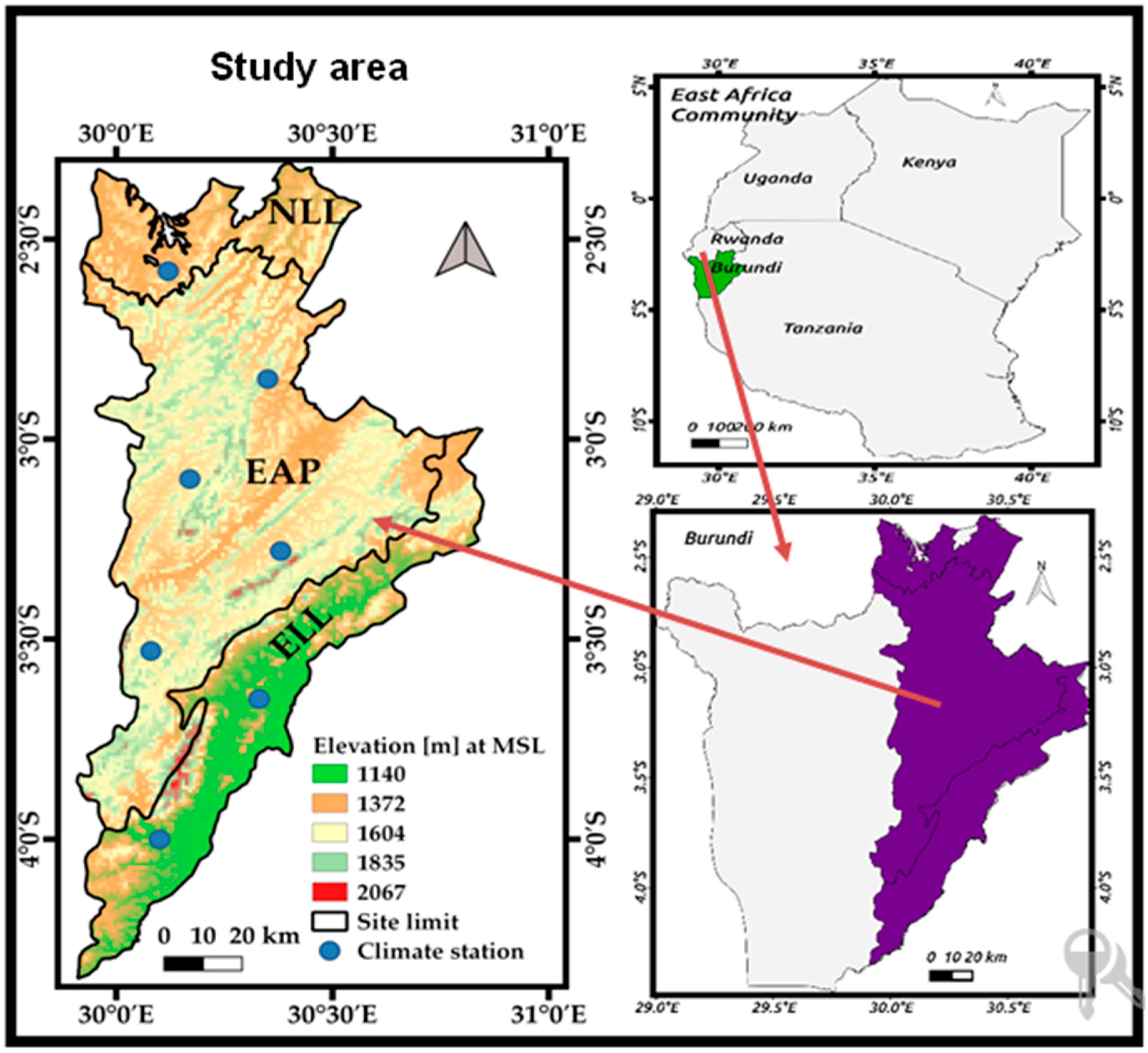However, these hydropower plants do no longer produce the amount of energy expected during the installation due to the significant decrease in the water level in the reservoir [23]. This reduction of water in the retained lakes is mainly due to the climatic changes observed in recent years, for example, the decrease in rainfall and the extension of dry season. In the East and Northeast of Burundi there are no important hydropower plants installed which can produce sufficient energy regarding the need of local population. These challenges lead to the need of developing others forms of renewable energy resources like solar energy especially in the Eastern region of Burundi. In this goal, researches conducted in this area are needed to highlight climate changes and variability of the main factors of solar energy to predict the eventual potential of solar energy production. Our study aims to investigate two climatic parameters, surface air temperature and solar irradiance over three Eastern regions of Burundi. The main objective of our research is to analyze the variability, changes and projected trends of solar irradiance, and surface air temperature to predict the eventual potential availability of solar energy in this part of the country. The study is conducted in Eastern lowlands, Northern lowlands and Eastern arid plateaus of Burundi. Specifically, the study analyzes the variability of these two parameters in the historical period and detects their trends and changes considering two future periods, namely the near future (2026–2045) and far future (2066–2085), referring to the baseline period (1986–2005).

2. Materials and Methods

2.1. Study Area

The study area is the East and Northern East of Burundi presented in Figure 1. Burundi is a small country located in East Africa between longitudes 28.8°–30.9° East and latitudes 2.3°–4.45° South [26]. Burundi is bounded in the North by the Republic of Rwanda, in the West by the Democratic Republic of Congo, and in the East and South by the Republic of Tanzania. The area of Burundi is 27,834 km² and it belongs to two major watersheds: The Nile basin with an area of 13,800 km² and Congo River basin with 14,034 km² of area [27]. The climate in Burundi, as an East African country, is mainly influenced by the North-South movement of the Intertropical Convergence Zone (ITCZ), the topography of the country and El-Nino Southern oscillation (ENSO) [23]. Then the annual mean of climate variables such as precipitation, temperature and wind speeds, depends mainly to the climate zone location. The interest study area covers the East and Northeast of Burundi and is divided into three sub-regions considering their landforms: The Eastern lowlands of Kumoso (ELL), the Eastern arid plateaus (EAP) and the Northern lowlands of Bugesera (NLL). The ELL is a region located to the extension of the border with Republic of Tanzania whereas NLL is covering two provinces (Kirundo, Muyinga) located Northeast of the country. The main different between the three regions is elevation as shown in Figure 1. This elevation defines the climate of each region and then temperature is high in lowlands regions. The annual mean temperature varies from 19 °C for EAP to 22 °C for ELL and NLL, and their altitudes also vary from 1400–2000 m for EAP to 1100–1400 m for ELL and NLL [27]. The mean yearly solar irradiance for these regions is closely the same and varies from 232 W/m²–248 W/m².

2.2. Data Used

Data of two climate parameters are considered in this study: Surface air temperature and solar irradiance as observed and projected data. The observed data used are grouped into three sets of data. The first set of data is a collection of observed data from the synoptic stations of Burundi belongs to the Geography Institute of Burundi (IGEBU). Monthly and annual mean temperature data for seven stations located in the study area are used over the historical period of thirty years (1976–2005). These climate stations are presented in Figure 1 and their geographic information and description are given in

Table 1. Geographic characteristics of meteorological stations used.

Name	B.W*	Region	Latitude South	Longitude East	Period
KIRUNDO	Nile	NLL	2.58	30.12	1976–2005
MUYINGA	Nile	EAP	2.85	30.35	1976–2005
CANKUZO	Nile	EAP	3.28	30.38	1976–2005
KARUZI	Nile	EAP	3.10	30.17	1976–2005
MURIZA	Nile	EAP	3.53	30.08	1975–2000
KINYINYA	Congo	ELL	3.65	30.33	1976–2002
MUSASA	Congo	ELL	4.00	30.10	1976–1999

B.W*: Basin watershed.

.

However, some stations had uncompleted data and shorter duration than the 30 years recommended. To complete observed data, the second set of data used is MERRA-2data set available at http://gmao.gsfc.nasa.gov/reanalysis/MERRA-2 [28] and provided by NASA/Goddard Space Flight Center.

Due to the lack of solar irradiance data measured in the stations of our study area, the third set of observed data is provided by the SoDa database available at http://www.soda-is.com [29]. Furthermore, due to the lack of long-term solar irradiance measurement, data from 1985–2005 are used as an observational solar irradiance dataset with spatial resolution of 20 km. The SoDa server provides hourly, daily, monthly and annually irradiation over Europe, Africa, and Atlantic Ocean which is accessible on free basis [30]. The SoDa irradiance is satellite-derived data of HelioClim-1 Daily solar irradiance v4.0. HelioClim-1 databases use the Heliosat-2 method to process the Meteosat images. The Heliosat-2 method converts images acquired by meteorological geostationary satellites such as Meteosat (Europe), GOES (USA) or GMS (Japan), into data and maps of solar radiation received at ground level [30].

Table 2. Data collected over the period1976–2005 for temperature and over the period1985–2005 for solar irradiance at the annual scale.

Variable	Region	Mean	Maximum	Minimum	Stdev*
tas*	NLL	20.52	21.77	19.52	0.62
	EAP	19.45	20.16	18.66	0.31
	ELL	21.74	22.37	21.03	0.60
rsds*	NLL	248.56	260.75	239.17	5.34
	EAP	236.07	248.13	225.04	5.30
	ELL	232.19	241.71	221.58	5.09

tas*: annual mean temperature in (°C), rsds*: monthly mean surface solar Irradiance in (W/m²), Stdev*: standard deviation.

describes the data collected over the period 1976–2005 for temperature and over 1985–2005 for solar irradiance at annual scale.

Climate projections data used are daily surface air temperature and solar irradiance taken from eight regional climate models available in the context of Coordinated Regional Climate Downscaling Experiment (CORDEX) over Africa at 0.44° resolution for the period 1950–2100 [31] and accessed online https://www.cordex.org [32].

Table 3. The used climatic models.

GlobalClimate Model Name	Institute ID	Model Short Name
CanESM2	CCCma	CCCma
NRM-CM5	CNRM-CERFACS	CNRM
EC-EARTH	ICHEC	ICHEC
IPSL-CM5A-MR	IPSL	IPSL
MIROC5	MIROC	MIROC
MPI-ESM-LR	MPI-M	MPI
NorESM1-M	NCC	NCC
GFDL-ESM2M	NOAA-GFDL	NOAA

presents used climatic models, home institute, and model short name adopted in this paper. Climatic models are complex programs based on atmospheric circulation including its chemistry and radiation, oceanic circulation including its biochemistry, land-surface, river routing and sea ice modeling [6]. The differences between them are mainly related to the physical parameterization of each component of the model structure. IPCC has established four Representative Concentration Pathway (RCP) scenarios which are linked to the concentration of greenhouse gas emission during the 21st century. According to the socio-economic technological and policy development activities that disturb the concentration of carbon dioxide in the atmosphere, there are RCP2.6, RCP4.5, RCP6.0 and RCP8.5 where the associated number corresponds to the radiative forcing reached at the end of 21st century [33].

In this study, experiments were performed following RCP8.5, which is the highest forcing radiative scenario, are considered for two future periods (named near future and far future) in CORDEX database. Due to the short baseline period of solar irradiance the period 2026–2045 for near future and 2066–2085 for far future have been considered for these two parameters. The RCP 8.5 is based on the A2r scenario which combines assumptions about high population and relatively low income growth with modest rates of technological change and energy intensity improvements, leading in the long term to high energy demand and greenhouse gas emissions in the absence of climate change policies [34]. This set of data is the up-to-date ensemble of high-resolution Regional Climate Model (RCM) projections, and data have been bias corrected using historical observed data.

2.3. Methods

2.3.1. Bias Correction

RCM temperature and solar irradiance were corrected for their biases in mean and standard deviation for each calendar month, following the methodology presented in Haerter et al. [35]. The bias in the mean is corrected by subtracting the differences found between observed and modeled values and a correction to the model data is performed to conform to the variability of the historical data. This procedure takes the sequence of anomalies and scales them consistently with the observed historical variability. As used by Ioanna S. Panagea et al. [30], for data following a normal distribution, the transfer function is linear and is of the form shown in the following equation:

$${\mu }_{sc}^{cor}=\left({\mu }_{mod}^{sc}-\overline{{\mu }_{mod}^{con}}\right)\ast \left(\frac{{\sigma }_{obs}^{con}}{{\sigma }_{mod}^{con}}\right)+\overline{{\mu }_{obs}^{con}}$$

(1)

where ${\mu }_{sc}^{cor}$ is the final adjusted time series, ${\mu }_{mod}^{sc}$ is the raw model predictions for the scenario period $\overline{{\mu }_{obs}^{con}}$ and $\overline{{\mu }_{mod}^{con}}$ are the mean of observed and modeled data for the control period, respectively, and ${\sigma }_{obs}^{con}$ and ${\sigma }_{mod}^{con}$ are the standard deviations of observed and modeled data for the control period, respectively. The final adjusted model time series exhibits the appropriate baseline mean and standard deviation with respect to the observed data [30].

2.3.2. Variability Analysis

The discrimination of high or low values of each climate parameter considered was done by computing the standardized variable index (I) created by Reference [36] and which can be found in many articles [37,38]. Then, the standardized variable index (I) is defined by Equation (2):

$$I\left(i\right)=\frac{{\chi }_i-{\overline{\chi }}_m}{\sigma },$$

(2)

where ${\chi }_i$, ${\overline{\chi }}_m$ and $\sigma$ are respectively the value for the considered year (or month $i$), the average and the standard deviation of the time series. Thus, in this work we considered that a year is normal when its index is included between −0.5 and +0.5. It will be in surplus if its index is greater than +0.5, and will be considered as deficit when its index is below than −0.5. This interval is relatively weak and is criticized but it allows distinguishing of the deficit years from surplus years. The standardized variable index makes also possible to analyze the interannual variability of the variables at considered time scale.

2.3.3. Future Climate Analysis

The temporal assessment of the future climate has been done using Regional climate models (RCM) over two periods named near future and far future. The period 2026–2045 and 2066–2085 for surface air temperature and surface solar irradiance have been considered with respect of the reference period 1986–2005. Following RCP8.5 scenario, eight RCM (CCCma, CNRM, ICHEC, IPSL, MIROC, MPI-M, NCC and NOAA) are used to plot projected trends at annual scale and a linear trend has been plotted to show the multi model’s trend, after bias correction according to observational data set. Furthermore, a multi-model mean has been computed and adopted at a monthly scale.

The analysis of climate changes was done in two steps according to two future periods considered in this study with reference to the baseline period. We compute and add delta change factors to monthly time series of observation records. The calculations of delta change factors were based on a selected projection interval (2026−2045) with a baseline period (1986–2005) for both temperature and solar irradiance using the Equations (3). The same computation was repeated with the selected projection interval (2066−2085). Then the change factors for temperature and solar irradiance were determined by:

$$\Delta {\mu }_{i,j,k}={\overline{\mu }}_{i,j,k}-{\overline{\mu }}_{ref,k}$$

(3)

where $\Delta \mu$ is the change factor (°Cor w/m²), $\overline{\mu }$ is the monthly mean (°Cor w/m²), i is the RCM, j is the projection period, ref is the reference period and k is the month.

Two statistics tests, Mann Kendall and t-test have been used respectively to clarify the trends detected of a time series and to test the mean equality of two times series for each variable. The Mann Kendall’s test (MK) [39,40], which is used by many authors, was used for detecting trends in time series. MK checks increasing, decreasing, or no trends of the projected models mean time series of the three regions of our study area. If there is a linear trend in the time series, the true slope has been estimated using Sen’s slope method [21] which is a simple non- parametric found in many articles [41,42]. Furthermore, the t-test [43] has been used to prove whether the difference between two ensemble models means over the baseline and future period is statistically significant for a considered region. Before using the t-test, which is a parametric test, normal distribution of the used data must be assessed.

3. Results and Discussions

3.1. Variability Analysis in the Historical Period

3.1.1. Seasonal Temperature

Figure 2 presents the monthly temperature patterns at NLL, EAP and ELL over the historical period 1976–2005 and monthly standardized temperature index for the same period.

The analysis of Figure 2a shows that June and July present low mean values of temperature, whereas September and October show high mean values but the pattern does not show remarkable variations. This figure reveals also that ELL has high values and EAP has low values of surface air temperature over the year.

The means monthly temperature for NLL, EAP and ELL used to calculate the standardized variable index are respectively 20.56 °C, 19.38 °C and 21.75 °C. In the same way, the standard deviations are 0.54, 0.61, and 0.92 respectively for NLL, EAP and ELL. The analysis of Figure 2b shows that six months (April, May, June, July, November and December) are cooler at NLL while three months (May, June and July) are cooler at EAP and ELL. The coolest month with the lowest index value equal to −1.66 is July for ELL while the coolest month is June for NLL and EAP with the lowest index values equal to −1.27 and −1.51, respectively. The analysis shows also that four months (February, August, September and October) are hotter at NLL, while three months (August, September and October) are the warmest at EAP and only two months are the hottest (September and October) at ELL. Normal months in the year are January, February, March, November and December for all regions except NLL where normal months are January and March only. The hottest month is September for both regions with the highest index values equal to 1.87, 1.89, and 1.74 respectively for NLL, EAP, and ELL.

3.1.2. Interannual Temperature

Figure 3a presents the interannual temperature patterns for the period 1976–2005 at NLL, EAP and ELL. This figure shows that the ELL is the hottest region with about mean value of 21.7 °C whereas EAP is the coolest region of the study area with the 19.4 °C of annual mean value. This high temperature over low land is due to the low altitude and as we can remark that there is an upward trend with the increase changes.

Figure 3b shows interannual standardized temperature at NLL, EAP, and ELL over the period 1976–2005. The analysis of this figure points out two sub-periods, including the first period 1976–1991 with more cool years, except 1980, which has high values of mean temperature for the three regions, and 1983, which has a high value of average temperature for NLL only. The second sub-period includes the period 1992–2005 with more hot years except 1996 and 1997 which have low mean temperature for all regions and 2001 which is the coolest year for EAP only. The analysis of the figure shows also 11 years of high temperature for NLL and EAP and 9 years of high temperature for ELL while 10 years of low temperature are observed at NLL and, 9 years of low temperature at EAP and ELL.

These results reveal an upward trend of average temperature for the last sub-period1992–2005 and pointed out the hottest years occurred in 1999 for NLL and ELL and 1998 for EAP whereas the coolest years occurred in 1986 for EAP and ELL with 1978 for NLL. Furthermore, these findings agree with the results of many studies which show increases in temperature over the end of the last century, See References [19,22,44]. More recently, the study of Birara et al. [21] analyzed the trend and variability of Rainfall and temperature in the Tana basin region, Ethiopia, for the period covers 1980–2015 and found the significant increases of maximum, minimum and mean temperature for most of the stations considered and an increase of 1.08 °C was observed. These increases in temperature may affect negatively the production of solar energy and increase evaporation which reduces water availability.

3.1.3. Seasonal Solar Irradiance

Figure 4 presents the monthly solar irradiance patterns and standardized solar irradiance at NLL, EAP and ELL over the period 1985–2005. The analysis of Figure 4a shows a bimodal seasonal cycle with peaks respectively reached at February and July. The month December presents the lowest mean value of solar irradiance for all regions whereas the month July displays the highest mean value of solar irradiance for all regions. Figure 4a reveals also that NLL has high values and ELL has the low values of mean solar irradiance over the year but for month June, July and August, there are mixture values of EAP and values of ELL.

Figure 4b presents the monthly standardized solar irradiance at NLL, EAP and ELL over the historical period. The analysis of this figure shows that four months (April, May, November and December) are in deficit of solar irradiance at NLL and four months also (January, May, November and December) are in deficit of solar irradiance at EAP and ELL. The month with the lowest index value equal to −1.4 is May for NLL while the month with low value of solar irradiance is December for ELL and EAP with the lowest index value equal to −1.26 and −1.13, respectively. The analysis shows also that four months (February, July, August and September) are in excess of solar irradiance at NLL while four months also (June, July, August and September) for ELL with three months (July, August, September) at EAP are in excess of solar irradiance. Normal months are February, March, April and October for EAP and ELL whereas January, March, June and October are normal for the region of NLL. The Month with highest index value of solar irradiance is July for all regions with 1.89, 1.95, and 1.65 for NLL, EAP and ELL, respectively.

The monthly means solar irradiance for NLL, EAP and ELL used to calculate the standardized variable index are respectively 248 W/m², 236 W/m², and 231 W/m², whereas standard deviationsare 10.9, 13.2, and 19.5 respectively for NLL, EAP, and ELL. This analysis shows that the months with highest values of solar irradiance coincide with the dry season, which leads to the conclusion that there is an excess of solar irradiance in the dry season and, therefore, it must be a period of high production of solar energy. Indeed, a solar power plant installed in this region could be in complementary with a hydroelectric plant with low production in the dry season because of the reduction of the water level in the reservoir.

3.1.4. Interannual Solar Irradiance

The Figure 5a gives the interannual solar irradiance patterns for the period 1985–2005 at NLL, EAP and ELL. This figure shows that NLL indicates high values of solar irradiance than other regions which have close values over the full period. In the other hand, this pattern does not show long variability of solar irradiance values through the historical period. We can also observe that EAP and ELL have likely the same values and there are not many differences, and some months show a mixture of solar irradiance values.

Figure 5b presents interannual standardized solar irradiance at NLL, EAP, and ELL over the historical period 1985–2005. The analysis of this figure points out three sub-periods including the first period spanning from 1985–1988 with high values of solar irradiance and some years with normal values but no year with low values of solar irradiance for all three regions of the study area. The second sub-period 1989–1998 presents mixture years with high, low and normal values of solar irradiance for all regions. The third sub-period 1999–2005 is marked by many years with low values of solar irradiance and a few normal years, but there is no year with high values of solar irradiance observed for the three regions of the study area. The analysis of the features shows also 6 years with high values of solar irradiance for NLL, EAP, and ELL, while 7 years with low values of solar irradiance are observed at NLL and ELL, and 6 years have low values of solar irradiance at EAP. These results reveal a downward average solar irradiance trend for the last sub-period 1999–2005 and pointed out the year with lowest values occurred in 2001 for all three regions whereas the year with highest values of solar irradiance occurred in 1987 for EAP, ELL, and NLL.

This analysis shows also a general upward of average solar irradiance for the first sub-period. Furthermore, these findings agree with the results of many studies which revealed a subsequent increase (1–4 W/m²) since the 1980s called “brightening” [9] and decreasing of irradiation in some regions of the world. Solar irradiation is the principal resource of solar power output (PV); these decreases of this parameter affect negatively the production of solar energy.

3.2. Future Climate Analysis

3.2.1. Monthly Scale Changes

Temperature

Figure 6a presents the projected monthly surface air temperature over the period 2026–2045 and 2066–2085 according to reference period 1986–2005. The data used for future projected temperature are the mean values of eight RCMs after bias correction and the reference period were presented by observed data from stations and mean values of raw RCMs. For the near future, the analysis of Figure 6a projects an increase in surface air temperature from January to September but also projects a small decrease from October to December for all regions according to the reference period. The highest increase is projected to be in July which reaches the maximum of 3.88 °C at ELL. On the other hand, the highest decrease is projected in November and reaches the minimum of −0.93 °C at ELL also. The hottest month is projected to be September for NLL and ELL, except for EAP, which is projected to be August, and the highest value will reach 24.79 °C at ELL. Then, the coolest month is forecasted to be November for all regions, with the lowest value of 18.84 °C at EAP.

The far future period 2066–2085 projects greatest increases of surface air temperature compared to the near future as observed in Figure 6a. The highest increase is projected to be in July also with a maximum change value of 4.85 °C and the lowest increase is forecasted to be in November with a change value of 0.06 °C. For this period, the hottest month is projected to be September for all regions where the highest value is projected to be 26.00 °C at ELL. Otherwise the coolest month is forecasted to be November for all regions and lowest value is forecasted to be 19.54 °C at EAP. The findings of this study are closely in accordance with many studies carried out before locally or at regional scale. Reference [23] assessed the trends and changes detection in rainfall, temperature and wind speed in Burundi using seven RCMs up the period 2021–2050 and found that all models predict increases in temperature and wind speeds compared to the baseline period, 1981–2010.

Solar Irradiance

Figure 6b indicates the projected monthly solar irradiance over the period 2026–2045 and 2066–2085 according to the baseline period 1986–2005 at NLL, EAP, and ELL. The data used for future projected solar irradiance are the mean values of eight RCMs used after bias correction, whereas observed data from Soda and raw CORDEX data are used to present the historical period. For the first period (2026–2045), the analysis of this figure distinguishes two parts of the pattern. The first one shows an increase in solar irradiance from January to June with the maximum change occurred in March for all regions. The highest percentage changes values are 7.97%, 8.76%, and 13.53%, respectively, at NLL, EAP, and ELL. The second part shows a decrease in solar irradiance from July to December with a maximum change occurred in July for NLL and EAP, and November for ELL. The lowest percentage changes values are −7.96% and −7.71% at NLL and EAP respectively and −13.85% at ELL. Moreover, the highest value of solar irradiance is projected to be in February for all regions with 270.63 w/m², 258.27 w/m² and 262.97 w/m² at NLL, EAP and ELL, respectively. The lowest value of solar irradiance is projected to be in November with 221.37 w/m², 203.58 w/m² and 183.45 w/m² at NLL, EAP and ELL, respectively. We can note that the highest monthly changes (increases or decreases) in solar irradiance are observed in ELL.

In the same way, for the far future period the figure gives the projected monthly solar irradiance over the period 2066–2085 according to the baseline period 1986–2005 at NLL, EAP, and ELL. The analysis of this figure also shows a mixture of increasing and decreasing over the pattern: The increases in solar irradiance occurred from January to June and September, with the maximum change found in March for all regions.

The highest percentage changes values are 8.27%, 9.53%, and 15.03% respectively at NLL, EAP and ELL. The decreases in solar irradiance appeared in July and August and from October to December with a maximum decrease change occurred in November for NLL, EAP, and ELL. The highest percentages of decreasing changes are −12.05%, −12.25%, and −17.29% at NLL, EAP and at ELL respectively. Moreover, the highest value of solar irradiance is projected to be in March for all regions with 264.8 w/m², 254.1 w/m² and 258.4 w/m² at NLL, EAP, and ELL respectively. The lowest value of solar irradiance is projected to be in November with 211.5 w/m², 194.75w/m² and 176.15 w/m² at NLL, EAP, and ELL respectively.

3.2.2. Interannual Trends and Changes

Temperature

The spatial distribution of observed, models raw mean values of temperature for the reference period and projected RCMs annual mean values of temperature after bias correction over the period 2026–2045 and 2066–2085 is given by Figure 7 following rcp 8.5 scenario. The annual mean temperature is expected to increase in the future all over the regions studied. The analysis of this figure shows that this increasing change is very marked in the far future rather than the near future. Furthermore, the region ELL which is experiencing high temperature is expected to have higher increase changes than other regions, whereas the low increase changes are expected at EAP for both future periods. The projected increase in temperature found in this paper is consistent with the findings by Brohan et al. [19] and may be attributed to global warming. These features will affect the lifestyle of the population in these regions and may present a negative effect on solar energy production because an increase of temperature affects negatively the PV power output.

For projected changes in interannual average temperature,

Table 4. Changes in annual temperature (2026–2045).

	1986–2005			2026–2045
Model	Average Annual tas*(°C)			Average Annual tas*(°C)			Change (°C)
	EAP	ELL	NLL	EAP	ELL	NLL	EAP	ELL	NLL
CCCma	22.0	22.1	22.0	21.3	25.6	23.6	−0.7	3.5	1.6
CNRM	19.6	20.0	19.7	20.5	23.6	22.6	0.8	3.7	2.9
ICHEC	19.0	19.3	19.0	21.0	24.6	23.7	2.0	5.2	4.8
IPSL	21.6	21.8	21.8	20.8	24.3	23.2	−0.8	2.5	1.5
MIROC	20.1	20.4	20.2	20.5	23.9	22.4	0.4	3.4	2.2
MPI	20.0	20.3	20.1	20.7	24.1	23.0	0.7	3.8	2.9
NCC	20.5	20.7	20.7	20.6	24.0	22.7	0.1	3.3	2.0
NOAA	19.8	20.1	19.8	20.5	23.8	22.4	0.6	3.7	2.6
Mo-mean*	20.3	20.6	20.4	20.7	24.2	23.0	0.4	3.6	2.6
Observed	19.4	21.7	20.5	-	-	-	-	-	-

tas*: annual mean temperature in (°C), Mo-mean*: ensemble models mean.

and

Table 5. Changes in annual temperature (2066–2085).

	1986–2005			2066–2085
Model	Average Annual tas*(°C)			Average Annual tas*(°C)			Change (°C)
	EAP	ELL	NLL	EAP	ELL	NLL	EAP	ELL	NLL
CCCma	22.0	22.1	22.0	23.2	29.5	26.8	1.2	7.3	4.8
CNRM	19.6	20.0	19.7	22.2	26.8	25.9	2.5	6.9	6.2
ICHEC	19.0	19.3	19.0	23.3	28.8	28.3	4.3	9.4	9.3
IPSL	21.6	21.8	21.8	22.9	28.4	27.5	1.3	6.6	5.7
MIROC	20.1	20.4	20.2	21.7	26.3	24.6	1.6	5.8	4.4
MPI	20.0	20.3	20.1	22.7	27.4	26.8	2.7	7.2	6.7
NCC	20.5	20.7	20.7	22.3	27.0	26.1	1.8	6.3	5.4
NOAA	19.8	20.1	19.8	21.3	25.4	24.1	1.5	5.3	4.3
Mo-mean	20.3	20.6	20.4	22.4	27.5	26.3	2.1	6.9	5.9
Observed	19.4	21.7	20.5	-	-	-	-	-	-

tas*: annual mean temperature in (°C), Mo-mean*: ensemble models mean.

show changes in projected average temperature at annual scale for the two periods considered. Used data are each model raw mean value for the reference period and projected RCMs annual mean values of temperature. The analysis of the Table 4 shows that at EAP, ELL, and NLL will experience a change of 0.4 °C, 3.6 °C, and 2.5 °C by 2045 in the ensemble models-mean according to the baseline period 1986–2005. In the same way, the analysis of the Table 5 shows that a change of 2.1 °C and 6.9 °C and 5.9 °C are respectively expected in the ensemble models mean at EAP, ELL and NLL by 2085 according to the reference period 1986–2005.The analysis of the two tables shows that higher changes are normally expected in the far future rather than the near future. We can note that there are few decrease changes in the near future, especially at EAP region predicted by CCCma and IPSL. Indeed, the highest changes occurred at ELL and are predicted by ICHEC in both future periods. In general, ELL presents high deltas for almost all models over all regions and for ensemble models mean. Therefore, the lowest change occurred at EAP with IPSL in the near future and with CCCma by 2085.Furthermore, with a significant level of 0.05, the ensemble models mean differences between the baseline period and each of two future periods are statistically significant over all regions according to the t-test with a p-value less than 0.0001. However, an ensemble models mean difference between 1986–2005 and 2026–2045 at EAP presents a slight significance compared to others regions, as well as observed value |t| is very close to critical value. Given that t-test is a parametric test, a normal distribution of all temperature data used has been controlled.

For trend detection in projected average temperature at significance level α = 0.05, the Mann Kendall’s test(MK) revealed upward trends all over the regions for both periods 2026–2045 and 2066–2085 with a very small p-value = 0.0001. Indeed, the Kendall’s tau for both periods is likely the same. In fact, over the period 2026–2045 the Kendall’s tau equals to 0.81 for EAP, 0.75 for ELL and it equals 0.82 for NLL, while in period 2066–2085 the Kendall’s tau is 0.77 for EAP and 0.80 for ELL and NLL. Combined with the Sen’s slope method, these statistical tests revealed upward trends of surface air temperature in the considered periods all over the regions of the study area.

Solar Irradiance

Figure 8 presents a spatial distribution of annual mean of solar irradiance data from Soda database (observed), annual mean from original CORDEX in the reference period 1986–2005 and projected models mean of solar irradiance after bias correction over two future periods namely near future 2026–2045 and far future 2066–2085. Following rcp 8.5, the entire region does not show the highest change either in the near future or far future. However, the analysis of the figures shows that NLL is experiencing high values of solar irradiance whereas ELL presents low values. In addition, a slight downward trend of solar irradiation is also observed generally in far future over all regions. Furthermore, the analysis of this figure shows also that the highest changes are observed at EAP for both future periods.

The projected changes in solar irradiance for the period 2026–2045 are summarized in

Table 6. Changes in annual solar irradiance (2026–2045).

	1986–2005			2026–2045			Change (w/m2)			Change (%)
Model	Average Annual rsds* (w/m2)			Average Annual rsds* (w/m2)
	EAP	ELL	NLL	EAP	ELL	NLL	EAP	ELL	NLL	EAP	ELL	NLL
CCCma	240.6	237.4	251.6	235.5	231.8	247.1	−5.0	−5.6	−4.5	−2.1	−2.4	−1.8
CNRM	263.6	257.1	274.0	234.6	231.7	246.1	−29.0	−25.4	−27.9	−11.0	−9.9	−10.2
ICHEC	243.3	236.5	255.5	233.5	230.4	244.9	−9.8	−6.2	−10.7	−4.0	−2.6	−4.2
IPSL	243.5	239.1	253.7	229.0	227.6	241.8	−14.6	−11.5	−11.8	−6.0	−4.8	−4.7
MIROC	252.5	246.7	262.1	234.3	230.9	245.5	−18.2	−15.8	−16.6	−7.2	−6.4	−6.3
MPI	251.4	245.7	262.1	234.0	230.9	245.7	−17.4	−14.8	−16.4	−6.9	−6.0	−6.3
NCC	253.9	248.0	264.2	230.4	228.0	240.6	−23.6	−20.0	−23.6	−9.3	−8.1	−8.9
NOAA	245.5	238.9	258.6	237.2	233.6	248.7	−8.3	−5.3	−10.0	−3.4	−2.2	−3.9
Mo-mean*	249.3	243.7	260.2	233.6	230.6	245.0	−15.7	−13.1	−15.2	−6.3	−5.4	−5.8
Observed	236.1	232.2	248.6	-	-	-	-	-	-	-	-

Mo-mean*: ensemble models mean, rsds*: surface solar irradiance.

, while

Table 7. Changes in inter annual solar irradiance (2066–2085).

	1986–2005			2066–2085			Change (w/m2)			Change (%)
Model	Average Annual rsds (w/m2)			Average Annual rsds (w/m2)
	EAP	ELL	NLL	EAP	ELL	NLL	EAP	ELL	NLL	EAP	ELL	NLL
CCCma	240.6	237.4	251.6	231.7	228.5	242.2	−8.9	−9.0	−9.4	−3.7	−3.8	−3.7
CNRM	263.6	257.1	274.0	234.8	232.9	245.3	−28.8	−24.3	−28.7	−10.9	−9.4	−10.5
ICHEC	243.3	236.5	255.5	232.4	231.1	241.3	−11.0	−5.5	−14.2	−4.5	−2.3	−5.6
IPSL	243.5	239.1	253.7	218.0	217.3	228.2	−25.5	−21.7	−25.4	−10.5	−9.1	−10.0
MIROC	252.5	246.7	262.1	233.3	230.3	243.1	−19.3	−16.4	−19.0	−7.6	−6.6	−7.3
MPI	251.4	245.7	262.1	232.2	230.7	241.2	−19.2	−15.0	−20.8	−7.6	−6.1	−8.0
NCC	253.9	248.0	264.2	230.6	229.3	240.9	−23.3	−18.7	−23.3	−9.2	−7.5	−8.8
NOAA	245.5	238.9	258.6	235.2	232.5	245.5	−10.3	−6.4	−13.1	−4.2	−2.7	−5.1
Mo-mean*	249.3	243.7	260.2	231.0	229.1	241.0	−18.3	−14.6	−19.3	−7.3	−6.0	−7.4
Observed	236.1	232.2	248.6	-	-	-	-	-	-	-	-	-

Mo-mean*: ensemble models mean, rsds*: surface solar irradiance.

presents the projected changes for far future 2066–2085 both using each raw model mean value over the reference period and projected RCMs annual mean values of solar irradiance. The two tables show that the projections are very close; therefore, the last table presents a higher decrease of solar irradiance in far future than near future.

The analysis of Table 6 shows that the multi models mean project a decrease change of −6.3%, −5.4%, and −5.8% at EAP, ELL, and NLL, respectively. Indeed, the highest decreasing change is projected by NCC at EAP.

Compared with the findings shown in Table 7, these results predict low decrease of solar irradiance than far future as said before. In fact, the results obtained in period 2066–2085 presented in the Table 7 show projected changes of −7.6%, −6.0%, and −7.4% by the ensemble models mean at EAP, ELL, and NLL. Indeed, the highest change is forecasted by CNRM at EAP and the value is −10.9%. Even if NLL presents high values of solar irradiance, ELL and NLL are expected to have high deltas changes for almost all models and for ensemble models mean. The analysis of these two tables reveals that surface solar irradiance will experience small annual changes in the future which determine an interest of installing solar power plan in the regions. Despite the slight decreasing of solar irradiance predicted over all regions, the ensemble models mean differences between baseline and near future or far future are significant over all regions regarding t-test’s results with a significant level α = 0.05. In fact, the p-value is very lower than α and the observed value |t| is greater than the critical value. Before using the parametric t-test, a normal distribution of solar irradiance data is evaluated for all periods and over all regions.

For trend detection over the period 2026–2045, the MK’s test indicates no significant trend in forecasted surface solar irradiance at significance level α = 0.05 following rcp 8.5 scenario for all the regions. The same conclusion is observed over the far future for all the regions. In fact, the p-values found of all time series are greater than α = 0.05 for the far future and near future, so the null hypothesis which assumes a trend can be rejected. Therefore, the Sen’s slope showed a downward trend in the ensemble model mean with small values of −0.012, −0.03 and −0.114 respectively at EAP, ELL and NLL over the near future period. In the same way, a downward trend is also detected by the Sen’s slope with small values of −0.089, −0.077 and −0.167 respectively at EAP, ELL, and NLL over far future. Even if the MK’s test is not significant, the trends of solar irradiance predict a small decreasing feature for a long time.

4. Conclusions

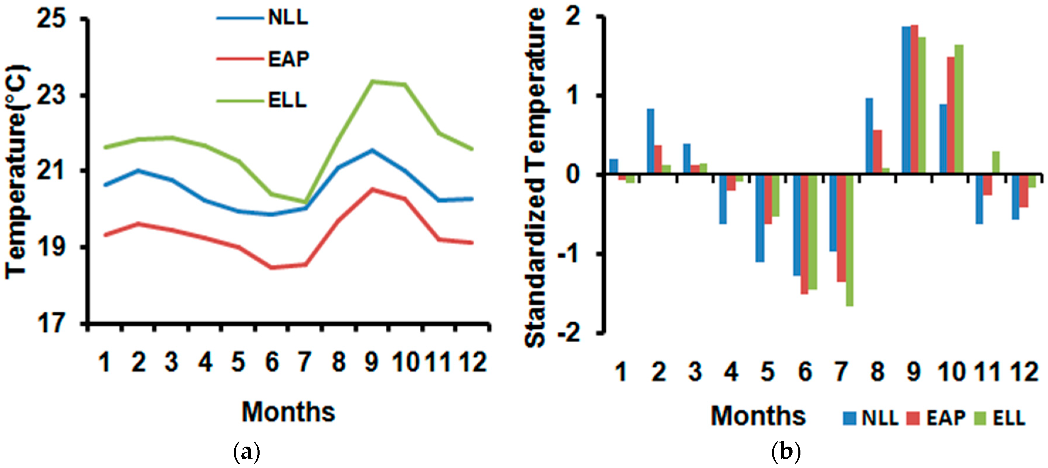
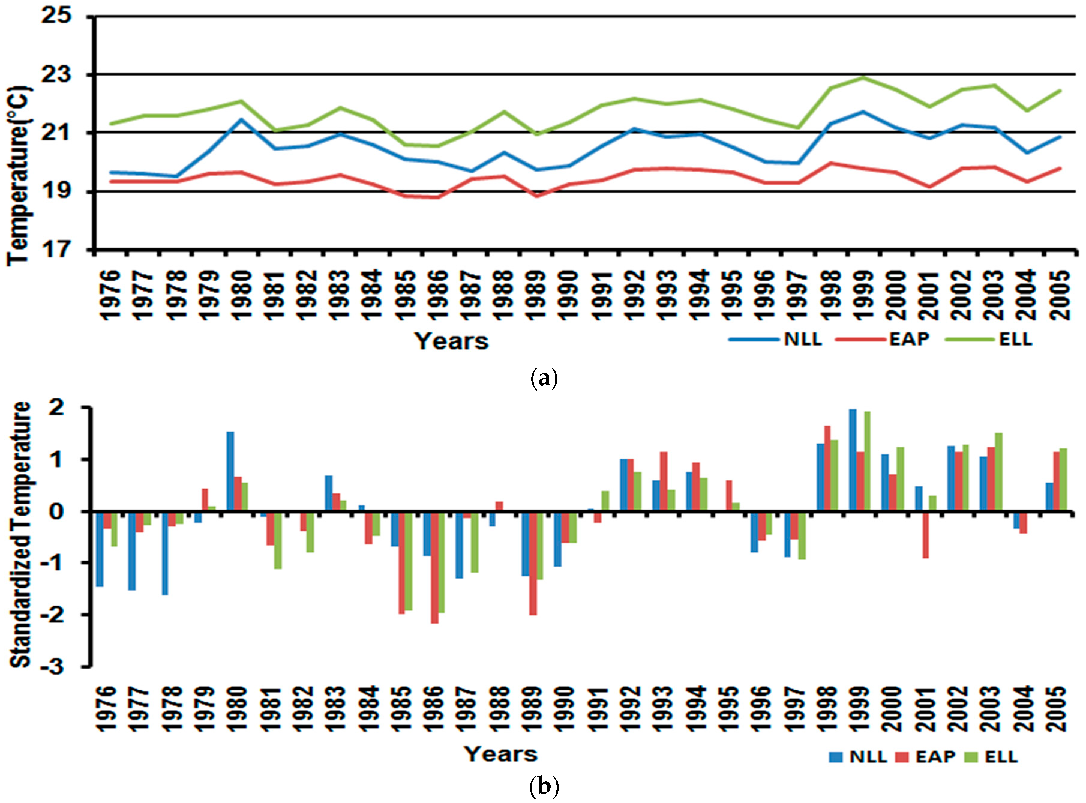
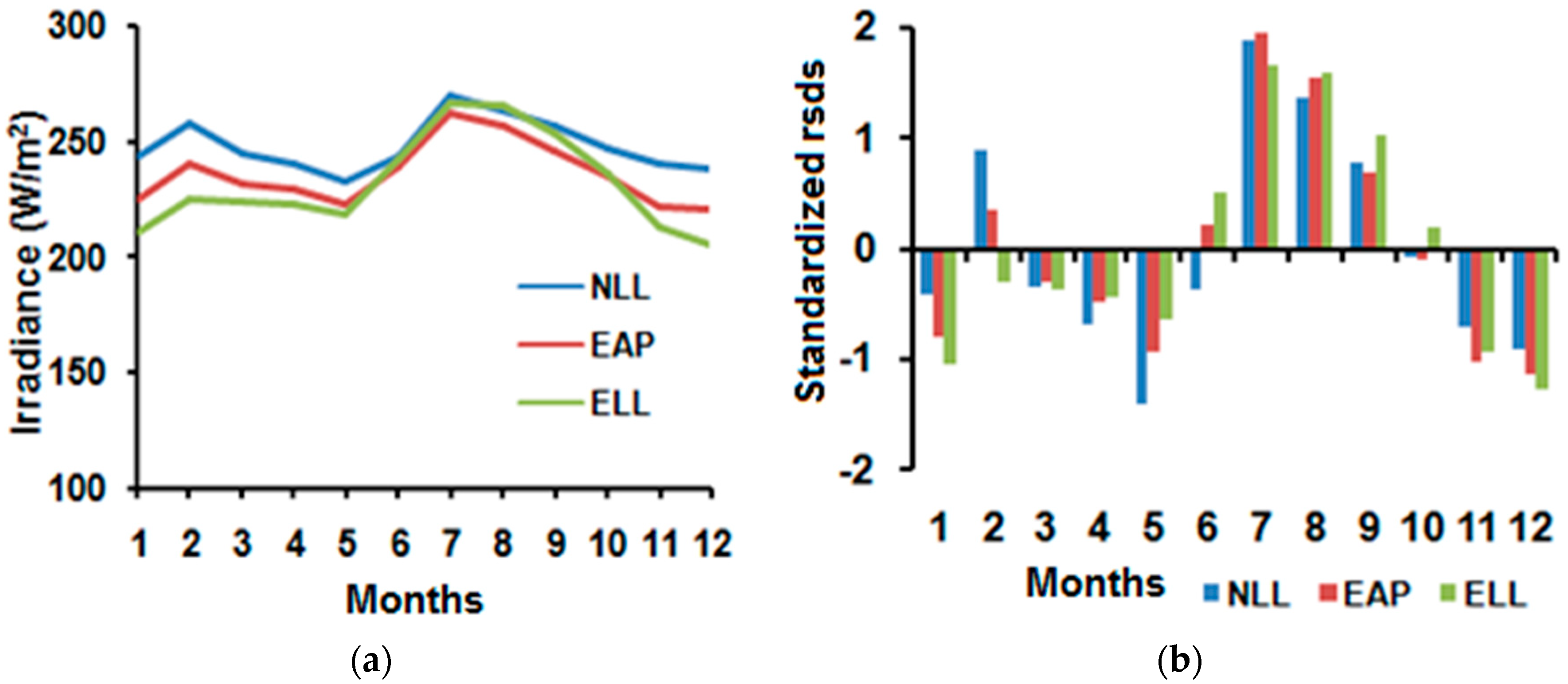
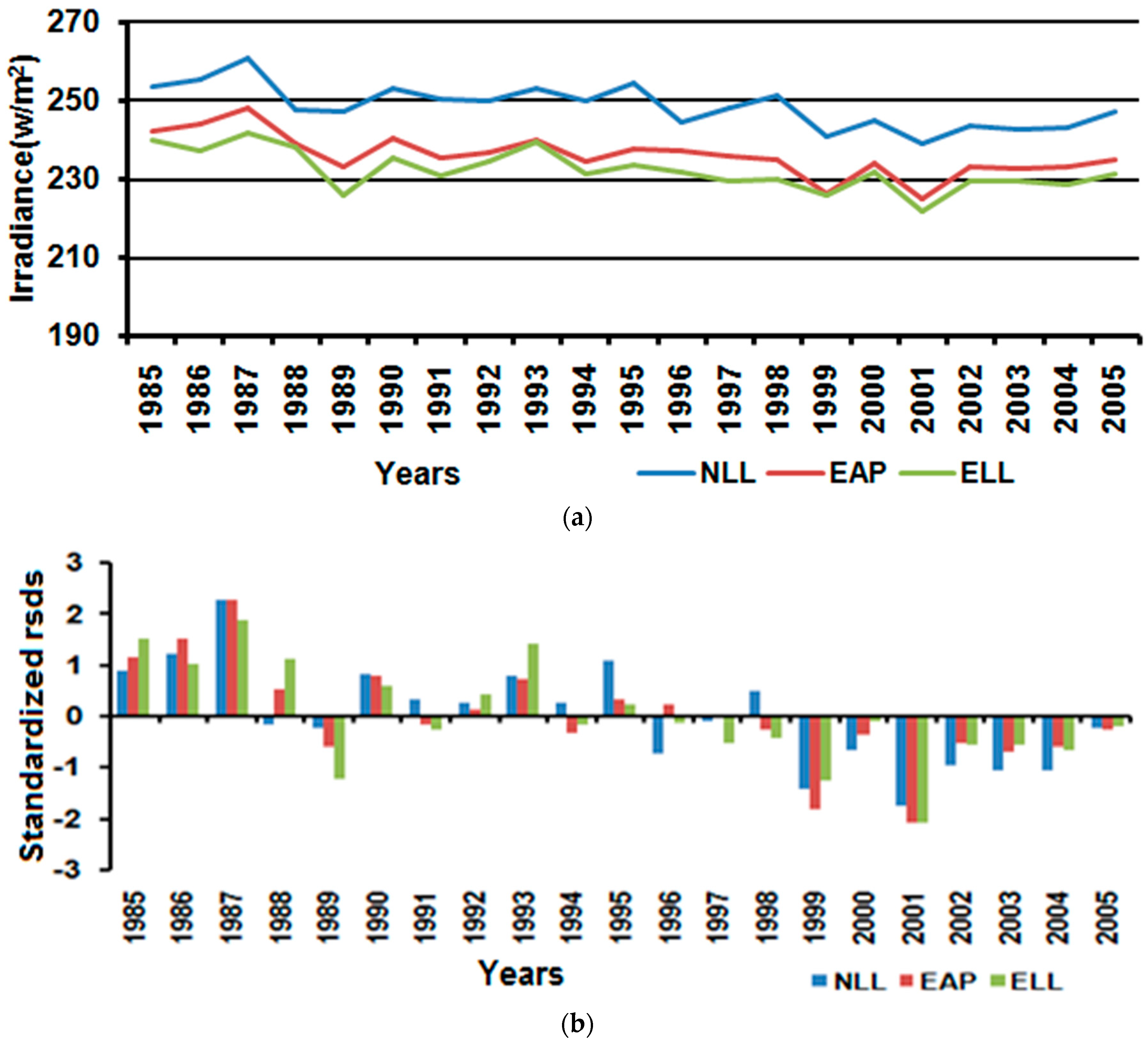
The analysis of variability and projected trends of temperature and solar irradiance has been performed considering historical period and two future periods. Observed temperature data from meteorological stations and solar irradiance data from the Soda database were used over the historical period. In addition, projection data from eight Regional Climate Models were used over the periods 2026–2045 and 2066–2085 after bias correction for their mean and standard deviation in order to produce correctly the future climate and conform to the observed data. The characterization of the historical period was done using the standardized variable index for each climatic parameter. The interannual results revealed an upward trend in average temperature for the last sub-period 1992–2005. At the monthly scale, the analysis showed seasonal variability where an upward trend in average temperature appears from August–October, and the hottest month is September for all regions. A downward trend occurred from May–July, and the coolest month is July. For solar irradiance, the monthly analysis showed that the surplus months coincide with the dry season, which leads to the conclusion that there is an excess of solar irradiance in the dry season with the highest value appearing in July. The interannual results revealed a downward trend in average solar irradiance for the last sub-period 1999–2005 and showed also a general upward trend in average solar irradiance for the first sub-period.

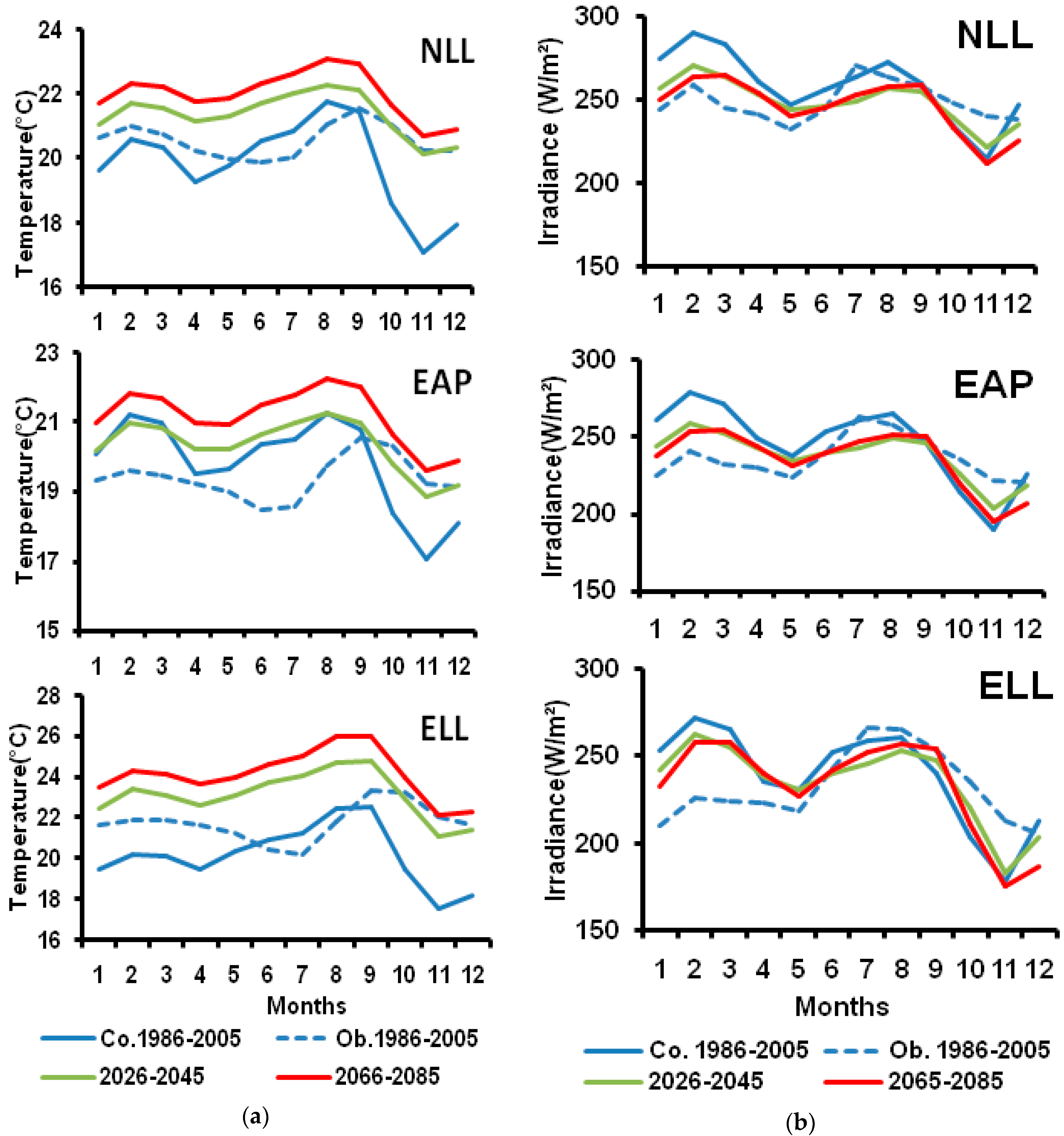
For future analysis, at a monthly level, an increase in surface air temperature from January–September and a small decrease from October–December are projected for all regions according to the reference period. Therefore, the far future presents the same features as the near future with a high amplitude of increase over the far future. The highest increase is projected to reach a maximum change value of 4.85 °C. The hottest month is projected to be September for all regions where the highest value is projected to be 26.00 °C at ELL. For solar irradiance, the seasonal analysis distinguishes two parts of the pattern for both periods. The first one shows an increase in solar irradiance from January–June with the maximum change occurring in March for all regions. The second part shows a decrease in solar irradiance from July–December with a maximum change occurring in July for NLL and EAP, and November for ELL. The analysis of the results revealed that the far future presents the same features as the near future, where the changes are very marked over the far future.

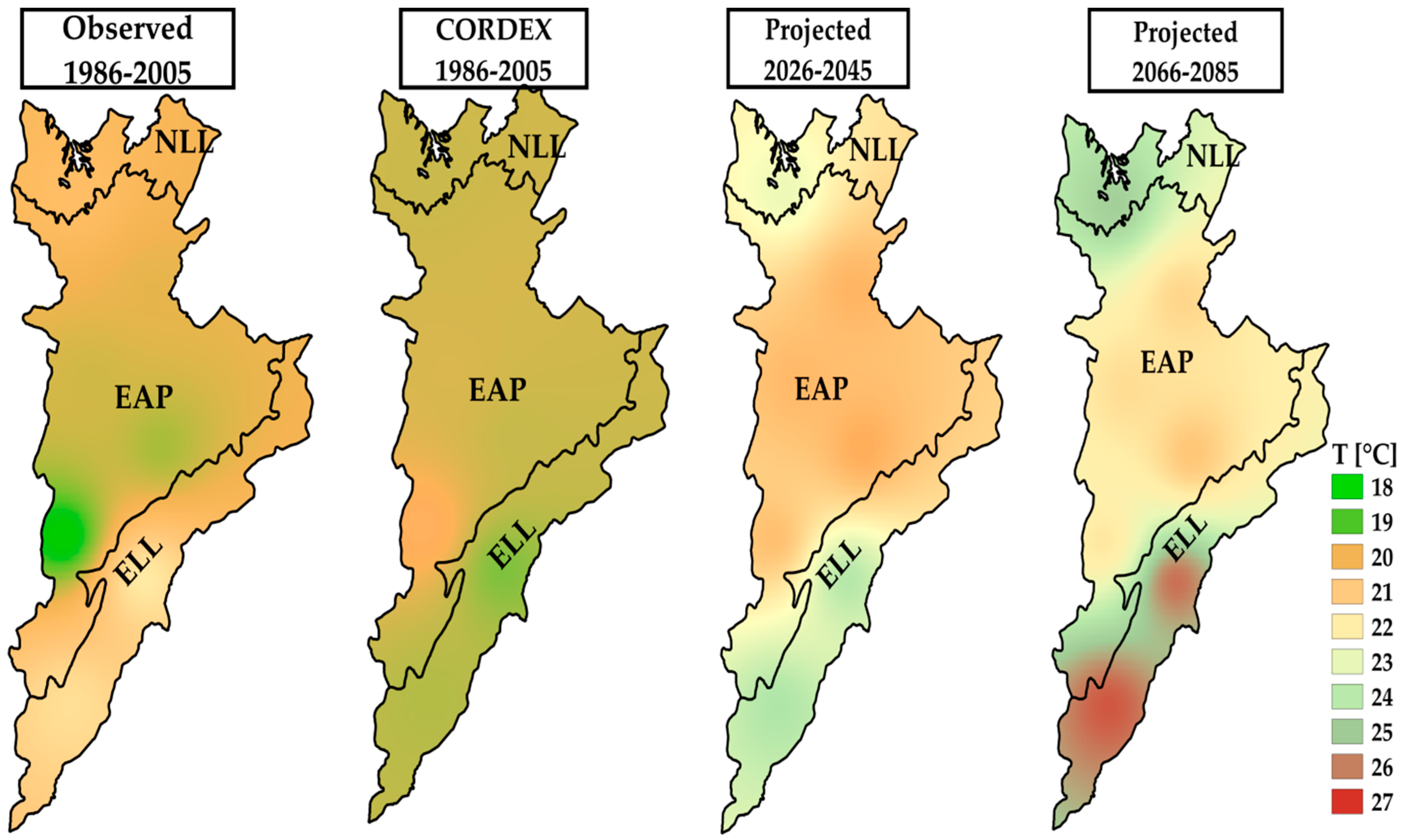
At the interannual scale, considering air ambient temperature, the results show that lowlands are expected to be hotter than arid plateaus. For trend detection in projected average temperature at significance level α = 0.05, the MK’s test revealed upward trends all over the regions for both the future periods. The ensemble models mean differences between the baseline period and each of the two future periods are statistically significant over all regions according to t-test. Considering projected changes, the analysis shows that at EAP, ELL, and NLL will experience a change of 0.4 °C, 3.6 °C, and 2.6 °C by 2045 in the ensemble models mean according to the baseline period 1986–2005, whereas changes of 2.1 °C and 6.9 °C and 5.9 °C are respectively expected in the ensemble models mean at EAP, ELL, and NLL by 2085. The analyses show also that higher changes are normally expected in the far future than the near future.

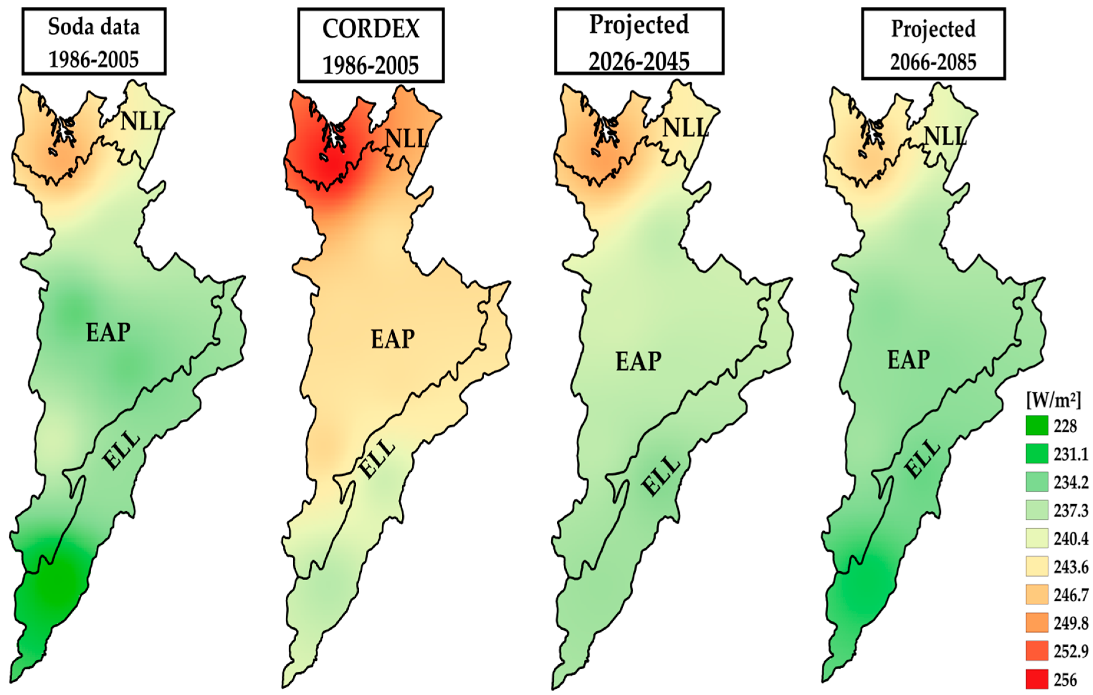
Interannual analysis of solar irradiance shows clearly a slight downward trend of solar irradiance for both periods. The results predict a downward average of solar irradiance over all regions studied and for all models used. For trend detection over both periods, the MK’s test indicates no significant trend in forecasted solar irradiance at a significance level α = 0.05 over allregions. Therefore, the Sen’s slope showed a downward trend in the ensemble models mean with small values over the near future and far future periods. The ensemble models mean differences between baseline and near future or far future are significant over all regions regarding t-test’s results. The projected changes in solar irradiance show that the projections are very close over two periods. The multi models mean projected the decreasing changes of −6.3%, 5.4%, and 5.8% at EAP, ELL and NLL respectively over 2026–2045. The results obtained in the period 2066–2085 show the projected changes of −7.3%, 6.0%, and −7.4% by ensemble models mean at EAP, ELL and NLL. The findings show that projected downward trends in solar irradiance over the whole studied region are not significant at a considered threshold of 5%, while upward trends in air temperature are very significant.

References

1. Ramade, F. Eléments D’écologie: Écologie Appliquée (Ecology Elements: Applied Ecology), 6th ed.; DunodEditeur: Malakoff, France, 2005. [Google Scholar]
2. Smith, K.R.; Woodward, A.; Campbell-Lendrum, D.; Chadee, D.D.; Honda, Y.; Liu, Q.; Olwoch, J.M.; Revich, B.; Sauerborn, R. Climate Change 2014: Impacts, Adaptation, and Vulnerability. Part A: Global and Sectoral Aspects. Contribution of Working Group II to the Fifth Assessment Report of the Intergovernmental Panel on Climate Change; IPCC: Cambridge, UK; New York, NY, USA, 2014; pp. 709–754. [Google Scholar]
3. Morales-Salinas, L.; Cárdenas-Jirón, L.A.; González-Rodríguez, E. A Simple Physical Model to Estimate Global Solar Radiation in the Central Zone of Chile; Department of Environmental Sciences and Natural Renewable Resources, Faculty of Agronomy, University of Chile: Santiago, Chile, 2007. [Google Scholar]
4. Breyer, C.; Schmid, J. Population Density and Area weighted Solar Irradiation: Global Overview on Solar Resource Conditions for fixed tilted, 1-axis and 2-axes PV Systems. In Proceedings of the 25th European Photovoltaic Solar Energy Conference and Exhibition, Valencia, Spain, 6–10 September 2019; pp. 4692–4709. [Google Scholar]
5. Power, H.C.; Mills, D.M. Solar radiation climate change over Southern Africa and an assessment of the radiative impact of volcanic eruptions. Int. J. Climatol. 2005, 25, 295–318. [Google Scholar] [CrossRef]
6. Bazyomo, S.D.Y.B.; Lawin, E.A.; Coulibaly, O.; Ouedraogo, A.; Lawin, A.; Wisser, D. Forecasted Changes in West Africa Photovoltaic Energy Output by 2045. Climate 2016, 4, 53. [Google Scholar] [CrossRef]
7. Wild, M.; Folini, D.; Henschel, F.; Fischer, N.; Müller, B. Projections of long-term changes in solar radiation based on CMIP5 climate models and their influence on energy yields of photovoltaic systems. Sol. Energy 2015, 116, 12–24. [Google Scholar] [CrossRef] [Green Version]
8. Romanou, A.; Liepert, B.; Schmidt, G.A.; Rossow, W.B.; Ruedy, R.A.; Zhang, Y. 20th century changes in surface solar irradiance in simulations and observations. Geophys. Lett. 2007, 34, 5713–5747. [Google Scholar] [CrossRef]
9. Stanhill, G.; Cohen, S. Global dimming: A review of the evidence for a widespread and significant reduction in global radiation with discussion of its probable causes and possible agricultural consequences. Agric. Meteorol. 2001, 107, 255–278. [Google Scholar] [CrossRef]
10. Gilgen, H.; Roesch, A.; Wild, M.O.; Ohmura, A. Decadal changes in shortwave irradiance at the surface in the period 1960 to 2000 estimated from Global Energy Budget Archive Data. J. Geophys. Res. Atmos. 2009, 114. [Google Scholar] [CrossRef]
11. Wild, M. Global dimming and brightening: A review. J. Geophys. Res. Biogeosci. 2009, 114, 215–2202. [Google Scholar] [CrossRef]
12. Liepert, B.; Fabian, P.; Grassl, H. Solar radiation in Germany—Observed trends and an assessment of their causes Pt 1. Contrib. Atmos. Phys. 1994, 67, 15–29. [Google Scholar]
13. Wild, M. Decadal changes in radiative fluxes at land and ocean surfaces and their relevance for global warming. Wiley Interdiscip. Rev. Clim. Chang. 2016, 7, 97–107. [Google Scholar] [CrossRef]
14. Dhomse, S.S.; Kinnison, D.; Chipperfield, M.P.; Salawitch, R.J.; Cionni, I.; Hegglin, M.I.; Abraham, N.L.; Akiyoshi, H.; Archibald, A.T.; Bednarz, E.M.; et al. Estimates of ozone return dates from Chemistry-Climate Model Initiative simulations. Atmos. Chem. Phys. Discuss. 2018, 18, 8409–8438. [Google Scholar] [CrossRef] [Green Version]
15. Crook, J.A.; Jones, L.A.; Forster, P.M.; Crook, R. Climate change impacts on future photovoltaic and concentrated solar power energy output. Energy Environ. Sci. 2011, 4, 3101–3109. [Google Scholar] [CrossRef]
16. Bazyomo, S.D.; Lawin, E.A.; Ouedraogo, A. Seasonal Trends in Solar Radiation Available at the Earth’s Surface and Implication of Future Annual Power Outputs Changes on the Photovoltaic Systems with One and Two Tracking Axes. J. Clim. Forecast. 2017, 5, 1000201. [Google Scholar] [CrossRef]
17. Copper, J.K.; Bruce, A.G. Interannual Variability of the Solar Resource across Australia. In Proceedings of the Asia Pacific Solar Research Conference, Melbourne, Australia, 5–7 December 2017. [Google Scholar]
18. Omwando, L.M.; Kinyua, R.; Ndeda, J.O.H.; Marigi, S.N.; Kibwage, J.K. Investigation of solar energy potential in Nakuru–Kenya, and its implications on Kenya’s energy policy. Baraton Interdiscip. Res. J. 2013, 3, 29–40. [Google Scholar]
19. Brohan, P.; Kennedy, J.J.; Tett, S.F.B.; Jones, P.D. Uncertainty Estamates in Regional and Global Observed Temperature changes: A New Dataset from 1850. J. Geophys. Res. 2006, 111, 1–12. [Google Scholar] [CrossRef]
20. Asfaw, A.; Simane, B.; Hassen, A.; Bantider, A. Variability and time series trend analysis of rainfall and temperature in northcentral Ethiopia: A case study in Woleka sub-basin. Clim. Extremes 2018, 19, 29–41. [Google Scholar] [CrossRef]
21. Birara, H.; Pandey, R.P.; Mishra, S.K. Trend and variability analysis of rainfall and temperature in the Tana basin region, Ethiopia. J. Water Clim. Chang. 2018, 9, 555–569. [Google Scholar] [CrossRef] [Green Version]
22. Safari, B. Trend analysis of mean annual temperature conduct in Rwanda during fifty two years. J. Environ. Prot. 2012, 3, 538–551. [Google Scholar] [CrossRef]
23. Lawin, A.E.; Manirakiza, C.; Lamboni, B. Trends and changes detection in rainfall, temperature and wind speed in Burundi. J. Water Clim. Chang. 2018. Available online: https://iwaponline.com/jwcc/article-abstract/doi/10.2166/wcc.2018.155/39069/Trends-and-changes-detection-in-rainfall (accessed on 12 June 2019). [CrossRef]
24. Ndayiragije, A.; Mkezabahizi, D.; Ndimubandi, J.; Kabogoye, F. A Scoping Study on Burundi’s Agricultural Production in a Changing Climate and the Supporting Policies; UN ECA: Kigali, Rwanda, 2017. [Google Scholar]
25. Calabrò, E.; Magazù, S. Correlation between Increases of the Annual Global Solar Radiation and the Ground Albedo Solar Radiation due to Desertification—A Possible Factor Contributing to Climatic Change. Climate 2016, 4, 64. [Google Scholar] [CrossRef]
26. Bidou, J.E.; Ndayirukiye, S.; Ndayishimiye, J.P.S. Géographie du Burundi (Geography of Burundi); Hatier: Paris, France, 1991. [Google Scholar]
27. ETUDES DE VULNERABILITE ET D’ADAPTATION AUX CHANGEMENTS CLIMATIQUES; Ministère de l’Eau, de l’Environnement, de l’Aménagement du Territoire et de l’Urbanisme, Programme des Nations Unies pour le Développement (PNUD): Bujumbura, Burundi, 2009.
28. Modern-Era Retrospective Analysis for Research Applications (MERRA), Version 2; National Aeronautics and Space Administration (NASA), Goddard Space Flight Center: Greenbelt, MD, USA. Available online: http://gmao.gsfc.nasa.gov/reanalysis/MERRA-2 (accessed on 15 July 2018).
29. HelioClim-1 Database of Daily Solar Irradiance v4.0. (Soda); MINES Paris Tech—Armines (France). Available online: http://www.soda-is.com (accessed on 12 August 2018).
30. Panagea, I.S.; Tsanis, I.K.; Koutroulis, A.; Grillakis, M.G. Climate Change Impact on Photovoltaic Energy Output: The Case of Greece. Adv. Meteorol. 2014, 2014, 264506. [Google Scholar] [CrossRef]
31. Giorgi, F.; Jones, C.; Asrar, G. Addressing climate information needs at the regional level: The CORDEX framework. World Meteorol. Org. Bull. 2009, 58, 175–183. [Google Scholar]
32. ESGF Node DKRZ. Available online: https://esgf-data.dkrz.de/projects/esgf-dkrz/ (accessed on 1 July 2017).
33. Van Vuuren, D.P.; Edmonds, J.; Kainuma, M.; Riahi, K.; Thomson, A.; Hibbard, K.; Hurtt, G.C.; Kram, T.; Krey, V.; Lamarque, J.F.; et al. The representative concentration pathways: An overview. Clim. Chang. 2011, 109, 5. [Google Scholar] [CrossRef]
34. Riahi, K.; Grubler, A.; Nakićenović, N. Scenarios of long-term socio-economic and environmental development under climate stabilization. Technol. Forecast. Soc. Chang. 2007, 74, 887–935. [Google Scholar] [CrossRef]
35. Haerter, J.O.; Hagemann, S.; Moseley, C.; Piani, C. Climate model bias correction and the role of timescales. Hydrol. Earth Syst. Sci. 2011, 15, 1065–1079. [Google Scholar] [CrossRef] [Green Version]
36. McKee, T.B.; Doesken, N.J.; Kleist, J. The relationship of drought frequency and duration to time scales. In Proceedings of the 8th Conference on Applied Climatology, Anaheim, CA, USA, 17–22 January 1993; pp. 179–183. [Google Scholar]
37. Soro, G.E.; Anouman, D.; Goula Bi, T.A.; Srohorou, B. Characterization of sequences of meteorological dryness at various time scales in Sudanese climate: Case of the extreme northwest of the Ivory Coast. Larhyss J. 2018, 18. [Google Scholar]
38. Lawin, A.E.; Afouda, A.; Gosset, M.; Lebel, T. Variabilité comparée du régime pluviométrique aux échelles régionales et locales sur la Haute Vallée de l’Ouémé au Bénin. IAHS Publ. 2010, 340, 61–68. Available online: http://horizon.documentation.ird.fr/exl-doc/pleins_textes/divers15-08/010054997.pdf (accessed on 12 June 2019).
39. Mann, H.B. Nonparametric tests against trend. Econometrica 1945, 13, 245–259. [Google Scholar] [CrossRef]
40. Kendall, M.G. Rank Correlation Methods; Rank Correlation Methods: London, UK, 1962. [Google Scholar]
41. Şen, Z. An innovative trend analysis methodology. J. Hydrol. Eng. 2012, 17, 1042–1046. [Google Scholar] [CrossRef]
42. Tommaso, C.; Roberto, C.; Ennio, F. Analysis of Monthly Rainfall Trend in Calabria (Southern Italy) through the Application of Statistical and Graphical Techniques. Proceedings 2018, 2, 629. [Google Scholar] [Green Version]
43. Gosset, W.S. The probable error of a mean. Biometrika 1908, 6, 1–25. [Google Scholar]
44. Buhairi, M.H.A. Analysis of Monthly, Seasonal and Annual Air Temperature Variability and Trends in Taiz City—Republic of Yemen. J. Environ. Prot. 2010, 1, 401–409. [Google Scholar] [CrossRef]
Figure 1. Study area location.
Climate 07 00083 g001
Figure 2. Monthly (a) temperature patterns; (b) standardized temperature at Northern lowlands of Bugesera (NLL), Eastern arid plateaus (EAP), and The Eastern lowlands of Kumoso (ELL).
Climate 07 00083 g002
Figure 3. Interannual (a) temperature patterns; (b) standardized temperature at NLL, EAP and ELL over the period 1976–2005.
Climate 07 00083 g003
Figure 4. Monthly (a) solar irradiance patterns; (b) standardized solar irradiance at NLL, EAP, and ELL.
Climate 07 00083 g004
Figure 5. Interannual (a) solar irradiance patterns; (b) standardized solar irradiance at NLL, EAP, and ELL over the period 1985–2005.
Climate 07 00083 g005
Figure 6. Historical and projected monthly mean (a)temperature and (b) solar irradiance over the periods2026–2045 and 2066–2085. (Co.1986–2005*: CORDEX Data 1986–2005, Ob.1986–2005*: Observed Data 1986–2005).
Climate 07 00083 g006
Figure 7. Historical and projected annual mean temperature over the periods 2026–2045 and 2066–2085 at EAP, ELL, and NLL.
Climate 07 00083 g007
Figure 8. Historical and projected annual solar irradiance over the period 2026–2045 and 2066–2085 at EAP, ELL, and NLL.
Climate 07 00083 g008