Abstract
Salinity intrusion through the estuaries in low-lying tide-dominated deltas is a serious threat that is expected to worsen in changing climatic conditions. This research makes a comparative analysis on the impact of salinity intrusion due to a reduced upstream discharge, a sea level rise, and cyclonic conditions to find which one of these event dominates the salinity intrusion. A calibrated and validated salinity model (Delft3D) and storm surge model (Delft Dashboard) are used to simulate the surface water salinity for different climatic conditions. Results show that the effects of the reduced upstream discharge, a sea level rise, and cyclones cause different levels of impacts in the Ganges-Brahmaputra-Meghna (GBM) delta along the Bangladesh coast. Reduced upstream discharge causes an increased saltwater intrusion in the entire region. A rising sea level causes increased salinity in the shallower coast. The cyclonic impact on saltwater intrusion is confined within the landfall zone. These outcomes suggest that, for a tide dominated delta, if a sea level rise (SLR) or cyclone occurred, the impact would be conditional and local. However, if the upstream discharge reduces, the impact would be gradual and along the entire coast.
1. Introduction
Salinity intrusion is one of the major concerns in the coastal area—especially in the low lying deltaic region around the world—which will progressively increase due to climate change effects like a reduced discharge, a sea level rise (SLR), and the frequent incident of cyclone events [1,2,3,4]. The Ganges-Brahmaputra-Meghna (GBM) delta is a low lying deltaic region of 14 million people where salinity intrusion is a major problem [5]. It is still unknown how the salinity regime in the GBM delta will respond with the changing climate when hydraulic and hydrodynamic fields change with the changes of upstream flow, the sea level, and cyclonic events.
Surface water salinity or salinity intrusion (SI) studies have been focused on understanding the dynamics of the intrusion process, the prediction of future dynamics, and the assessment of water quality and its impact on ecosystems [6,7,8,9,10,11,12,13]. The local specific behavior of estuaries has been analyzed in different regions to identify the mechanism of SI [14,15,16]. Recent studies have been more focused on assessing SI by either field observation or by numerical modeling [6,17,18]. Modeling-based approaches were applied to examine the influence of events like river discharge, SLR, wind conditions, and meteorological parameters like precipitation the evapotranspiration on SI; the results showed that river discharge plays an important role in controlling SI [6,16,19,20,21,22,23,24,25,26]. These studies considered single or multiple events of SI, but they did not do so from a comparative perspective. The same observation was noted for studies in the GBM delta as well. A noteworthy contribution on surface water salinity modeling in the GBM delta of the Bangladesh coast can be found in [1], where present conditions and future conditions with respect to SLR and discharge reduction were predicted using a MIKE 11 Advection Dispersion Module. These studies described the salinity intrusion in present and in changing climatic conditions. However, cyclone-induced salinity was considered less important and was not incorporated while modeling the scenarios [1]. The rest of the studies were focused on either upstream discharge [27,28] or SLR, separately or in combination [1,28,29,30,31,32], which thus presented SI in a certain part or along the whole Bangladesh coast [33,34]. Akter et al. [35] introduced the effect of the cyclone on salinity in the Bangladesh coast. Results of these studies predicted an increasing trend of SI in the future.
As none of the studies considered a comparative perspective of all the events together to identify the dominant cause of SI, a fundamental unanswered question arises: “Which event can cause the most damage for salinity hazard in a tide-dominated delta?” The present study is designed to come up with a probable answer by conducting a comparative analysis of the climatic events (reduced discharge, SLR, and storm surge) that are responsible for SI in the tide-dominated delta (GBM delta) and to identify the dominant event, if any. The findings of this study will contribute to the delta management plan and policies regarding SI in coastal areas with similar characteristics. This study used the Delft3D hydrodynamic modeling suite incorporating flow, salinity, and storm surge modules to first describe the present condition and then predict salinity in reduced upstream flow, SLR, and cyclonic conditions.
2. Study Area
The GBM delta (Figure 1a) is one of the world’s largest deltas, covering most of Bangladesh and some part of India’s West Bengal [32]. The coast of Bangladesh covers an area of 47,201 km2 [36]. The coastal zone of Bangladesh is delineated based on three indicators—tidal range, salinity magnitude, and the storm surge impact caused by cyclones [37]. The delineation of the estuarine systems, model validation locations, and the track of the tropical cyclone is shown in Figure 1b.
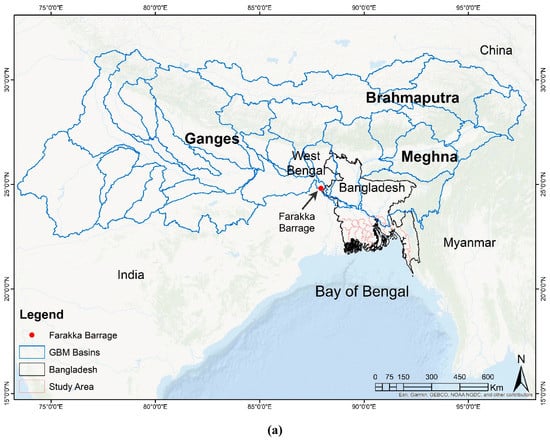
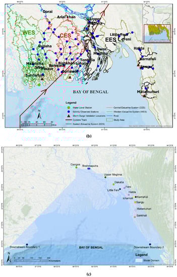
Figure 1.
(a) Ganges-Brahmaputra-Meghna (GBM) basins, the GBM delta, and the location of the Farakka barrage. (b) The study area with observed stations and calibration/validation locations. (c) The upstream and downstream boundaries of the model domain.
As topological and hydro-geomorphological characteristics are important to understand the SI process in any delta, this section summarizes such characteristics of the GBM delta in the Bangladesh coast. Based on geomorphologic and hydrodynamic characteristics, the coastal zone is divided into three distinct coastal systems, namely the Eastern Estuarine System (EES), the Central Estuarine System (CES), and the Western Estuarine System (WES) [38,39]. The EES consists of Lower Meghna, Tentulia, Lohalia, Little Feni, and Feni in one hand and Halda, Karnafuli, Sangu, and Matamuhuri of the Chittagong region in another hand (Figure 1b). The estuaries of the Chittagong region are flashy in nature, and tidal ranges are different from the other part of eastern coast (Lower Meghna, Tentulia, Lohalia, Little Feni, and Feni).
The combined flow of the three mighty rivers—the Ganges, the Brahmaputra, and the Meghna (commonly known as the GBM river systems and ranked as one of the largest river systems in the world)—carries the freshwater flow for the coastal region of Bangladesh. The Meghna estuary is an important estuary of the eastern coast, as the combined flow of the GBM river systems is mainly drained out to the ocean through this estuary [40]. The Tentulia and Meghna estuaries of the EES have a maximum width of 3–10 km and 23–25 km, respectively, near the estuary mouth, compared to other estuaries that vary between 0.6–1.5 km. The CES consists of the Bishkhali, Baleswar, and Buriswar estuaries (Figure 1b). In the CES, the width of the estuary near the mouth varies between 1–8 km, with the highest being in the Baleswar estuary. The CES region is relatively shallow, and the rivers and channels flowing to the bay change their course rapidly [41]. The CES receives its freshwater from spill channels of the Meghna estuary as well as through the Arial Khan River, which is mainly bifurcated from the Ganges-Brahmaputra Rivers. The floodplain of the eastern and central coasts are mainly plain land, whereas the Chittagong region consists of hills. It has been observed that the Lower Meghna estuary, of the eastern to the central coast, experienced the most disastrous effects of tropical cyclones and storm surges in the world and is very vulnerable to such events [40]. The WES consists of the interconnected estuaries of Sundarban, including the Rupsha, Shibsa, Passur, and Malancha estuaries, as well as all other cross-connecting estuaries [38] (Figure 1b). Rupsha and Passur have the maximum width at the estuary mouth, varying between 1–5 km [42], and other criss-cross interconnected estuaries are less than 1 km. The topography is very low and flat here. Tide is dominant in the Passur-Shibsa river systems, and a very strong salinity intrusion occurs there [43]. The region is also known as a stable region, as the forest (the Sundarban) covers a large part of this estuarine system. Freshwater flow is lowest in the western coast. The Gorai River mainly carries the fresh water in the western region from the Ganges River. However, the freshwater flow of the Gorai has been decreasing significantly over the years, especially during the dry season due to the Farakka barrage, a barrage across the Ganges River in India (Figure 1a) [44].
The coastline of Bangladesh is characterized by a wide continental shelf, especially at the eastern part. Tidal levels are amplified by the combined effect of wind force and the shape of the continental shelf [43]. The flow distribution in the study area was determined by the combined action of tides and freshwater flow. Tides in the coastal and estuarine areas of Bangladesh are semi-diurnal in nature [43]. Flierl et al. [45] found that the inland and offshore islands of Bangladesh are low lying and very flat, and their mean height above sea level is less than 3 m. The normal tidal range is about 3 m near the Indian border in the west, and it gradually becomes higher to the east (central coast) to about 5m in the mouth of the Meghna estuary [43] before decreasing south-eastward [46]. River salinity in the estuaries of the Bangladesh coast varies seasonally and has been observed to be high in the dry season and low in the monsoon season [1,29].
3. Methodology
The Delft3D open-source hydrodynamic and salt-transport model was selected to simulate salinity transport in estuaries, as it is a widely-used open source numerical modeling system [47,48]. The Delft3D depth average model solves the continuity and momentum equations for an incompressible fluid, adopts a structured grid, and performs the spatial discretization of the equations using a cell-centered finite difference method [49,50]. For this study, variable grid sizes were chosen in estuaries and oceans in such a way so that a finer resolution (186–243 m) lied in the inland and in the estuarine system that covers the study area satisfactorily, whereas a coarser resolution (1100–1700 m) was used in the ocean. Measured discharges upstream in the Ganges, Brahmaputra, and Meghna rivers and tidal water levels in the ocean were specified as upstream and downstream boundaries (Figure 1c). Measured discharge data were collected from the Bangladesh Water Development Board (BWDB) for the year of 2011 (a dry year which is considered a base year for this study). The downstream tidal water level boundaries for 2011 were specified by using the global ocean tide model ‘NAO-tide’ that used the Nao 99b tidal prediction system considering 16 major tidal constituents [27,51]. The bathymetry of the Bay of Bengal was generated using the open-access bathymetry data produced by the General Bathymetric Chart of the Oceans (GEBCO). The inland ground elevation data were collected from the Water Resources Planning Organization of Bangladesh (WARPO) [29]. The measured cross-sectional data for each of the estuary in the estuarine systems of the GBM delta at selected locations were surveyed by the ESPA delta (http://www.espa.ac.uk) and DECCMA (www.deccma.com) projects. For the salinity model, a constant sea salinity of 35 ppt for the Bay of Bengal [38] was specified as a sea boundary condition, and a constant sea salinity of 0 ppt for fresh water was specified for the upstream condition. For the cyclone-generated storm surge model, SIDR (made landfall in the central coast, 2007) was selected, as this cyclone is representative of a high-intensity cyclone, as well as landfall time synchronized with a typical maximum salinity period. An SIDR track was collected from the Indian Meteorological Department (www.imd.gov.in). This research used a ‘generated’ SIDR scenario by changing the landfall time (the actual SIDR landfall was on 15 November; the usual cyclone season in the Bangladesh coast is April–May and October–November) of SIDR to be in the maximum salinity period, i.e., April 15. The wind and pressure field of cyclone SIDR was generated by using the Delft Dashboard, which was coupled with salinity model (through the Delft3D interface). The simulation period for salinity intrusion coupled with the storm surge model was two years, from which the one year’s simulation result was used to attain a stable initial condition for the second year’s simulation. The time step used in the model simulation was 10 minutes.
3.1. Model Calibration and Validation
The measured time series’ salinity magnitude data were discontinuous, and observed salinity stations did not cover the whole coast uniformly. Hence, comparison of time series of salinity magnitude between model simulation and measurement was not possible. Measured tidal water level data were available in specific locations from the Bangladesh Inland Water Transport Authority (BIWTA). From this study perspective, three water level measurement locations representing three estuarine systems along the coast were initially selected, and data were collected from the BIWTA. However, due to poor data quality and unclear data [52], only one station was selected to compare the model simulated water level with measurements. The locations of salinity measurement stations and the only water level measurement station, which were used for model calibration/validation, is shown in Figure 1b.
To identify the sensitivity of the model, Principal Component Analysis (PCA) was conducted using water level, velocity (as a proxy to tidal excursion), roughness, and eddy diffusivity as input parameters. PCA gives a correlation matrix that identifies the principal components for a system [53]. The Pearson correlation coefficient was used to find the correlation matrix from which weights of the parameters were found that describe how much an indicator can explain a component vector [53]. The maximum weight of an indicator implies the highest sensitivity. From the PCA analysis, it was found that flow parameters (roughness and velocity) are the most sensitive parameters for the eastern and western coasts, whereas the transport parameter (eddy diffusivity) is the most sensitive for the central coast (Table 1).

Table 1.
Results of Principal Component Analysis.
For salinity model calibration, two parameters were used—roughness and eddy diffusivity. A larger value of roughness means more obstruction to the flow, whereas a larger value of eddy diffusivity means diffusive transport is dominating over convective transport. For the best performance of the model during calibration, values of roughness varied between 0.00025 at the ocean (considered as large water body) and 0.025 at the estuaries (where the flow faces more resistance than the ocean). Values of eddy diffusivity varied from 50 m2/s to 1000 m2/s (mode of transport varies from convective to diffusive depending on the location of estuaries) within the estuaries and around 250 m2/s at the ocean (mainly convective transport). The same parameter values obtained during calibration were used during model validation.
3.1.1. Visualization of Model Performance during Calibration and Validation
The calibration result of the salinity model is visualized in Figure 2a–d. The calibration result shows a comparison of the spatial distribution of maximum salinity between the model simulation and measurement. To ensure a one-to-one comparison between the model and measurement, the model values were extracted only from the locations where measured data were available (see Figure 1b). The filled contour is shown in Figure 2a,b and was drawn by using the salinity values based on the locations shown in Figure 1b and the corresponding scatter plot in Figure 2c. The scatter plot of water level for one measurement location (Figure 1b) is shown in Figure 2d. The degree of scattering was measured by the 45º line (Figure 2c,d). The comparison shows the R2 value for the salinity comparison as 0.8469 and the R2 value for the water level comparison as 0.6123 (Figure 2c,d). After calibrating the model for the year 2011, the model was validated for the year 2010, (2010 is considered as an average flood year [54]) and the result is shown in Figure 3a–c). The R2 value for the scattered salinity plot is 0.855 (Figure 3c). After visualizing both the calibration and validation results, it can be qualitatively said that the model performance, when viewed for the entire study area, is “acceptable.”
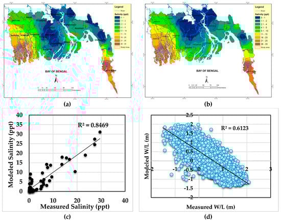
Figure 2.
Calibration result of salinity model that shows comparison of maximum salinity values and water level in one location in the study area during the year 2011. The result shows (a) measured and (b) modeled simulated salinity values in ppt. (c) Measured salinity vs. modeled salinity and (d) measured water level vs. modeled water level.
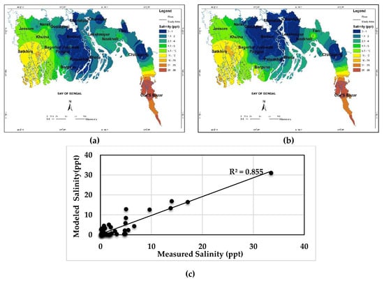
Figure 3.
Validation result of salinity model that shows comparison of maximum salinity values in the study area during the year 2010. The result shows (a) measured and (b) modeled simulated salinity values in ppt. (c) Measured salinity vs. modeled salinity.
3.1.2. Quantification of Model Performance
To quantify the qualitative visual performance of the model, 8 statistical indicators—the mean, standard deviation (STDEV), mean absolute error (MAE), root mean square error (RMSE), percent bias (PBIAS), Nash-Sutcliffe efficiency indicator (NSE), ratio of the RMSE between simulated and observed values to the standard deviation of the observations (RSR), and coefficient of determination (R2)—were calculated, and their “acceptable” ranges (which were reported in different literatures) are shown in Table 2. These indicators are generally used as model evaluation statistics [55,56,57,58,59]. Out of these 8 statistical indicators, the mean and STDEV represent descriptive statistics that quantitatively express the main feature of a dataset [60]. When the difference between these two indicators is “small” between the model and measured values, the main features of the model data and the measured data are similar. However, this does not guarantee that the spatial distribution of the model and measured data is also similar. The other six indicators (MAE, RMSE, PBIAS, NSE, RSR, and R2) are used to quantify the similarity. Among these six indicators, two indicators (MAE and RMSE) are considered error indicators, and the remaining four are considered dimensionless indicators [61]. Error indicators quantify the deviation in the units of the data of interest, whereas dimensionless indicators give a relative model evaluation assessment [57]. Table 2 shows the calibration and validation results for each of the estuarine systems separately (see Figure 1a), as well as for the entire system of the study area; when no reported acceptable range is found in the literature (Mean, STDEV and MAE), ranges were assumed (Table 2). The final evaluation shows that the model result is acceptable for individual estuarine systems as well as for the entire study domain (as 8 out of 8 are in the acceptable range for the entire study domain) (Table 2).
Table 2.
Statistical indicators showing the model performance during calibration and validation.
3.2. Descriptions of Scenarios
Climate scenarios were developed for three main events that affect SI in the GBM Delta [30]. Studies suggested that salinity ingress is likely to be more severe in the future since (a) reduced upstream discharge, as flows from rivers in the Himalayas are predicted to decrease, (b) sea levels are predicted to rise gradually, and (c) extreme events (i.e., cyclones and storm surges) are expected to be intensified in the changing climate [1,65,66]. As this research aimed to represent the extremes of salinity intrusion, scenarios were developed in such order. Upstream discharge reduction scenarios considered the dry season in driest condition (reducing both the monsoon and dry season flow). Sea level rise is also considered extreme limits of IPCC AR5 [67] and SIDR like high strength cyclone is chosen to examine its effect on salinity intrusion. Scenarios are summarized in Table 3.
Table 3.
Climate scenarios.
3.2.1. Reduced Discharge
Global Climate Models (GCMs) for the GBM basin projected discharges in the century scale and mentioned that upstream discharge reduction is a likely scenario in the future due to human intervention. However, GCM studies did not consider discharge reduction while projecting the scenarios [69,70,71]. This research considers a generated extreme case of upstream discharge reduction over the whole year that has the potential to leave an impact on salinity intrusion along the Bangladesh coast. A reduction for each discharge scenario was derived by subtracting the corresponding discharge dataset from its standard deviation value (where resulting negative values were kept as the actual value of dataset) (Table 3). The comparison of the base and scenarios are shown in Figure 4.
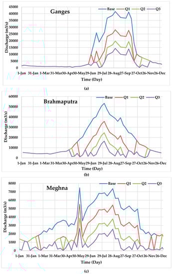
Figure 4.
Reduced discharge scenarios from base condition for (a) the Ganges, (b) Brahmaputra, and (c) Meghna rivers.
Discharge reduction methods exhibit a satisfactory match with true data (Figure 5). The extreme flood year of 1998 [72] was reduced in the same way as Table 3 and was examined to find a match with actual data of the dry year 2011 [68] (Figure 5). This represents that when the discharge of a flood year is reduced using standard deviation, it will match the magnitude of discharge (in terms of peak value) of a dry year. In the climatic condition when a dry year will be drier, a further reduction of discharge (like Figure 4) is a likely scenarios.
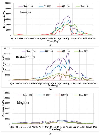
Figure 5.
Reduced discharge scenarios from base 1998 for (a) the Ganges, (b) Brahmaputra, and (c) Meghna rivers.
3.2.2. Sea Level Rise
The AR5 of the IPCC predicted a global rise of mean sea level by 0.52–0.98 m by the year 2100 [67]. Based on the IPCC projection, the maximum sea level rise in the Bay of Bengal is slightly higher (0.02 m) than the maximum global average. This research followed AR5 to construct SLR scenarios, and, after introducing the local correction for the Bay of Bengal, the maximum sea level rise was considered 1.0 m, with incremental changes of 0.25 m and 0.50 m towards the end of the century. With the base mean tide level of zero sea level rise, 0.25 m, 0.50 m, and 1.00 m were added to the mean of the base tide level to have the sea level rise scenarios. For a yearly cycle when neap-spring and seasonal variability was considered, tidal range (TR) in the sea varies between 0.25 m and 2.6 m.
3.2.3. Cyclonic Scenario
Among the recent cyclones, according to the Indian Meteorological Department (IMD) scale, SIDR (2007) was an extremely severe cyclonic storm (maximum wind speed 215–260 km/hr) which carried a significant amount of saline water through the estuaries and left severe impacts on the affected area, in terms of the salinity problem [73]. Considering the impact and susceptible landfall location [1,40,74], SIDR was chosen as the base cyclone by keeping the same wind speed and landfall location (which is named “Base Cyclone” in Table 3) to identify the effects of salinity intrusion due to a high strength cyclonic event. The effect of the extreme cyclonic condition was analyzed by considering an increase of wind speed of SIDR in future climatic conditions. For “Cyc-Scenario,” the standard deviation value (wind speed) of the “Base Cyclone” was added to the SIDR data (Figure 6) (Table 3).
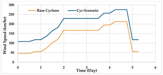
Figure 6.
Cyclonic scenarios.
When wind speed of a relatively weaker cyclone like ‘MORA’ (May 2017; landfall between the fishing port of Cox’s Bazar and the port city Chittagong) was increased following the same method of Figure 6, it was observed that after the 4th increment from base data, ‘W4-MORA’ matched with SIDR data (Base cyclone) (Figure 7). After one standard deviation increment of SIDR data (Base cyclone), ‘W1-SIDR’ (Cyc-Scenario) was derived, SIDR was observed to be relatively close to another cyclone named here as “Base-1991” that hit the Bangladesh coast in 1991 (Figure 7). Hence, it can be said that the method of wind increment represents the likely scenario for the cyclonic condition.
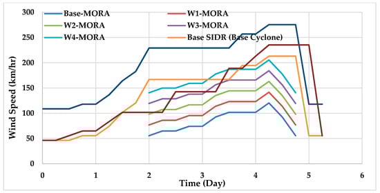
Figure 7.
Wind increment from Base-MORA and Base SIDR.
4. Result and Discussion
4.1. Base Salinity Condition from Measurement
The measured salinity value in the GBM delta indicates that the upper eastern-central coast (EES-CES) was relatively fresh (0–1 ppt) in the base year (2011) (Figure 8). The western coast had very high salinity, as its salinity magnitude was greater than 15 ppt. This spatial variation of salinity along the Bangladesh coast can be correlated with the fresh water–salt water interaction through three distinct estuarine systems (EES, CES, and WES) [38]. The EES receives the maximum amount of freshwater flow through the Meghna estuary, whereas the WES receives the minimum, and the CES receives an amount in-between the two [38].
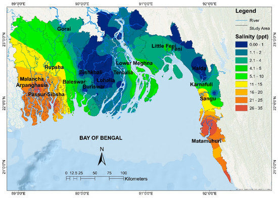
Figure 8.
Base salinity in 2011, from measurement.
4.2. Impact of Reduced Upstream Discharge on Salinity Intrusion
Reduced upstream discharges (Q1, Q2, Q3) were responsible for the gradually increment of the salinity magnitude all along the coast depending on the discharge scenarios (Figure 9). The freshwater zone (0–1ppt) of the EES (Lower Meghna, Tentulia) and the CES gradually disappeared with the reduction of freshwater flow (Figure 9). The maximum impact was in the WES, which already had the maximum salinity in the base condition (Figure 8). The salinity magnitude increased by 8–9 ppt in the WES, depicting a further landward intrusion (Figure 10).
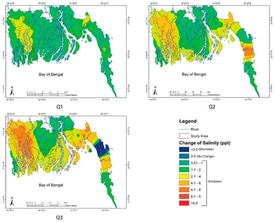
Figure 9.
Change of salinity magnitude for reduced discharge (Q1, Q2, and Q3).
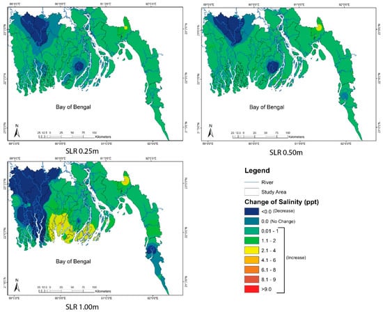
Figure 10.
Change of salinity magnitude for SLR (0.25, 0.50, 1.00 m).
4.3. Impact of Sea Level Rise on Salinity Intrusion
The salinity magnitude increased less than 1 ppt due to 0.25 m and 0.50 m SLR conditions (Figure 10). A 1.00 m sea level rise pushed the saline front upward in the central-eastern coasts and increased the salinity magnitude by 2–4 ppt in the seaward part (Figure 10). The intrusion occurred up to a certain distance inland and decreased gradually. The highest effect of SLR was observed in the central coast that was relatively fresh in the base condition. In general, the impact of SLR is less than reduced upstream flow (Figure 9 and Figure 10).
Due to SLR, the freshwater zone of the upper western coast spread out toward the coastline that resulted in a decreasing salinity magnitude (less than the base) (Figure 10). This might be due to the backwater effect, which indicates a large amount of stagnant fresh water from upstream resulting in fluvial flooding [40,75]. The backwater effect is the propagation of the effect of SLR upstream, which can be expressed as changes in water levels near the river mouth [40,75]. Complex hydrodynamics lie behind this change, which depends on the volume of water entering and exiting in an estuary (flood volume and ebb volume) during tidal cycles. An increased freshwater volume due to the backwater effect (not from upstream flow) decreases the salinity magnitude in this region.
4.4. Impact of Cyclone on Salinity Intrusion
In the Northern Hemisphere, the right part of the cyclone track (facing in the direction which the cyclone is moving) is called the dangerous semi-circles because of the forward motion of the cyclone, for which onshore winds are observed to the right of the path [76], and higher wind-forcing creates higher surge heights [77].
This particular directional impact of wind of tropical cyclones (TCs) also takes effect in this study as the Base Cyclone (TC SIDR) and its Cyc-scenario had landfall at the eastern side of Sundarbans, impacted (changes of salinity magnitude in a range of 4–9 ppt) mainly along the right part of the landfall location of cyclones (Figure 11). The changes are prominent from the Baleswar River of the central coast to the Lower Meghna estuary of the eastern coast (see Figure 1b for locations and Figure 11 for impacts).
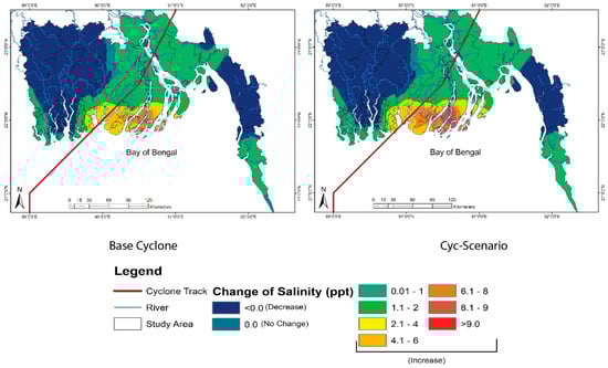
Figure 11.
Change of salinity magnitude for the Base Cyclone and the Cyc-Scenario.
4.5. Salinity Intrusion in Changing Climate
Changes of maximum salinity, corresponding tidal range, and flood velocity for three different scenarios (discharge reduction, SLR, and cyclonic scenarios), and for three estuaries of three different coasts (west, central, and east) are shown in Figure 12. SLR and cyclonic scenarios indicate varying impacts on different coasts. An increased flood velocity augments salinity magnitude along the east and central coasts during SLR. An increased salinity of approximately 5 ppt (in the central and east coasts) is associated with an increased flood tide velocity of 0.06 m/s. An increased flood velocity also contributes to an increased salinity in the east coast (where freshwater discharge is the highest) during the reduced discharge scenario. An increased tidal range causes a salinity increment along the central and eastern coasts during the cyclonic condition. It is to be noted here that the central and eastern coasts are considered the cyclone landfall locations in cyclone scenarios.
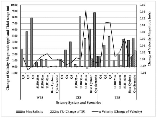
Figure 12.
Change of maximum salinity (Δ Max Salinity), tidal range (Δ TR), and flood tide velocity (Δ Velocity) along three coastlines. The changes denoted by Δ represents change from the base condition. The -ve values indicates reduction from base values and +ve values indicates increase from base values.
A discharge reduction gradually increases the salinity magnitude along the entire coast. However, this increased salinity is not always associated with an increased flood velocity (except in the eastern-central coast, which has the maximum freshwater flow). This shows that an increase of flood velocity and the associated increase of salinity depends on a balance between ebb strength (a function of freshwater flow) and flood strength (a function of freshwater flow and tidal range). However, the equilibrium relation is obviously non-linear (Figure 12). This non-linearity may be caused by the potential energy components (water surface slope and bed slope) of the total energy gradients that drive the flow during a tidal cycle which also have impacts on the transport process [78].
When we analyzed each of the coasts separately (WES, CES, and EES), it was found that upstream reduced discharge is the main driving event for increased the salinity intrusion along the coast. SLR is the dominant event in the central coast, which is relatively shallow compared to the west and east coasts. The cyclone is the dominant event in the central and east coasts (close to landfall location). Cyclones also cause a change in the tidal range for a short duration during the movement of cyclones along the coast.
4.6. Salinity Intrusion in Extremely Severe Climatic Condition
Though the main research question of this paper is to find the dominant climate change event for salinity intrusion in the GBM delta, it is interesting to examine the impact of a climatic condition where all the extreme climate change scenarios considered in this study—reduced upstream discharge scenario Q3, SLR 1.0 m, and Cyc-Scenario (Section 3.2, Table 3)—occur at a time. This kind of event is unlikely to occur but not impossible. Due to the multiplier effect, this extreme climate change scenario creates an extreme increase of salinity in the region (Figure 13). Except in the upper western estuarine systems where the backwater effect determines the salinity intrusion process (described in Section 4.3), all other estuaries in the system experience an increased salinity magnitude from 4 ppt to 9 ppt (Figure 13).
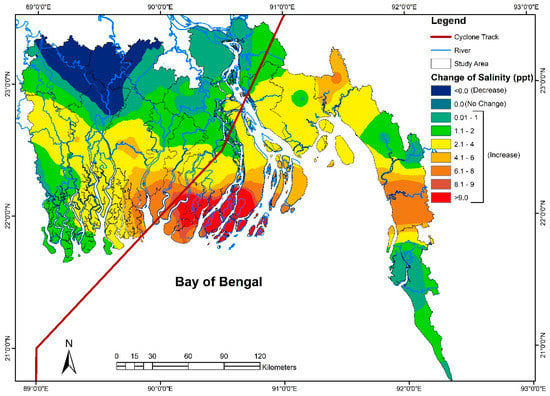
Figure 13.
Change of salinity magnitude for an extremely severe climatic condition.
5. Conclusions
Considering three dominant climatic events of salinity intrusion, this study found that the reduced discharge causes an increase of salinity in all types of the coast. The impact of SLR is more prominent in a relatively shallower coast. Salinity intrusion due to cyclonic scenarios is confined close to the cyclone landfall location. Cyclonic events increase the tidal range for a short duration during the passage of a cyclone along the coast. The relationship between flood velocity and an increase in salinity is non-linear for all types of coast
Scientific studies in the low lying deltaic region (for example, in the Bangladesh coast) had mentioned with great care that SLR (or the rising tide level) is going to affect the coastal area severely by pushing more tidal water inland, inundating more coastal areas; in another way, this effect can be interpreted as bringing more salinity intrusion along the coast [1,79,80,81]. Such emphasized scientific research of SLR impact on salinity intrusion results in more focus on governmental or non-governmental projects for the mitigation or adaptation of SLR. While there is no doubt of the increased salinity intrusion due to SLR, this research emphasis downplays the effects of reduced discharge conditions. This raises an important question: Whether the policymakers should only focus on SLR (which is a global phenomenon) or should focus on ensuring the optimal flow of an estuary (which is a regional phenomenon) to push saline water back to the ocean. In this era of globalization and anthropogenic development, barrages and dams are parts of river development and control projects, and, keeping this in mind, it is necessary to check whether such projects are interfering with the upstream flow that contributes to reducing downstream salinity of a delta. By investigating this idea, we might end up having much more devastating results than a 1.0 m SLR and increased cyclone frequency and intensity. Salinity intrusion is a lengthy process, and it is uncertain whether intruded salinity will reduce completely. Even if it reduces, it will be another very long term process. As such, with increasing salinity intrusion, it would be difficult to minimize the adverse effects. Keeping this fact in mind, regional cooperation in the basin scale is necessary so that the present upstream discharge will not reduce in the future.
Author Contributions
Conceptualization, R.A., T.Z.A., and M.S.; data curation, R.A. and T.Z.A.; formal analysis, R.A. and T.Z.A.; funding acquisition, M.M.R.; investigation, R.A., T.Z.A., M.N.S., and M.M.; methodology, R.A., T.Z.A., and M.A.; validation, R.A., T.Z.A., and M.A.; supervision, A.H.; Visualization, R.A., T.Z.A., and A.S.M.A.A.A.; writing—original draft, R.A. and T.Z.A.; writing—review & editing, R.A., T.Z.A., M.S., and A.H.
Limitations
This research did not consider the hydro-morphologic and topographic parameters causing salinity intrusion. This study focused on identifying a dominant event of salinity intrusion on which delta management plan should be focused on. This study was outlined to examine extreme condition of salinity intrusion due to three main climatic events through Delft3D modeling by acknowledging: “All models are wrong, but some are useful” [82].
Funding
International Development Research Centre: 107642.
Acknowledgments
This work was carried out under the Collaborative Adaptation Research Initiative in Africa and Asia (CARIAA), with financial support from the UK Government’s Department for International Development (DFID) and the International Development Research Centre (IDRC), Canada. The views expressed in this work are those of the creators and do not necessarily represent those of DFID and IDRC or its Board of Governors. Website: www.deccma.com.
Conflicts of Interest
The authors declare no conflict of interest.
References
- Dasgupta, S.; Huq, M.; Khan, Z.H.; Ahmed, M.M.Z.; Mukherjee, N.; Khan, M.F.; Pandey, K. Cyclones in a changing climate: The case of Bangladesh. Clim. Dev. 2014, 6, 96–110. [Google Scholar] [CrossRef]
- Nicholls, R.J.; Hutton, C.W.; Lázár, A.N.; Allan, A.; Adger, W.N.; Adams, H.; Wolf, J.; Rahman, M.; Salehin, M. Integrated assessment of social and environmental sustainability dynamics in the Ganges-Brahmaputra-Meghna delta, Bangladesh. Estuar. Coast. Shelf Sci. 2016, 183, 370–381. [Google Scholar] [CrossRef]
- Saito, Y. Deltas in Southeast and East Asia: Their evolution and current problems. In Proceedings of the APN/SURVAS/LOICZ Joint Conference on Coastal Impacts of Climate Change and Adaptation in the Asia–Pacific Region, APN, Kobe, Japan, 14–16 November 2000; pp. 185–191. [Google Scholar]
- De Souza, K.; Kituyi, E.; Harvey, B.; Leone, M.; Murali, K.S.; Ford, J.D. Vulnerability to climate change in three hot spots in Africa and Asia: Key issues for policy-relevant adaptation and resilience-building research. Reg. Environ. Chang. 2015, 15, 747–753. [Google Scholar] [CrossRef]
- Dearing, J.A.; Hossain, S. Recent Trends in Ecosystem Services in Coastal Bangladesh. Ecosyst. Serv. Well-Being Deltas 2018, 93–114. [Google Scholar] [CrossRef]
- Werner, A.D.; Bakker, M.; Post, V.E.; Vandenbohede, A.; Lu, C.; Ataie-Ashtiani, B.; Simmons, C.T.; Barry, D.A. Seawater intrusion processes, investigation and management: Recent advances and future challenges. Adv. Water Resour. 2013, 51, 3–26. [Google Scholar] [CrossRef]
- Wu, H.; Zhu, J.; Choi, B.H. Links between saltwater intrusion and subtidal circulation in the Changjiang Estuary: A model-guided study. Cont. Shelf Res. 2010, 30, 1891–1905. [Google Scholar] [CrossRef]
- Barlow, P.M.; Reichard, E.G. Saltwater intrusion in coastal regions of North America. Hydrogeol. J. 2010, 18, 247–260. [Google Scholar] [CrossRef]
- Neubauer, S.C. Ecosystem responses of a tidal freshwater marsh experiencing saltwater intrusion and altered hydrology. Estuaries Coasts 2013, 36, 491–507. [Google Scholar] [CrossRef]
- Yanosky, T.M.; Hupp, C.R.; Hackney, C.T. Chloride concentrations in growth rings of Taxodium distichum in a saltwater-intruded estuary. Ecol. Appl. 1995, 5, 785–792. [Google Scholar] [CrossRef]
- Craft, C.; Clough, J.; Ehman, J.; Joye, S.; Park, R.; Pennings, S.; Guo, H.; Machmuller, M. Forecasting the effects of accelerated sea-level rise on tidal marsh ecosystem services. Front. Ecol. Environ. 2009, 7, 73–78. [Google Scholar] [CrossRef]
- Werner, A.D.; Simmons, C.T. Impact of sea-level rise on sea water intrusion in coastal aquifers. Groundwater 2009, 47, 197–204. [Google Scholar] [CrossRef]
- Rosegrant, M.W.; Ringler, C.; McKinney, D.C.; Cai, X.; Keller, A.; Donoso, G. Integrated economic-hydrologic water modeling at the basin scale: The Maipo River basin. Agric. Econ. 2005, 24, 33–46. [Google Scholar] [CrossRef]
- Wang, B.; Zhu, J.; Wu, H.; Yu, F.; Song, X. Dynamics of saltwater intrusion in the Modaomen Waterway of the Pearl River Estuary. Sci. China Earth Sci. 2012, 55, 1901–1918. [Google Scholar] [CrossRef]
- Winn, K.O.; Saynor, M.J.; Eliot, M.J.; Elio, I. Saltwater intrusion and morphological change at the mouth of the East Alligator River, Northern Territory. J. Coast. Res. 2006, 137–149. [Google Scholar] [CrossRef]
- Antonellini, M.; Mollema, P.; Giambastiani, B.; Bishop, K.; Caruso, L.; Minchio, A.; Pellegrini, L.; Sabia, M.; Ulazzi, E.; Gabbianelli, G. Salt water intrusion in the coastal aquifer of the southern Po Plain, Italy. Hydrogeol. J. 2008, 16, 1541. [Google Scholar] [CrossRef]
- Zhang, E.; Savenije, H.H.; Wu, H.; Kong, Y.; Zhu, J. Analytical solution for salt intrusion in the Yangtze Estuary, China. Estuar. Coast. Shelf Sci. 2011, 91, 492–501. [Google Scholar] [CrossRef]
- Junot, J.A.; Poirrier, M.A.; Soniat, T.M. Effects of saltwater intrusion from the Inner Harbor Navigation Canal on the benthos of Lake Pontchartrain, Louisiana. Gulf Caribb. Res. 1983, 7, 247–254. [Google Scholar] [CrossRef]
- Qiu, C.; Zhu, J.R. Influence of seasonal runoff regulation by the Three Gorges Reservoir on saltwater intrusion in the Changjiang River Estuary. Cont. Shelf Res. 2013, 71, 16–26. [Google Scholar] [CrossRef]
- Han, Z.-C.; Cheng, H.-P.; Shi, Y.-B.; You, A.-J. Long-term predictions and countermeasures of saltwater intrusion in the Qiantang estuary. J. Hydraul. Eng. 2012, 2. [Google Scholar]
- Shaha, D.C.; Cho, Y.K.; Kim, T.W. Effects of river discharge and tide driven sea level variation on saltwater intrusion in Sumjin River estuary: An application of finite-volume coastal ocean model. J. Coast. Res. 2012, 29, 460–470. [Google Scholar] [CrossRef]
- Gong, W.; Shen, J. The response of salt intrusion to changes in river discharge and tidal mixing during the dry season in the Modaomen Estuary, China. Cont. Shelf Res. 2011, 31, 769–788. [Google Scholar] [CrossRef]
- Xu, H.; Lin, J.; Wang, D. Numerical study on salinity stratification in the Pamlico River Estuary. Estuar. Coast. Shelf Sci. 2008, 80, 74–84. [Google Scholar] [CrossRef]
- Feseker, T. Numerical studies on saltwater intrusion in a coastal aquifer in northwestern Germany. Hydrogeol. J. 2007, 15, 267–279. [Google Scholar] [CrossRef]
- Zhou, W.; Wang, D.; Luo, L. Investigation of saltwater intrusion and salinity stratification in winter of 2007/2008 in the Zhujiang River Estuary in China. Acta Oceanol. Sin. 2012, 31, 31–46. [Google Scholar] [CrossRef]
- Van Aken, H.M. Variability of the salinity in the western Wadden Sea on tidal to centennial time scales. J. Sea Res. 2008, 59, 121–132. [Google Scholar] [CrossRef]
- Sumaiya, H.A.; Rahman, M.; Elahi, W.E.; Ahmed, I.; Rimi, R.A.; Alam, S. Modelling Salinity Extremes in Bangladesh Coast. In Proceedings of the 5th International Conference on Water & Flood Management (ICWFM-2015), Dhaka, Bangladesh, 6–8 March 2015. [Google Scholar]
- Hussain, M.A.; Islam, A.; Hasan, M.A.; Bhaskaran, B. Changes of the seasonal salinity distribution at the Sundarbans coast due to impact of climate change. In Proceedings of the 4th International Conference on Water & Flood Management (ICWFM-2013), Dhaka, Bangladesh, 9–11 March 2013; pp. 637–648. [Google Scholar]
- Akter, R.; Sumaiya, S.; Rahman, M.; Ahmed, T.; Sakib, M.; Haque, A.; Rahman, M.M. Prediction of Salinity Intrusion due to Sea Level Rise and Reduced Upstream Flow in the GBM Delta. In Proceedings of the 20th Congress of the Asia Pacific Division of the International Association for Hydro Environment Engineering & Research (IAHR), Colombo, Sri Lanka, 28–31 August 2016. [Google Scholar]
- Bashar, K.E.; Hossain, M.A. Impact of sea level rise on salinity of coastal area of Bangladesh. In Proceedings of the 9th International River Symposium, Brisbane, Australia, 4–7 September 2006. [Google Scholar]
- Akhter, S.; Hasan, M.M.; Khan, Z.H. Impact of climate change on saltwater intrusion in the coastal area of Bangladesh. In Proceedings of the 8th International Conference on Coastal and Port Engineering in Developing Countries (COPEDEC 2012), Chennai, India, 20–24 February 2012. [Google Scholar]
- Bricheno, L.M.; Wolf, J.; Islam, S. Tidal intrusion within a mega delta: An unstructured grid modelling approach. Estuar. Coast. Shelf Sci. 2016, 182, 12–26. [Google Scholar] [CrossRef]
- Bhuiyan, M.J.A.N.; Dutta, D. Assessing impacts of sea level rise on river salinity in the Gorai river network, Bangladesh. Estuarine. Coast. Shelf Sci. 2012, 96, 219–227. [Google Scholar] [CrossRef]
- Mirza, M.M.Q. Effects on Water Salinity in Bangladesh. In The Ganges Water Diversion: Environmental Effects and Implications; Water Science and Technology Library; Springer: Dordrecht, The Netherlands, 2004; Volume 49, pp. 1–12. [Google Scholar] [CrossRef]
- Akter, R.; Sakib, M.; Rahman, M.; Sumaiya, S.; Haque, A.; Rahman, M.M.; Islam, R. Climatic and Cyclone Induced Storm Surge Impact on Salinity Intrusion along the Bangladesh Coast. In Proceedings of the 6th International Conference on the Application of Physical Modeling in Coastal and Port Engineering and Science (Coastlab 2016), Ottawa, ON, Canada, 11–13 May 2016; Available online: http://rdio.rdc.uottawa.ca/publications/coastlab16/coastlab6.pdf (accessed on 19 May 2019).
- WARPO. Coastal Development Strategy. In Ministry of Water Resources, Government of the People’s Republic of Bangladesh; Water Resources Planning Organization (WARPO): Dhaka, Bangladesh, 2006. [Google Scholar]
- Baten, M.A.; Seal, L.; Lisa, K.S. Salinity Intrusion in Interior Coast of Bangladesh: Challenges to Agriculture in South-Central Coastal Zone. Am. J. Clim. Chang. 2015, 4, 248–262. [Google Scholar] [CrossRef]
- Haque, A.; Sumaiya; Rahman, M. Flow Distribution and Sediment Transport Mechanism in the Estuarine Systems of Ganges-Brahmaputra-Meghna Delta. Int. J. Environ. Sci. Dev. 2016, 7, 22. [Google Scholar] [CrossRef]
- Munsur Rahman, A.H.; Siddique, M.K.; Rezaie, A.M.; Hafez, M.; Ahmed, R.J.; Darby, S.; Wolf, J.; Sarker, M.H.; Alam, S.; Ahmed, I.; et al. A preliminary assessment of the impact of fluvio-tidal regime on Ganges-Brahmaputra-Meghna delta and its impact on the ecosystem resources. In Proceedings of the International Conference on Climate Change Impact and Adaptation (I3CIA-2013), Gazipur, Bangladesh, 15–17 November 2013. [Google Scholar]
- Ali, A. Climate change impacts and adaptation assessment in Bangladesh. Clim. Res. 1999, 12, 109–116. [Google Scholar] [CrossRef]
- Sarker, M.H.; Akter, J.A.K.I.A.; Ferdous, M.R.; Noor, F.A.H.M.I.D.A. Sediment dispersal processes and management in coping with climate change in the Meghna Estuary, Bangladesh. In Proceedings of the Workshop on Sediment Problems and Sediment Management in Asian River Basins, Hyderabad, India, September 2009; IAHS: Hyderabad, India; pp. 203–218, Publication 349.
- Zaman, A.M.; Molla, M.K.; Pervin, I.A.; Rahman, S.M.; Haider, A.S.; Ludwig, F.; Franssen, W. Impacts on river systems under 2 °C warming: Bangladesh Case Study. Clim. Serv. 2017, 7, 96–114. [Google Scholar] [CrossRef]
- Komol, K.U. Numerical Simulation of Tidal Level at Selected Coastal Area of Bangladesh. Master’s Thesis, Bangladesh University of Engineering and Technology (BUET), Dhaka, Bangladesh, 2011. [Google Scholar]
- Brammer, H. Bangladesh’s dynamic coastal regions and sea-level rise. Clim. Risk Manag. 2014, 1, 51–62. [Google Scholar] [CrossRef]
- Flierl, G.R.; Robinson, A.R. Deadly surges in the Bay of Bengal: Dynamics and storm-tide tables. Nature 1972, 239, 213. [Google Scholar] [CrossRef]
- Pattullo, J. The seasonal oscillation in sea level. J. Mar. Res. 1955, 14, 25–39. [Google Scholar]
- Lesser, G.R.; Roelvink, J.A.; Van Kester, J.; Stelling, G.S. Development and validation of a three-dimensional morphological model. Coast. Eng. 2004, 51, 883–915. [Google Scholar] [CrossRef]
- Ranasinghe, R.; Swinkels, C.; Luijendijk, A.; Roelvink, D.; Bosboom, J.; Stive, M.; Walstra, D. Morphodynamic upscaling with the MORFAC approach: Dependencies and sensitivities. Coast. Eng. 2011, 58, 806–811. [Google Scholar] [CrossRef]
- Broomans, P. Numerical Accuracy in Solutions of the Shallow Water Equations. Master’s Thesis, Technical University of Delft, Delft, The Netherlands, 2003. [Google Scholar]
- Deltares. Simulation of Multi-Dimensional Hydrodynamic Flows and Transport Phenomena, Including Sediments. Delft3D-Flow, User Manual 2014, Version 3.15.34158; May 2014. Available online: https://www.lumes.lu.se/sites/lumes.lu.se/files/golam_sarwar.pdf (accessed on 21 May 2019).
- Matsumoto, K.; Takanezawa, T.; Ooe, M. Ocean tide models developed by assimilating TOPEX/POSEIDON altimeter data into hydrodynamical model: A global model and a regional model around Japan. J. Oceanogr. 2000, 56, 567–581. [Google Scholar] [CrossRef]
- Mondal, M.A.M.; Water, B.I. Sea level rise along the coast of Bangladesh; Report; Ministry of Shipping: Dhaka, Bangladesh, 2001.
- Jeong, D.H.; Ziemkiewicz, C.; Ribarsky, W.; Chang, R.; Center, C.V. Understanding Principal Component Analysis Using a Visual Analytics Tool; Charlotte Visualization Center, UNC Charlotte: Charlotte, NC, USA, 2009. [Google Scholar]
- BWDB. Annual Flood Report 2010, Flood Forecasting and Warning Centre, Processing and Flood Forecasting Circle; Bangladesh Water Development Board: Dhaka, Bangladesh, 2011.
- Willmott, C.J. On the validation of models. Phys. Geogr. 1981, 2, 184–194. [Google Scholar] [CrossRef]
- ASCE Task Committee on Definition of Criteria for Evaluation of Watershed Models of the Watershed Management Committee, Irrigation and Drainage Division. Criteria for evaluation of watershed models. J. Irrig. Drain. Eng. 1993, 119, 429–442. [Google Scholar] [CrossRef]
- Legates, D.R.; McCabe, G.J., Jr. Evaluating the use of “goodness-of-fit” measures in hydrologic and hydroclimatic model validation. Water Resour. Res. 1999, 35, 233–241. [Google Scholar] [CrossRef]
- Wang, X.; Melesse, A.M. Evaluation of the SWAT model’s snowmelt hydrology in a northwestern Minnesota watershed. Trans. ASAE 2005, 48, 1359–1376. [Google Scholar] [CrossRef]
- Parker, R.; Arnold, J.G.; Barrett, M.; Burns, L.; Carrubba, L.; Crawford, C.; Neitsch, S.L.; Snyder, N.J.; Srinivasan, R.; Williams, W.M. Evaluation of three watershed-scale pesticide fate and transport models. AWRA J. Am. Water Resour. Assoc. 2007, 43, 1424–1443. [Google Scholar] [CrossRef]
- Nicholas, J. Introduction to Descriptive Statistics; Mathematics Learning Centre, University of Sydney: Camperdown, NSW, Australia, 1999. [Google Scholar]
- Moriasi, D.N.; Arnold, J.G.; Van Liew, M.W.; Bingner, R.L.; Harmel, R.D.; Veith, T.L. Model evaluation guidelines for systematic quantification of accuracy in watershed simulations. Trans. ASABE 2007, 50, 885–900. [Google Scholar] [CrossRef]
- Singh, J.; Knapp, H.V.; Arnold, J.G.; Demissie, M. Hydrological modeling of the Iroquois river watershed using HSPF and SWAT 1. JAWRA J. Am. Water Resour. Assoc. 2005, 41, 343–360. [Google Scholar] [CrossRef]
- Santhi, C.; Arnold, J.G.; Williams, J.R.; Dugas, W.A.; Srinivasan, R.; Hauck, L.M. Validation of the swat model on a large RWER basin with point and nonpoint sources 1. JAWRA J. Am. Water Resour. Assoc. 2001, 37, 1169–1188. [Google Scholar] [CrossRef]
- Golmohammadi, G.; Prasher, S.; Madani, A.; Rudra, R. Evaluating three hydrological distributed watershed models: MIKE-SHE, APEX, SWAT. Hydrology 2014, 1, 20–39. [Google Scholar] [CrossRef]
- Ali, A. Vulnerability of Bangladesh to climate change and sea level rise through tropical cyclones and storm surges. In Climate Change Vulnerability and Adaptation in Asia and the Pacific; Springer: Dordrecht, The Netherlands, 1996; pp. 171–179. [Google Scholar] [CrossRef]
- Unnikrishnan, A.S.; Kumar, K.R.; Fernandes, S.E.; Michael, G.S.; Patwardhan, S.K. Sea level changes along the Indian coast: Observations and projections. Curr. Sci. 2006, 90, 362–368. [Google Scholar]
- IPCC; Church, J.A.; Clark, P.U.; Cazenave, A.; Gregory, J.M.; Jevrejeva, S.; Levermann, A.; Merrifield, M.A.; Milne, G.A.; Nerem, R.S.; et al. 2013: Sea Level Change. In Climate Change; The Physical Science Basis; Contribution of Working Group I to the Fifth Assessment Report of the Intergovernmental Panel on Climate Change; Stocker, T.F., Qin, D., Plattner, G.-K., Tignor, M., Allen, S.K., Boschung, J., Nauels, A., Xia, Y., Bex, V., Midgley, P.M., Eds.; Cambridge University Press: Cambridge, UK; New York, NY, USA, 2013. [Google Scholar]
- BWDB. Annual Flood Report 2011, Flood Forecasting and Warning Centre, Processing and Flood Forecasting Circle; Bangladesh Water Development Board: Dhaka, Bangladesh, 2012.
- Mohammed, K.; Saiful Islam, A.K.M.; Tarekul Islam, G.M.; Alfieri, L.; Bala, S.K.; Uddin Khan, M.J. Impact of High-End Climate Change on Floods and Low Flows of the Brahmaputra River. J. Hydrol. Eng. 2017, 22, 04017041. [Google Scholar] [CrossRef]
- Whitehead, P.G.; Barbour, E.; Futter, M.N.; Sarkar, S.; Rodda, H.; Caesar, J.; Butterfield, D.; Jin, L.; Sinha, R.; Nicholls, R.; et al. Impacts of climate change and socio-economic scenarios on flow and water quality of the Ganges, Brahmaputra and Meghna (GBM) river systems: Low flow and flood statistics. Environ. Sci. Process. Impacts 2015, 17, 1057–1069. [Google Scholar] [CrossRef]
- Fahad, M.G.R.; Saiful Islam, A.K.M.; Nazari, R.; Alfi Hasan, M.; Tarekul Islam, G.M.; Bala, S.K. Regional changes of precipitation and temperature over Bangladesh using bias-corrected multi-model ensemble projections considering high-emission pathways. Int. J. Climatol. 2018, 38, 1634–1648. [Google Scholar] [CrossRef]
- BWDB. Annual Flood Report 1999, Flood Forecasting and Warning Centre, Processing and Flood Forecasting Circle; Bangladesh Water Development Board: Dhaka, Bangladesh, 2000.
- Mahmuduzzaman, M.; Ahmed, Z.U.; Nuruzzaman, A.K.M.; Ahmed, F.R.S. Causes of salinity intrusion in coastal belt of Bangladesh. Int. J. Plant Res. 2014, 4, 8–13. [Google Scholar] [CrossRef]
- Quadir, D.A.; Iqbal, M.A. Investigation on the Variability of the Tropical Cyclones Impacting the Livelihood of the Coastal Inhabitants of Bangladesh; IUCN Contract No. IUCNB-Consult-069 & IUCNB-Consult-070; International Union for Conservation of Nature (IUCN): Dhaka, Bangladesh, 2008. [Google Scholar]
- Ikeuchi, H.; Hirabayashi, Y.; Yamazaki, D.; Kiguchi, M.; Koirala, S.; Nagano, T.; Kotera, A.; Kanae, S. Modeling complex flow dynamics of fluvial floods exacerbated by sea level rise in the Ganges–Brahmaputra–Meghna Delta. Environ. Res. Lett. 2015, 10, 124011. [Google Scholar] [CrossRef]
- Needham, H.; Keim, B.D. Storm surge: Physical processes and an impact scale. In Recent Hurricane Research-Climate, Dynamics, and Societal Impacts; InTech: London, UK, 2011. [Google Scholar]
- Hussain, M.A.; Tajima, Y.; Hossain, M.A.; Das, P. Impact of Cyclone Track Features and Tidal Phase Shift upon Surge Characteristics in the Bay of Bengal along the Bangladesh Coast. J. Mar. Sci. Eng. 2017, 5, 52. [Google Scholar] [CrossRef]
- Esposito, C.R.; Georgiou, I.Y.; Kolker, A.S. Hydrodynamic and geomorphic controls on mouth bar evolution. Geophys. Res. Lett. 2013, 40, 1540–1545. [Google Scholar] [CrossRef]
- McGranahan, G.; Balk, D.; Anderson, B. The rising tide: Assessing the risks of climate change and human settlements in low elevation coastal zones. Environ. Urban. 2007, 19, 17–37. [Google Scholar] [CrossRef]
- Shamsuddoha, M.; Chowdhury, R.K. Climate Change Impact and Disaster Vulnerabilities in the Coastal Areas of Bangladesh; Coast Trust: Dhaka, Bangladesh, 2007. [Google Scholar]
- Sarwar, M.G.M. Impacts of Sea Level Rise on the Coastal Zone of Bangladesh. 2005. Available online: https://www.lumes.lu.se/sites/lumes.lu.se/files/golam_sarwar.pdf (accessed on 19 May 2019).
- Box, G.E. Robustness in the strategy of scientific model building. Robust. Stat. 1979, 201–236. [Google Scholar] [CrossRef]


© 2019 by the authors. Licensee MDPI, Basel, Switzerland. This article is an open access article distributed under the terms and conditions of the Creative Commons Attribution (CC BY) license (http://creativecommons.org/licenses/by/4.0/).