Modeling the Impact of Climate Change on Water Availability in the Zarrine River Basin and Inflow to the Boukan Dam, Iran


Abstract
:1. Introduction
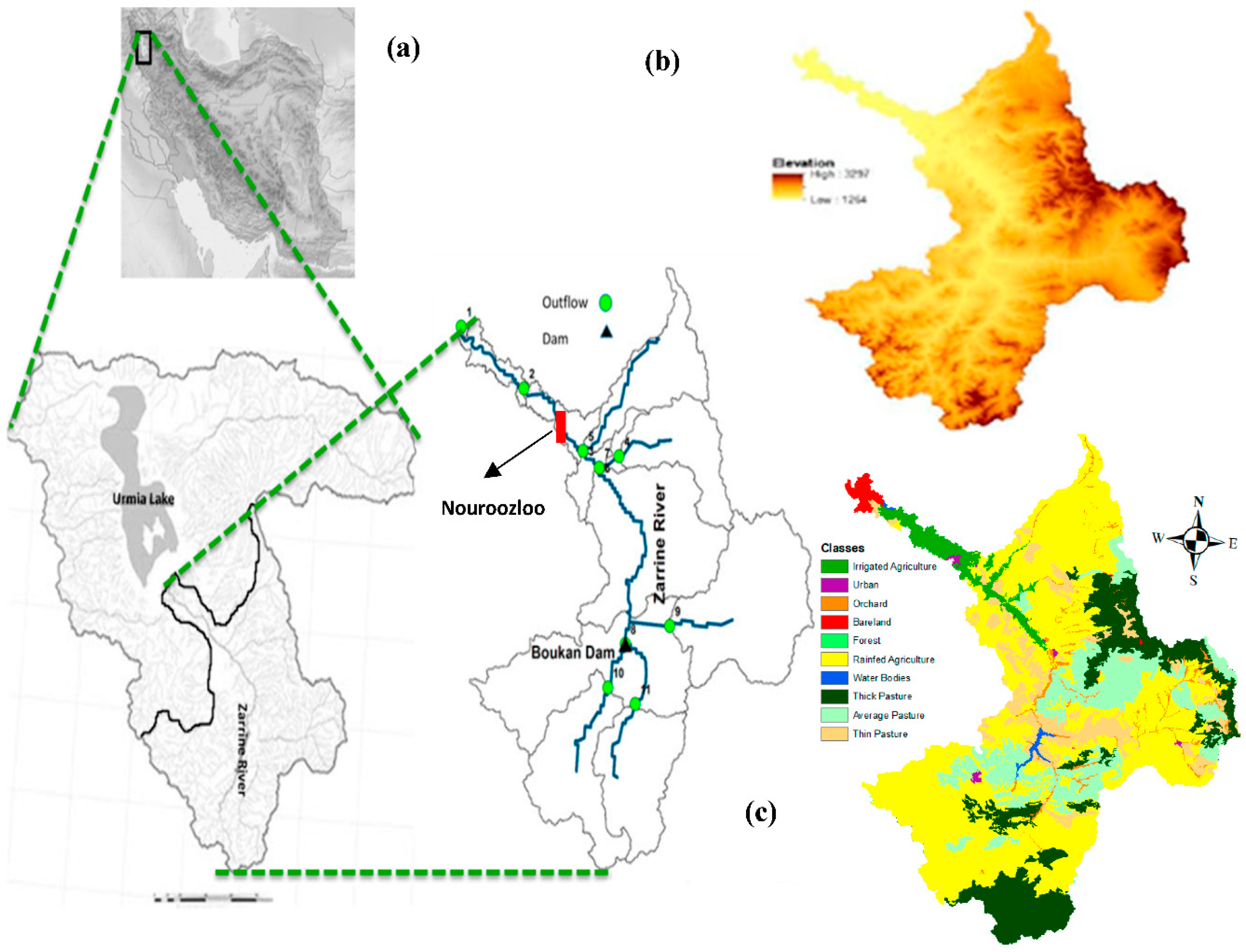
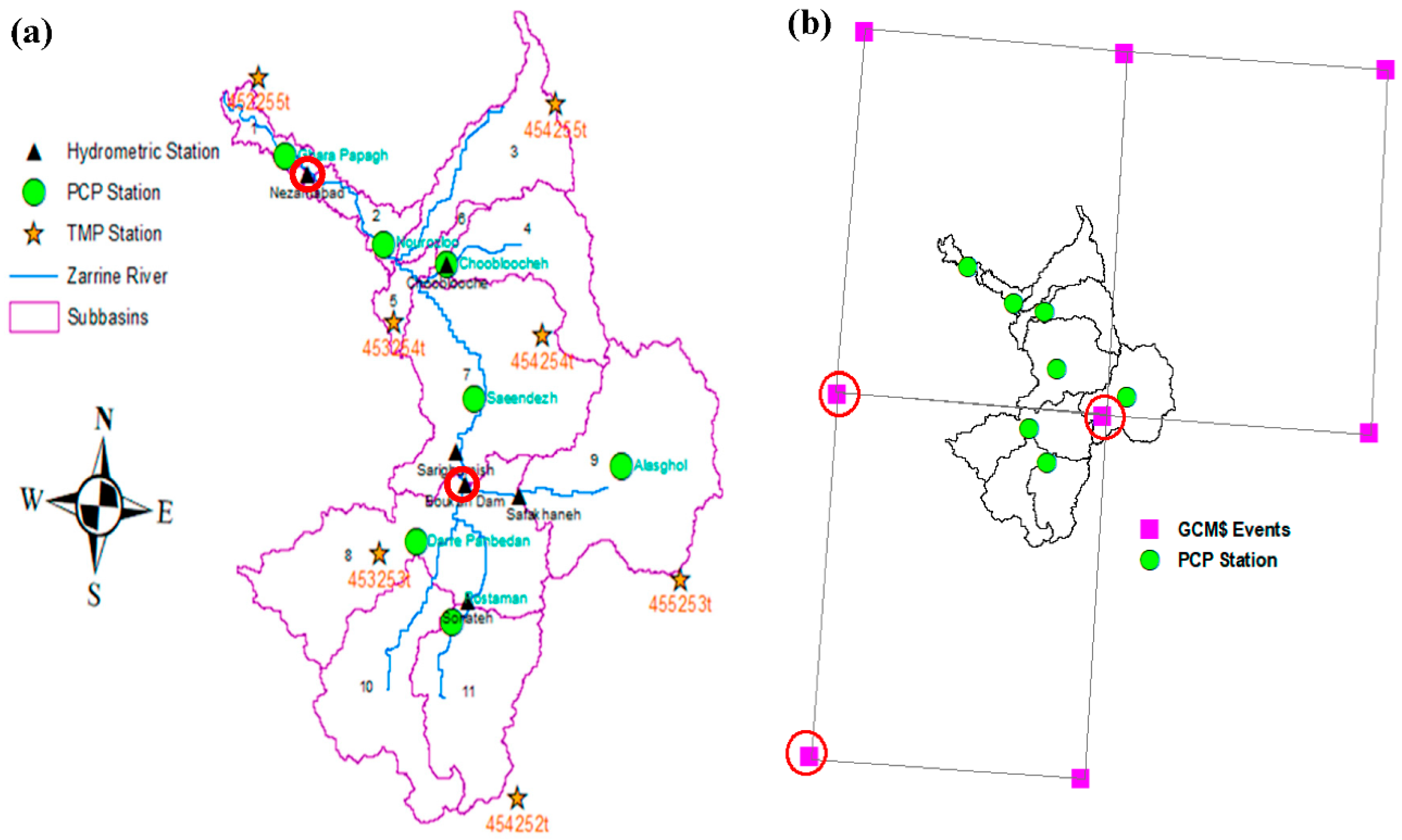
2. Study Area
3. Materials and Methods
3.1. Hydrological Simulation Model SWAT
3.1.1. Theoretical Concepts of the SWAT-Model
3.1.2. Model Setup
3.1.3. Calibration, Validation and Sensitivity Analysis
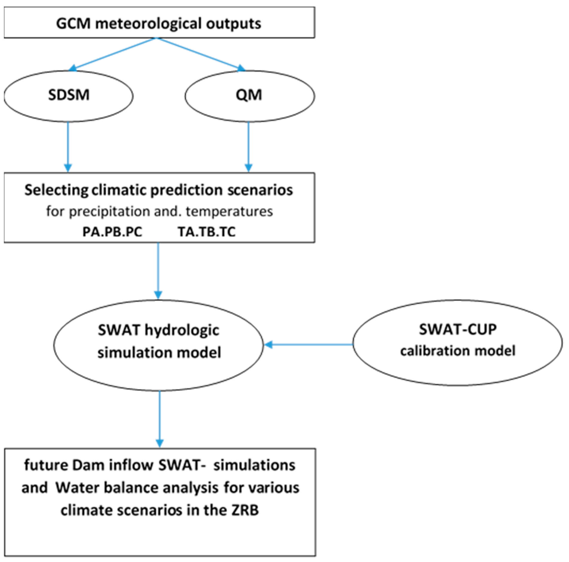
3.2. Climate Change Scenarios and Predictions
3.2.1. GCM-Selection
3.2.2. SDSM- and QM - Downscaling of Climate Predictors
4. Results and Discussion
4.1. SWAT-CUP Sensitivity Analysis
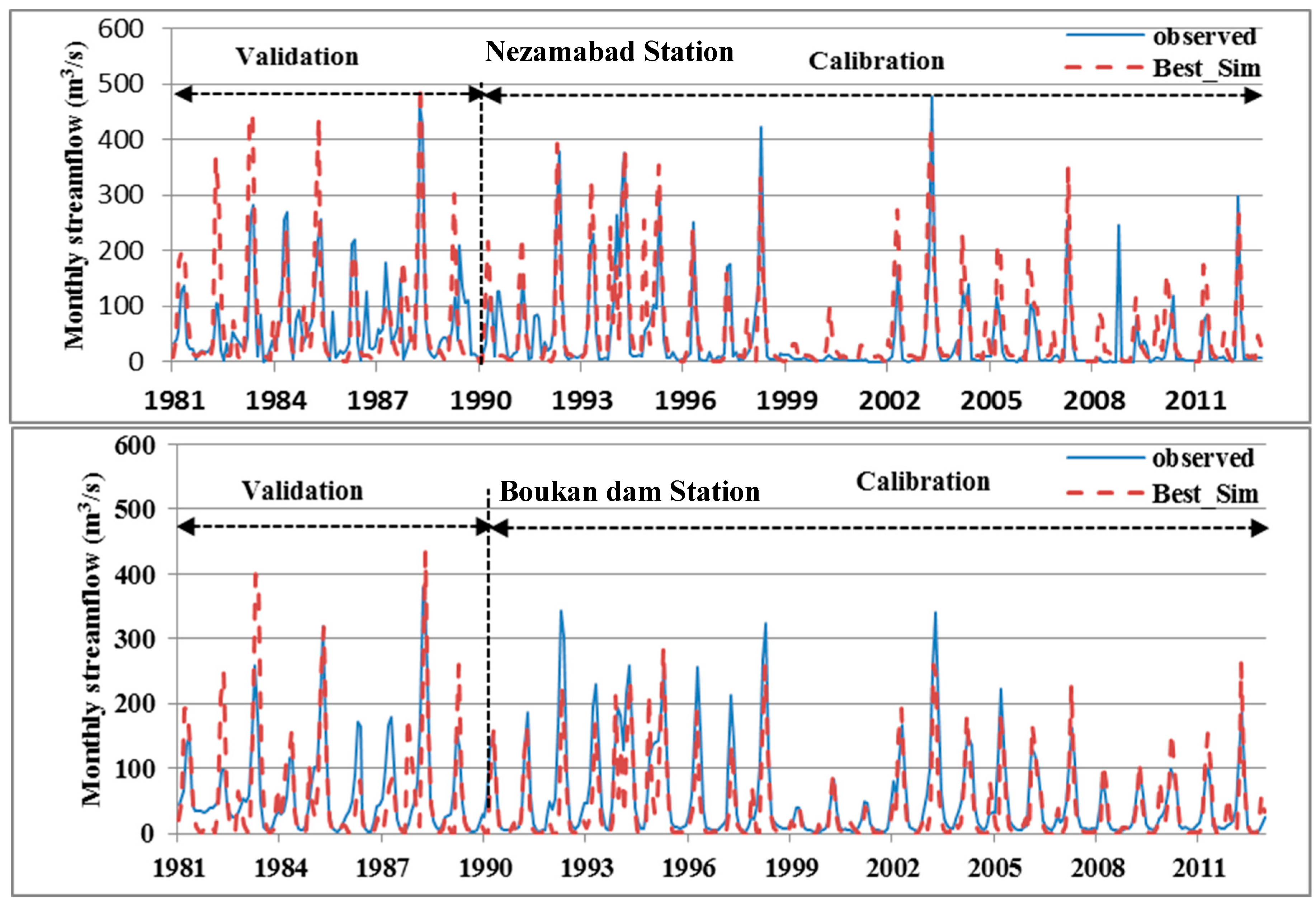
4.2. SWAT-Model Calibration and Validation
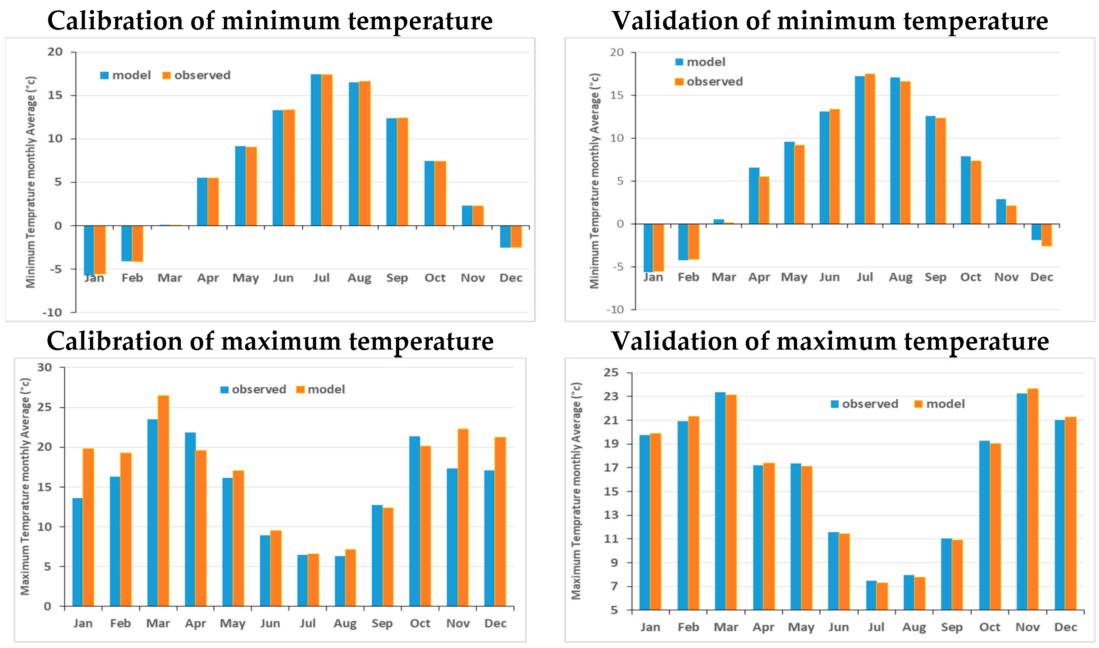
4.3. SDSM- Downscaling of CanESM2- Historical Temperatures
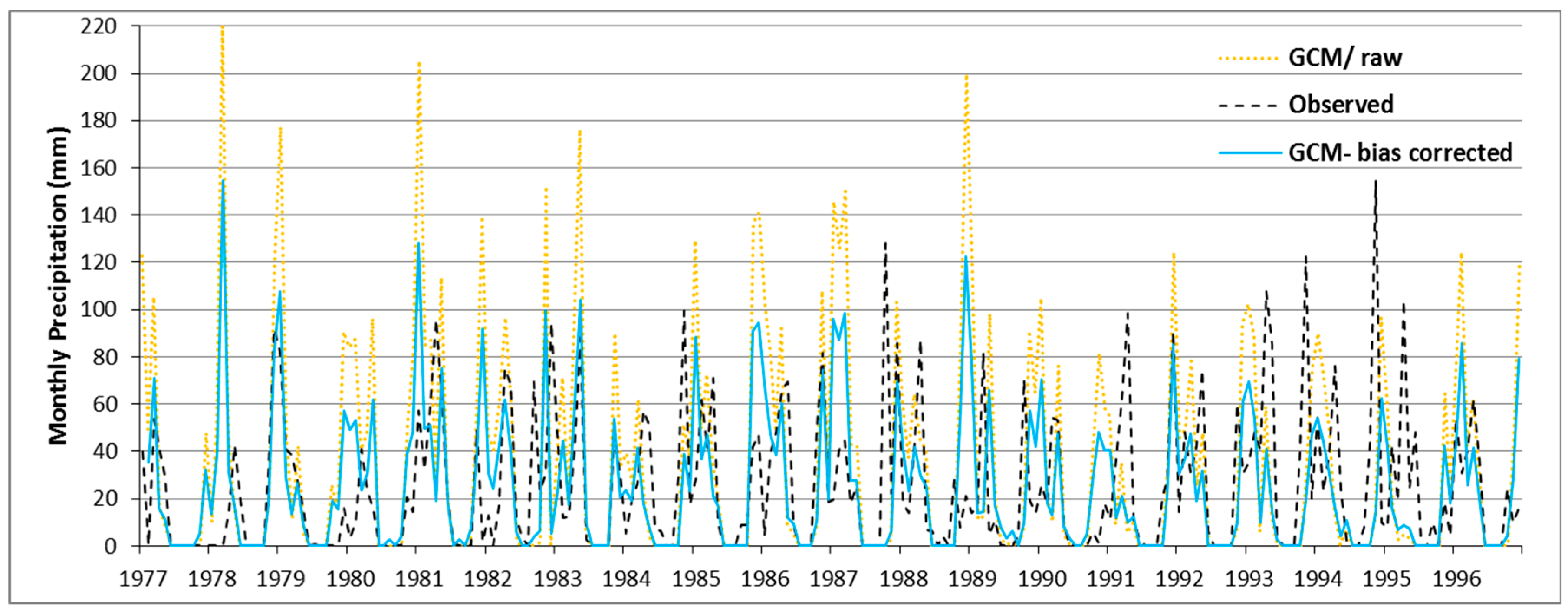
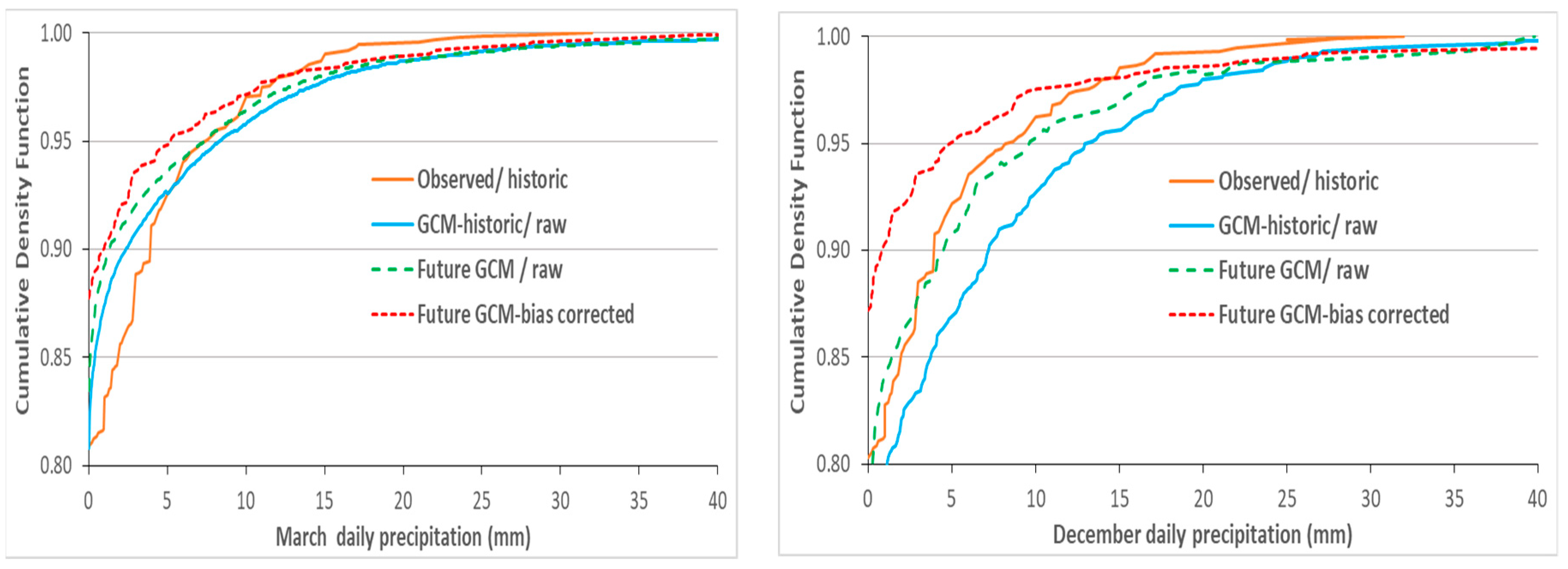
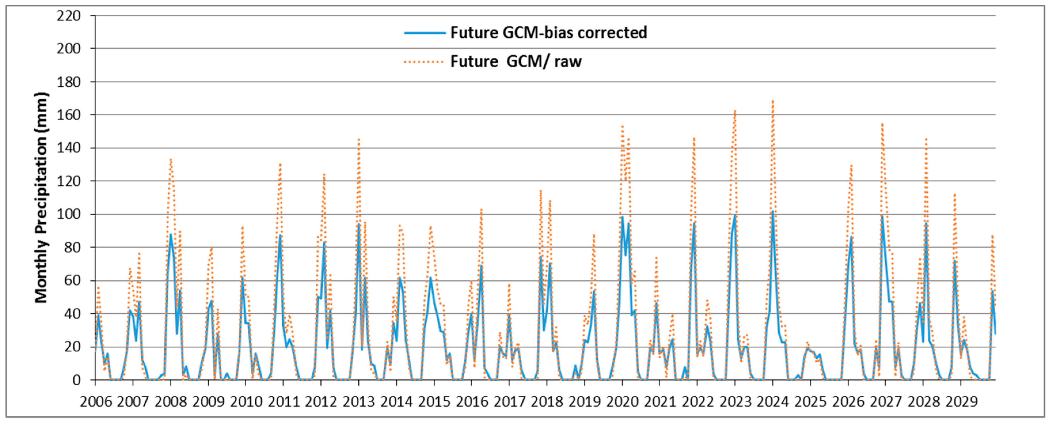
4.4. QM-Downscaling of MPI-ESM-LR Precipitation Predictors
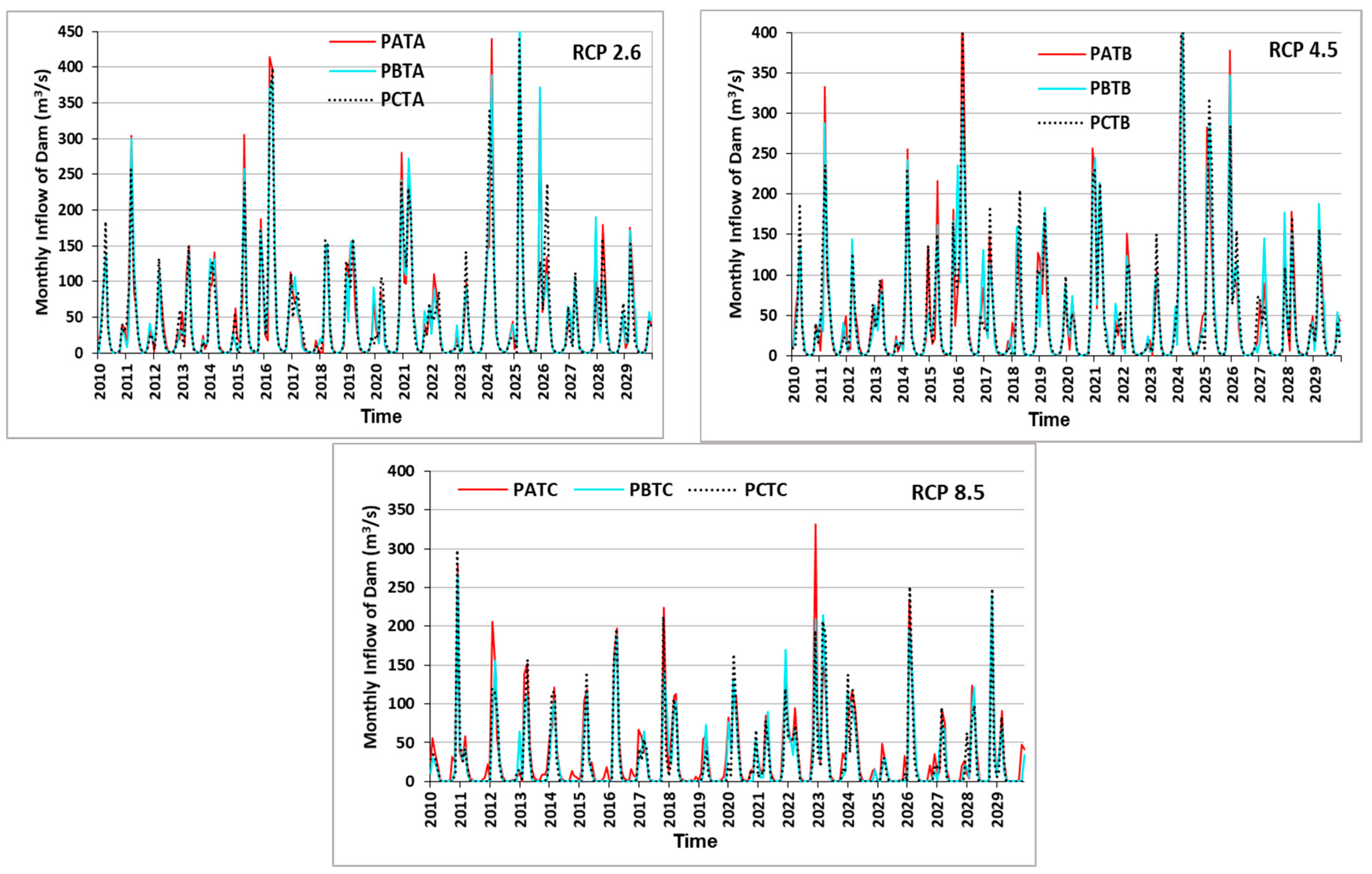
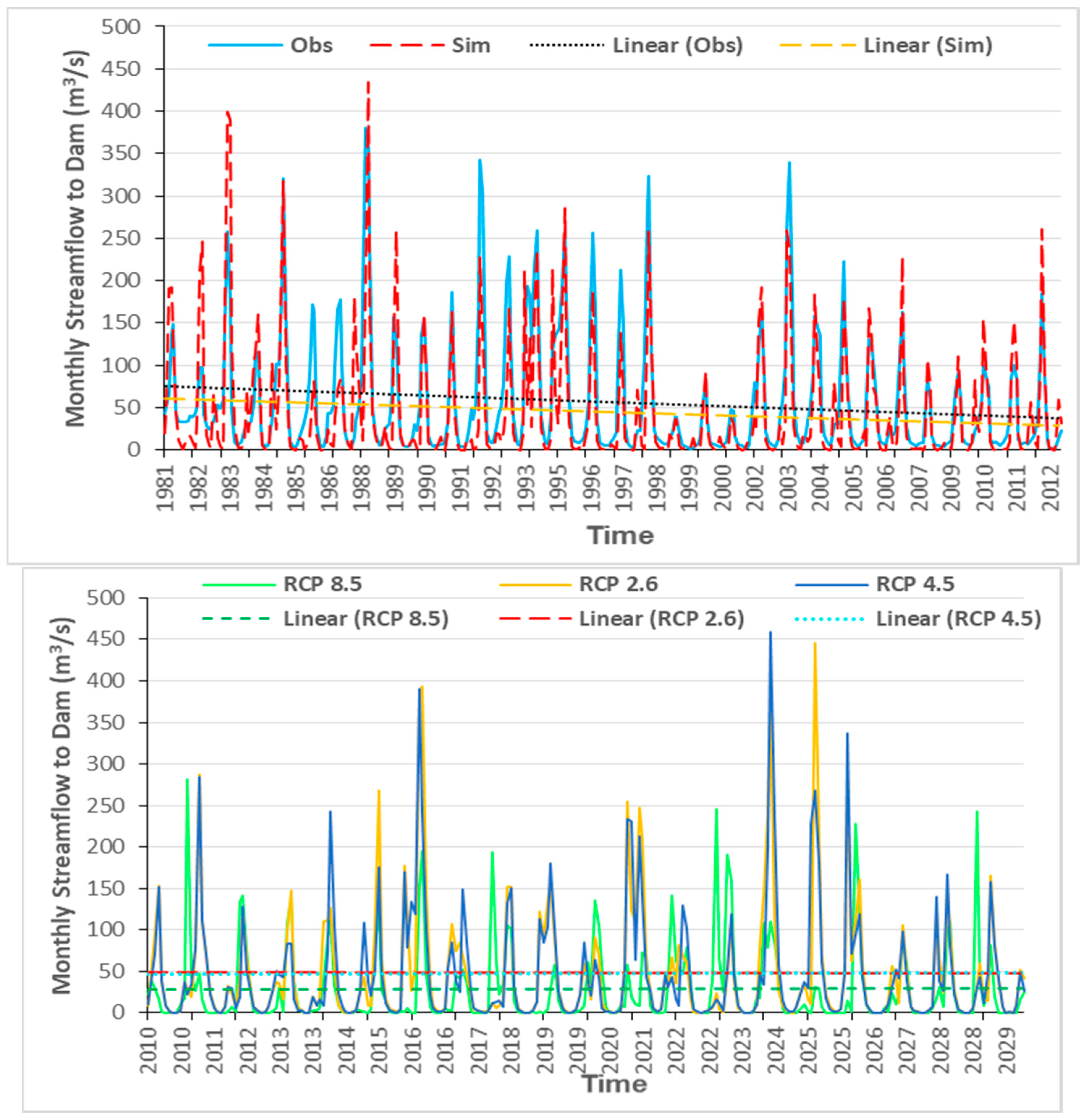
4.5. SWAT Future Dam Inflow Simulations for Various Climate Scenarios
5. Conclusions
Author Contributions
Funding
Conflicts of Interest
References
- Water for Food, Water for Life: A Comprehensive Assessment of Water Management in Agriculture; Earthscan: London, UK; International Water Management Institute: Colombo, Sri Lanka, 2007.
- Voss, K.A.; Famiglietti, J.S.; Lo, M.; Linage, C.D.; Rodell, M.; Swenson, S.C. Groundwater depletion in the Middle East from GRACE with implications for transboundary water management in the Tigris-Euphrates-Western Iran region. Water Resour. Res. 2013, 49, 904–914. [Google Scholar] [CrossRef]
- Madani, K. Water Management in Iran: What is causing the looming crisis? J. Environ. Stud. Sci. 2014, 4, 315–328. [Google Scholar] [CrossRef]
- Punkari, M.; Droogers, P.; Immerzeel, W.; Korhonen, N.; Lutz, A.; Venäläinen, A. Climate Change and Sustainable Water Management in Central Asia; Working Paper Series No. 5; Asian Development Bank (ADB) Central and West Asia: Manila, Philippines, 2014. [Google Scholar]
- Abbaspour, K.C.; Faramarzi, M.; Ghasemi, S.S.; Yang, H. Assessing the Impact of Climate Change on Water Resources of Iran. Water Resour. Res. 2009, 45, W10434. [Google Scholar] [CrossRef]
- Blanc, E.; Strzepek, K.; Schlosser, A.; Jacoby, H.; Gueneau, A.; Fant, C.; Rausch, S.; Reilly, J. Analysis of U.S. Water Resources under Climate Change; MIT Joint Program on the Science and Policy of Global Change, Report No. 239; Massachusetts Institute of Technology: Cambridge, MA, USA, 2013. [Google Scholar]
- Emami, F.; Koch, M. Evaluation of Statistical-Downscaling/Bias-Correction Methods to Predict Hydrologic Responses to Climate Change in the Zarrine River Basin, Iran. Climate 2018, 6, 30. [Google Scholar] [CrossRef]
- Tegegne, G.; Hail, I.D.; Aranganathan, S.M. Evaluation of Operation of Lake Tana Reservoir Future Water Use under Emerging Scenario with and without climate Change Impacts, Upper Blue Nile. Int. J. Comput. Technol. 2013, 4, 654–663. [Google Scholar] [CrossRef]
- Ashraf Vaghefi, S.; Mousavi, S.J.; Abbaspour, K.C.; Srinivasan, R.; Yang, H. Analyses of the impact of climate change on water resources components, drought and wheat yield in semiarid regions: Karkheh River Basin in Iran. Hydrol. Process. 2014, 2018–2032. [Google Scholar] [CrossRef]
- Pengra, B. The Drying of Iran’s Lake Urmia and Its Environmental Consequences; UNEP-GRID; UNEP Global Environmental Alert Service (GEAS): Sioux Falls, SD, USA, 2012. [Google Scholar]
- AghaKouchak, A.; Norouzi, H.; Madani, K.; Mirchi, A.; Azarderakhsh, M.; Nazemi, A.; Nasrollahi, N.; Farahmand, A.; Mehran, A.; Hasanzadeh, E. Aral Sea syndrome desiccates Lake Urmia: Call for action. J. Great Lakes Res. 2015, 41, 307–311. [Google Scholar] [CrossRef]
- Neitsch, S.L.; Arnold, J.G.; Kiniry, J.R.; Williams, J.R. Soil and Water Assessment Tool Theoretical Documentation Version 2009; Texas Water Resources Institute: Temple, TX, USA, 2011. [Google Scholar]
- Jha, M.; Pan, Z.; Takle, E.S.; Gu, R. Impacts of climate change on streamflow in the Upper Mississippi River Basin: A regional climate model perspective. J. Geophys. Res. 2004, 109, D09105. [Google Scholar] [CrossRef]
- Iranian Ministry of Jahade-Agriculture (MOJA). Land Cover Classification; Agricultural Statistics and the Information Center: Tehran, Iran, 2007.
- Ahmadzadeh, H.; Morid, S.; Delavar, M.; Srinivasan, R. Using the SWAT model to assess the impacts of changing irrigation from surface to pressurized systems on water productivity and water saving in the Zarrineh Rud catchment. Agric.Water Manag. 2015. [Google Scholar] [CrossRef]
- Abbaspour, K.C.; Johnson, C.A.; van Genuchten, M.T. Estimating uncertain flow and transport parameters using a sequential uncertainty fitting procedure. J. Vadose Zone 2004, 3, 1340–1352. [Google Scholar] [CrossRef]
- Abbaspour, K.C. SWAT-Calibration and Uncertainty Programs (CUP)—A User Manual; Swiss Federal Institute of Aquatic Science and Technology: Eawag, Duebendorf, 2015. [Google Scholar]
- Koch, M.; Cherie, N. SWAT-Modeling of the Impact of future Climate Change on the Hydrology and the Water Resources in the Upper Blue Nile River Basin, Ethiopia. In Proceedings of the 6th International Conference on Water Resources and Environment Research, ICWRER, Koblenz, Germany, 3–7 June 2013. [Google Scholar]
- Van Griensven, A.; Meixner, T. Dealing with unidentifiable sources of uncertainty within environmental models. In Proceedings of the International Environmental Modelling and Software Society Conference, Osnabrück, Germany, 15–19 June 2014. [Google Scholar]
- Gassman, P.W.; Reyes, M.R.; Green, C.H.; Arnold, J.G. The soil and water assessment tool: Historical development, applications, and future research directions. Trans. ASABE 2007, 50, 1211–1250. [Google Scholar] [CrossRef]
- Krause, P.; Boyle, D.P.; Base, F. Comparison of different efficiency criteria for hydrological model assessment. Adv. Geosci. 2005, 5, 89–97. [Google Scholar] [CrossRef]
- Themeßl, M.J.; Gobiet, A.; Leuprecht, A. Empirical-statistical downscaling and error correction of daily precipitation from regional climate models. Int. J. Climatol. 2011, 31, 1530–1544. [Google Scholar] [CrossRef]
- Emami, F. Development of an algorithm for assessing the impacts of climate change on operation of reservoirs. Master’s Thesis, University of Tehran, Tehran, Iran, 2009. [Google Scholar]
- Sarzaeim, P.; Bozorg-Haddad, O.; Fallah-Mehdipour, E.; Loáiciga, H.A. Climate change outlook for water resources management in a semiarid river basin: The effect of the environmental water demand. Environ. Earth Sci. 2017, 76, 498. [Google Scholar] [CrossRef]
- Van Vuuren, D.P.; Edmonds, J.; Kainuma, M.L.T.; Riahi, K.; Thomson, A.; Matsui, T.; Hurtt, G.; Lamarque, J.F.; Meinshausen, M.; Smith, S.; et al. Representative concentration pathways: An overview. Clim. Chang. 2011, 109. [Google Scholar] [CrossRef]
- Wilby, R.L.; Dawson, C.W.; Barrow, E.M. SDSM—A decision support tool for the assessment of regional climate change impacts. Environ. Model. Softw. 2002, 17, 147–159. [Google Scholar] [CrossRef]
- Wilby, R.L.; Dawson, C.W. Statistical Downscaling Model–Decision Centric (SDSM-DC) Version 5.1 Supplementary Note; Loughborough University: Loughborough, UK, 2013. [Google Scholar]
- Hessami, M.; Gachon, P.; Ouarda, T.B.M.J.; St-Hilaire, A. Automated regression-based statistical downscaling tool. Environ. Model. Softw. 2008, 23, 813–834. [Google Scholar] [CrossRef]
- Themeßl, M.J.; Gobiet, A.; Heinrich, G. Empirical-statistical downscaling and error correction of regional climate models and its impact on the climate change signal. Clim. Chang. 2012, 112, 449–468. [Google Scholar] [CrossRef]
- Miao, C.; Su, L.; Sun, Q.; Duan, Q. A nonstationary bias-correction technique to remove bias in GCM simulations. J. Geophys. Res. Atmos. 2016, 121, 5718–5735. [Google Scholar] [CrossRef]
- Piani, C.; Haerter, J.O.; Coppola, E. Statistical bias correction for daily precipitation in regional climate models over Europe. Theor. Appl. Climatol. 2010, 99, 187–192. [Google Scholar] [CrossRef]
- Li, H.B.; Sheffield, J.; Wood, E.F. Bias correction of monthly precipitation and temperature fields from Intergovernmental Panel on Climate Change AR4 models using equidistant quantile matching. J. Geophys. Res. 2010, 115, D10101. [Google Scholar] [CrossRef]
- Milly, P.C.D.; Betancourt, J.; Falkenmark, M.; Hirsch, R.M.; Kundzewicz, Z.W.; Lettenmaier, D.P.; Stouffer, R.J. Climate change—Stationarity is dead: Whither water management? Science 2008, 319, 573–574. [Google Scholar] [CrossRef]
- Mehran, A.; AghaKouchak, A.; Phillips, T. Evaluation of CMIP5 continental precipitation simulations relative to satellite observations. J. Geophys. Res. Atmos. 2014, 119, 1695–1707. [Google Scholar] [CrossRef]
- Wilks, D.S. Statistical Methods in Atmospheric Sciences, 2nd ed.; Academic Press: Cambridge, MA, USA, 2006. [Google Scholar]
- Mhanna, M.; Bauwens, W. Stochastic single-site generation of daily and monthly rainfall in the Middle East. Meteorol. Appl. 2012, 19, 111–117. [Google Scholar] [CrossRef]
- Arnold, J.G.; Kiniry, J.R.; Sirinivasan, R.; Williams, J.R.; Haney, E.B.; Neitsh, S.L. SWAT Input–Output Documentation, Version 2012; Texas Water Resource Institute: College Station, TX, USA, 2012. [Google Scholar]
- Arnold, J.G.; Moriasi, D.N.; Gassman, P.W.; Abbaspour, K.C.; White, M.J.; Srinivasan, R.; Santhi, C.; Harmel, R.D.; Van Griensven, A.; Van Liew, M.W.; et al. SWAT: Model use, calibration, and validation. Trans. ASABE 2012, 55, 1491–1508. [Google Scholar] [CrossRef]
- Moriasi, D.N.; Arnold, J.G.; Van Liew, M.W.; Bingner, R.L.; Harmel, R.D.; Veith, T.L. Model evaluation guidelines for systematic quantification of accuracy in watershed simulations. Trans. ASABE 2007, 50, 885–900. [Google Scholar] [CrossRef]
- Emami, F.; Koch, M. Agricultural water productivity-based hydro-economic modeling for optimal crop pattern and water resources planning in the zarrine river basin, Iran, in the wake of climate change. Sustainability 2018, 10, 3953. [Google Scholar] [CrossRef]
- Merz, R.; Blöschl, G. A regional analysis of event runoff coefficients with respect to climate and catchment characteristics in Austria. Water Resour. Res. 2009, 45, W01405. [Google Scholar] [CrossRef]
- Emami, F.; Koch, M. Evaluating the water resources and operation of the boukan dam in iran under climate change. Eur. Water 2017, 59, 17–24. [Google Scholar]
- Izady, A.; Davary, K.; Alizadeh, A.; Ziaei, A.N.; Akhavan, S.; Alipoor, A.; Joodavi, A.; Brusseau, M.L. Groundwater conceptualization and modeling using distributed SWAT-based recharge for the semi-arid agricultural Neishaboor plain, Iran. Hydrogeol. J. 2015, 23, 47–68. [Google Scholar] [CrossRef]


| Rank | Parameter | Final Value | Rank | Parameter | Final Value |
|---|---|---|---|---|---|
| 1 | SFTMP.bsn | 1 | 5 | SMFMX.bsn | 7.95 |
| 2 | SMTMP.bsn | 0.5 | 6 | SMFMN.bsn | 0.73 |
| 3 | SNO50COV.bsn | 0.3 | 7 | SNOCOVMX.bsn | 463.9 |
| 4 | TIMP.bsn | 0.71 |
| Rank | Parameter | Dimension | Final Range | Rank | Parameter | Dimension | Final Range |
|---|---|---|---|---|---|---|---|
| 1 | CN2.mgt | dimensionless | 35–89 | 9 | SOL_AWC(1).sol | mm H2O/mm | 0.09–0.34 |
| 2 | SOL_BD(1).sol | g/cm3 | 0.9–1.96 | 10 | ALPHA_BF.gw | 1/day | 0.25–0.96 |
| 3 | SOL_Z(1).sol | mm | 132–476 | 11 | REVAPMN.gw | mm H2O | 162–407 |
| 4 | ALPHA_BNK.rte | days | 0.27–0.65 | 12 | GW_SPYLD.gw * | m3/m3 | 0.05 |
| 5 | GWQMN.gw | mm H2O | 1076–3827 | 13 | CH_K2.rte * | mm/h | 0.5 |
| 6 | ESCO.hru | dimensionless | 0.91–0.99 | 14 | RCHRG_DP.gw * | dimensionless | 0 |
| 7 | SOL_K(1).sol | mm/h | 4–22 | 15 | CH_N2.rte * | dimensionless | 0.016 |
| 8 | GW_DELAY.gw | day | 10–35 |
| Sub-Basin Outlet | Station | Calibration | Validation | ||||||||
|---|---|---|---|---|---|---|---|---|---|---|---|
| P-f * | R-f * | R2 | NS | bR2 | P-f * | R-f * | R2 | NS | bR2 | ||
| 2 | Nezamabad | 0.90 | 1.1 | 0.72 | 0.65 | 0.66 | 0.8 | 1.4 | 0.57 | 0.51 | 0.50 |
| 4 | Chooblooche | 0.82 | 1.0 | .060 | 0.30 | 0.60 | 0.9 | 1.1 | 0.66 | 0.55 | 0.56 |
| 7 | Sarighamish | 0.92 | 1.2 | 0.68 | 0.55 | 0.67 | 0.7 | 1.4 | 0.63 | 0.45 | 0.52 |
| 8 | Boukan Dam | 0.79 | 1.4 | 0.76 | 0.72 | 0.58 | 0.8 | 1.4 | 0.60 | 0.50 | 0.54 |
| 9 | Safakhaneh | 0.85 | 1.1 | 0.66 | 0.40 | 0.62 | 0.8 | 1.2 | 0.59 | 0.45 | 0.55 |
| 11 | Sonateh | 0.86 | 1.1 | 0.64 | 0.42 | 0.63 | 0.6 | 1.7 | 0.55 | 0.44 | 0.30 |
| Average | 0.86 | 1.2 | 0.68 | 0.51 | 0.63 | 0.8 | 1.4 | 0.60 | 0.48 | 0.50 | |
| Parameter | Station Name | R2 | SE | ||
|---|---|---|---|---|---|
| Calibration | Validation | Calibration | Validation | ||
| Min. Temperature | 452255t | 0.66 | 0.74 | 2.03 | 1.65 |
| 453253t | 0.59 | 0.65 | 2.40 | 2.07 | |
| 453254t | 0.63 | 0.69 | 2.18 | 1.78 | |
| 454252t | 0.57 | 0.58 | 2.44 | 2.11 | |
| 454254t | 0.61 | 0.72 | 2.12 | 1.55 | |
| 454255t | 0.65 | 0.76 | 2.03 | 1.60 | |
| 455253t | 0.60 | 0.68 | 2.31 | 1.79 | |
| Max. Temperature | 452255t | 0.71 | 0.79 | 2.01 | 1.81 |
| 453253t | 0.75 | 0.71 | 1.76 | 2.11 | |
| 453254t | 0.73 | 0.81 | 2.05 | 1.65 | |
| 454252t | 0.69 | 0.78 | 2.22 | 1.76 | |
| 454254t | 0.73 | 0.79 | 2.15 | 1.79 | |
| 454255t | 0.71 | 0.79 | 2.12 | 1.80 | |
| 455253t | 0.68 | 0.77 | 2.20 | 1.81 | |
| Average | 0.67 | 0.73 | 2.14 | 1.81 | |
| Percentile | QBt | ||
|---|---|---|---|
| Raw GCM | KDF | ECDF | |
| 25% | 1.48 | 0.69 | 0.96 |
| 50% | 1.35 | 0.57 | 0.87 |
| 75% | 0.86 | 0.46 | 0.79 |
| Average | 1.23 | 0.57 | 0.88 |
| Water Balance Components (mm/a) | Historical Period | RCP 2.6 | RCP 4.5 | RCP 8.5 | |||
|---|---|---|---|---|---|---|---|
| Validation | Calibration | Average | |||||
| Precipitation | 454.6 | 393.1 | 423.9 | 327.2 | 313 | 276 | |
| (−23%) * | (−26%) | (−35%) | |||||
| Snowfall | 145 | 118.3 | 131.7 | 92.8 | 85.6 | 71.36 | |
| (−30%) | (−35%) | (−46%) | |||||
| Sublimation | 38.5 | 38.5 | 38.5 | 32.5 | 27.8 | 24.12 | |
| (−16%) | (−28%) | (−37%) | |||||
| Snowmelt | 105.9 | 79.7 | 92.8 | 65.7 | 58.8 | 49.8 | |
| (−29%) | (−37%) | (−46%) | |||||
| Aquifer Recharge | Shallow | 174.2 | 148.4 | 161.3 | 105.1 | 99.5 | 81.84 |
| (−35%) | (−38%) | (−49%) | |||||
| Deep | 1.4 | 1.1 | 1.3 | 1.1 | 0.7 | 0.72 | |
| (−15%) | (−46%) | (−45%) | |||||
| Evapotranspiration | 254.8 | 253.5 | 254.2 | 197.5 | 209.9 | 162.96 | |
| (−22%) | (−17%) | (−36%) | |||||
| +SWQ | 61.7 | 42.5 | 52.1 | 50.9 | 47.1 | 38.5 | |
| (−2%) | (−10%) | (−26%) | |||||
| +LWQ | 29.7 | 25.2 | 27.5 | 24.9 | 20.5 | 18.16 | |
| (−9%) | (−25%) | (−34%) | |||||
| +GWQ | 133.2 | 101.0 | 117.1 | 87.8 | 69.9 | 63.08 | |
| (−25%) | (−40%) | (−46%) | |||||
| −TLOSS | 2.3 | 1.8 | 2.1 | 1.2 | 1.3 | 1 | |
| (−43%) | (−38%) | (−52%) | |||||
| =WYLD | 222.3 | 166.9 | 194.6 | 162.4 | 136.2 | 119.44 | |
| (−17%) | (−30%) | (−39%) | |||||
| Runoff Coefficient (RC) | 15% | 12% | 14% | 17% | 16% | 15% | |
© 2019 by the authors. Licensee MDPI, Basel, Switzerland. This article is an open access article distributed under the terms and conditions of the Creative Commons Attribution (CC BY) license (http://creativecommons.org/licenses/by/4.0/).
Share and Cite
Emami, F.; Koch, M. Modeling the Impact of Climate Change on Water Availability in the Zarrine River Basin and Inflow to the Boukan Dam, Iran. Climate 2019, 7, 51. https://doi.org/10.3390/cli7040051
Emami F, Koch M. Modeling the Impact of Climate Change on Water Availability in the Zarrine River Basin and Inflow to the Boukan Dam, Iran. Climate. 2019; 7(4):51. https://doi.org/10.3390/cli7040051
Chicago/Turabian StyleEmami, Farzad, and Manfred Koch. 2019. "Modeling the Impact of Climate Change on Water Availability in the Zarrine River Basin and Inflow to the Boukan Dam, Iran" Climate 7, no. 4: 51. https://doi.org/10.3390/cli7040051
APA StyleEmami, F., & Koch, M. (2019). Modeling the Impact of Climate Change on Water Availability in the Zarrine River Basin and Inflow to the Boukan Dam, Iran. Climate, 7(4), 51. https://doi.org/10.3390/cli7040051