Temperature Variability Differs in Urban Agroecosystems across Two Metropolitan Regions


Abstract
1. Introduction
2. Methods
2.1. Study System
2.2. Climate Data and Temperature Measurements
2.2.1. Regional Long-Term Climate Data
2.2.2. Local-Scale Short-Term Weather Data
2.3. Gardener Questionnaires
2.4. Analysis
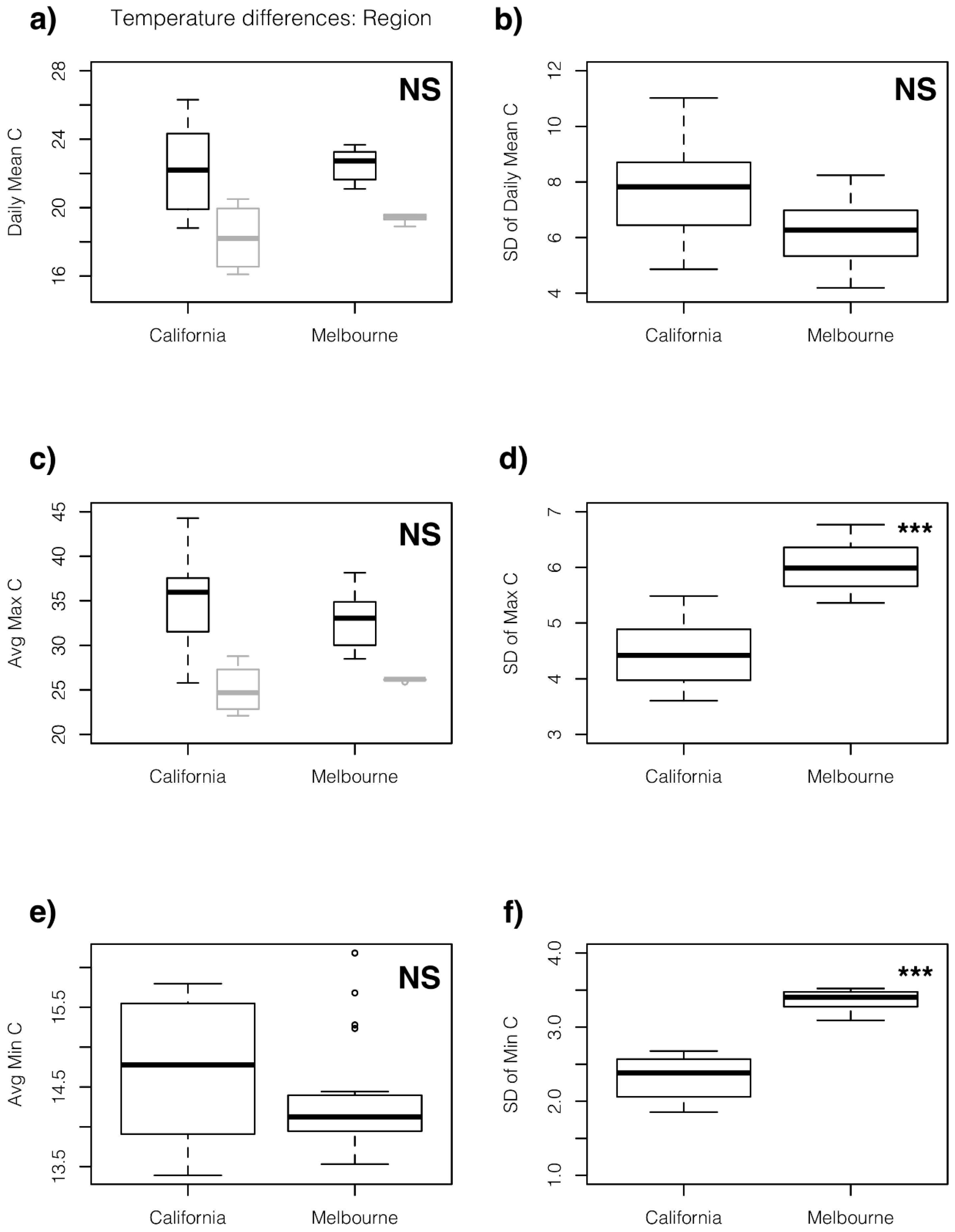
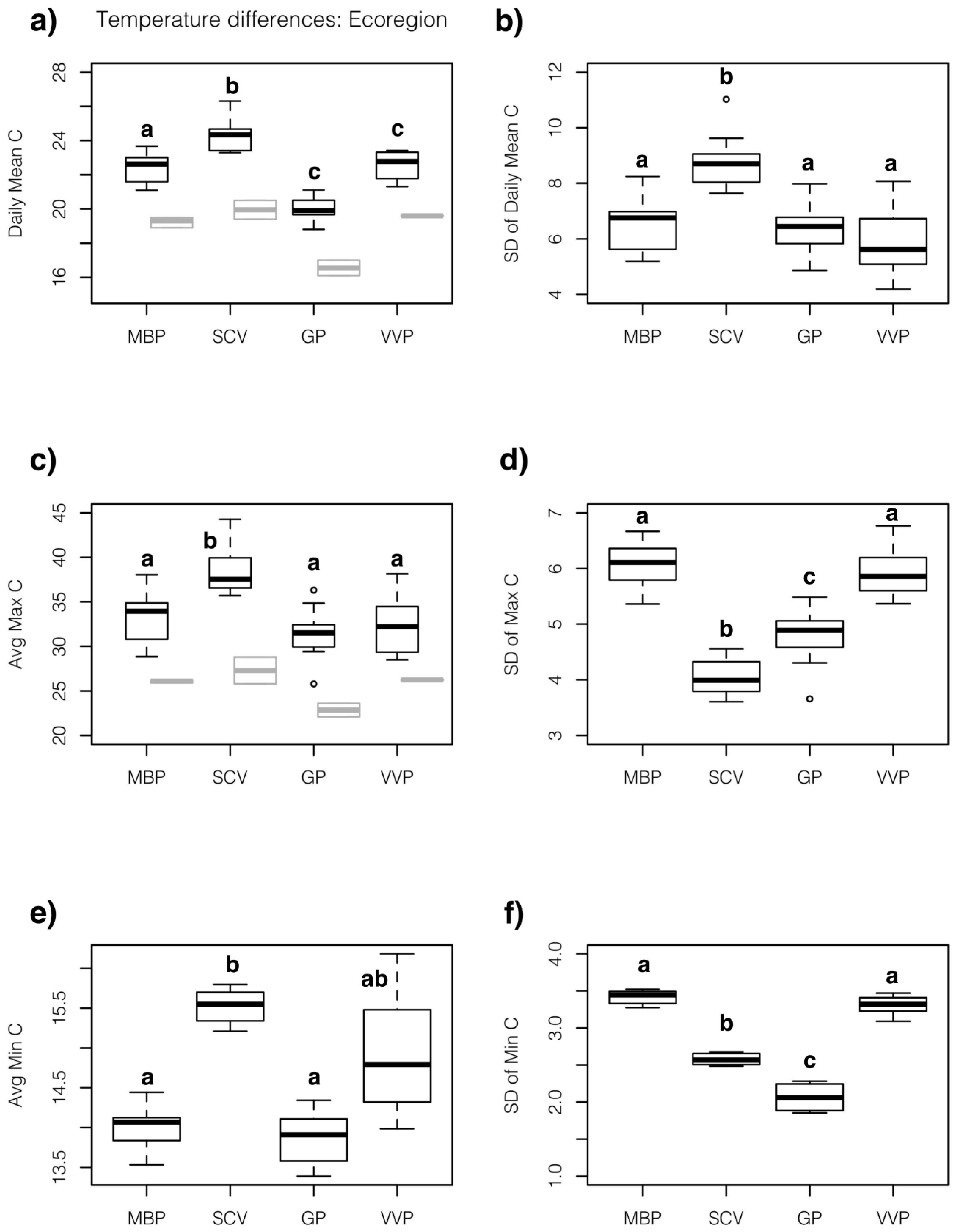
3. Results
3.1. Differences in Long-Term Climate Patterns, and Short-Term Local Temperatures in Gardens across Regions and Ecoregions
3.2. Similarities in Reported Plants Grown by Gardeners
3.3. Climate and Gardeners
4. Discussion
4.1. Relationships between Urban Regional Topography, Agroecosystem Abiotic and Biotic Features, and Environmental Management
4.2. Looking beyond Averages to Examine Variability in Temperatures
4.3. Implications of Temperatures on Human Behavior and Environmental Management
5. Conclusions
Author Contributions
Funding
Acknowledgments
Ethics Approval
Conflicts of Interest
References
- UN-Habitat. World Cities Report 2016: Urbanization and Development: Emerging Futures; United Nations Human Settlements Programme (UN-Habitat): Nairobi, Kenya, 2016; ISBN 9789211333954. [Google Scholar]
- Taha, H. Urban climates and heat islands: Albedo, evapotranspiration, and anthropogenic heat. Energy Build. 1997, 25, 99–103. [Google Scholar] [CrossRef]
- Luber, G.; McGeehin, M. Climate change and extreme heat events. Am. J. Prev. Med. 2008, 35, 429–435. [Google Scholar] [CrossRef]
- Güneralp, B.; Güneralp, İ.; Liu, Y. Changing global patterns of urban exposure to flood and drought hazards. Glob. Environ. Chang. 2015, 31, 217–225. [Google Scholar] [CrossRef]
- Demuzere, M.; Orru, K.; Heidrich, O.; Olazabal, E.; Geneletti, D.; Orru, H.; Bhave, A.G.; Mittal, N.; Feliu, E.; Faehnle, M. Mitigating and adapting to climate change: Multi-functional and multi-scale assessment of green urban infrastructure. J. Environ. Manag. 2014, 146, 107–115. [Google Scholar] [CrossRef] [PubMed]
- Kendal, D.; Williams, N.S.G.; Williams, K.J.H. A cultivated environment: Exploring the global distribution of plants in gardens, parks and streetscapes. Urban Ecosyst. 2012, 15, 637–652. [Google Scholar] [CrossRef]
- City of Melbourne. Urban Forest Strategy: Making a Great City Greener 2012–2032; City of Melbourne: Melbourne, Australia, 2012.
- Tubby, K.V.; Webber, J.F. Pests and diseases threatening urban trees under a changing climate. For. An Int. J. For. Res. 2010, 83, 451–459. [Google Scholar] [CrossRef]
- Kendal, D.; Dobbs, C.; Gallagher, R.V.; Beaumont, L.J.; Baumann, J.; Williams, N.S.G.; Livesley, S.J. A global comparison of the climatic niches of urban and native tree populations. Glob. Ecol. Biogeogr. 2018, 27, 629–637. [Google Scholar] [CrossRef]
- Bowler, D.E.; Buyung-ali, L.; Knight, T.M.; Pullin, A.S. Urban greening to cool towns and cities: A systematic review of the empirical evidence. Landsc. Urban Plan. 2010, 97, 147–155. [Google Scholar] [CrossRef]
- Rosenzweig, C.; Solecki, W.; Hammer, S.A.; Mehrotra, S. Cities lead the way in climate–change action. Nature 2010, 467, 909–911. [Google Scholar] [CrossRef] [PubMed]
- Kong, L.; La Lun-Lau, K.; Yuan, C.; Ren, C.; Ng, E. Regulation of outdoor thermal comfort by trees in Hong Kong. Sustain. Cities Soc. 2017, 31, 12–25. [Google Scholar] [CrossRef]
- Gonçalves, A.; Castro Ribeiro, A.; Maia, F.; Nunes, L.; Feliciano, M. Influence of Green Spaces on Outdoors Thermal Comfort—Structured Experiment in a Mediterranean Climate. Climate 2019, 7, 20. [Google Scholar] [CrossRef]
- Kovats, R.S.; Hajat, S. Heat stress and public health: A critical review. Annu. Rev. Public Health 2008, 29, 41–55. [Google Scholar] [CrossRef] [PubMed]
- Thorsson, S.; Lindqvist, M.; Lindqvist, S. Thermal bioclimatic conditions and patterns of behaviour in an urban park in Goteborg, Sweden. Int. J. Biometeorol. 2004, 48, 149–156. [Google Scholar] [CrossRef]
- Nikolopoulou, M.; Steemers, K. Thermal comfort and psychological adaptation as a guide for designing urban spaces. Energy Build. 2003, 35, 95–101. [Google Scholar] [CrossRef]
- Frumkin, H.; Hess, J.; Luber, G.; Malilay, J.; McGeehin, M. Climate change: The public health response. Am. J. Public Health 2008, 98, 435–455. [Google Scholar] [CrossRef]
- Grothmann, T.; Patt, A. Adaptive capacity and human cognition: The process of individual adaptation to climate change. Glob. Environ. Chang. 2005, 15, 199–213. [Google Scholar] [CrossRef]
- Neil Adger, W.; Arnell, N.W.; Tompkins, E.L. Successful adaptation to climate change across scales. Glob. Environ. Chang. 2005, 15, 77–86. [Google Scholar] [CrossRef]
- Kasperson, R.E.; Renn, O.; Slovic, P.; Brown, H.S.; Emel, J.; Goble, R.; Kasperson, J.X.; Ratick, S. The social amplification of risk: A conceptual framework. Risk Anal. 1988, 8, 177–187. [Google Scholar] [CrossRef]
- Kleerekoper, L.; Van Esch, M.; Salcedo, T.B. How to make a city climate-proof, addressing the urban heat island effect. Resour. Conserv. Recycl. 2012, 64, 30–38. [Google Scholar] [CrossRef]
- Cabral, I.; Costa, S.; Weiland, U.; Bonn, A. Nature-Based Solutions to Climate Change Adaptation in Urban Areas; Springer: Berlin/Heidelberg, Germany, 2017; pp. 237–253. [Google Scholar] [CrossRef]
- Dobbs, C.; Nitschke, C.R.; Kendal, D. Global drivers and tradeoffs of three urban vegetation ecosystem services. PLoS ONE 2014, 9. [Google Scholar] [CrossRef] [PubMed]
- Ossola, A.; Hopton, M.E. Climate differentiates forest structure across a residential macrosystem. Sci. Total Environ. 2018, 639, 1164–1174. [Google Scholar] [CrossRef]
- Stewart, I.D. A systematic review and scientific critique of methodology in modern urban heat island literature. Int. J. Climatol. 2011, 31, 200–217. [Google Scholar] [CrossRef]
- Oke, T.R. Initial Guidance to Obtain Representative Meteorological Observations at Urban Sites. In Instruments and Observing Methods; WHO, Ed.; World Health Organization: Geneva, Switzerland, 2006. [Google Scholar]
- Araos, M.; Austin, S.E.; Berrang-Ford, L.; Ford, J.D. Public health adaptation to climate change in large cities: A global baseline. Int. J. Heal. Serv. 2016, 46, 53–78. [Google Scholar] [CrossRef] [PubMed]
- Hulme, M. Reducing the Future to Climate: A Story of Climate Determinism and Reductionism. Osiris 2011, 26, 245–266. [Google Scholar] [CrossRef]
- WorldClim—Global Climate Data Bioclimatic Variables. Available online: http://www.worldclim.org/bioclim (accessed on 18 December 2018).
- Gill, S.E.; Handley, J.F.; Ennos, A.R.; Pauleit, S. Adapting cities for climate change: The role of green infrastructure. Built. Environ. 2007, 33, 115–133. [Google Scholar] [CrossRef]
- Huang, L.; Li, J.; Zhao, D.; Zhu, J. A fieldwork study on the diurnal changes of urban microclimate in four types of ground cover and urban heat island of Nanjing, China. Build. Environ. 2008, 43, 7–17. [Google Scholar] [CrossRef]
- Lin, B.B.; Egerer, M.H.; Liere, H.; Jha, S.; Bichier, P.; Philpott, S.M. Local- and landscape-scale land cover affects microclimate and water use in urban gardens. Sci. Total Environ. 2018, 610–611, 570–575. [Google Scholar] [CrossRef]
- Egerer, M.H.; Lin, B.B.; Threlfall, C.G.; Kendal, D. Temperature variability influences urban garden plant richness and gardener water use behavior, but not planting decisions. Sci. Total Environ. 2019, 646, 111–120. [Google Scholar] [CrossRef]
- City of Melbourne. City of Melbourne Melbourne Facts and Figures. 2019. Available online: https://www.melbourne.vic.gov.au/about-melbourne/melbourne-profile/Pages/facts-about-melbourne.aspx (accessed on 20 December 2018).
- Bureau of Meteorology Climate Statistics for Australian Locations (Melbourne). Available online: http://www.bom.gov.au/climate/averages/tables/ca_vic_names.shtml (accessed on 15 December 2018).
- Victorian Environmental Assessment. Findings by Bioregion; Victorian Environmental Assessment: Melbourne, Australia, 2010.
- Royal Botanic Gardens Victoria Victorian Volcanic Plain Bioregion. Available online: https://vicflora.rbg.vic.gov.au/flora/bioregions/victorian-volcanic-plain (accessed on 15 December 2018).
- Google Inc Google Earth 2017. Available online: https://earth.google.com/web/ (accessed on 15 January 2019).
- Climate-Data.org Santa Clara Climate: Average Temperature, Weather by Month, Santa Clara Weather Averages. Available online: https://en.climate-data.org/north-america/united-states-of-america/california/santa-clara-1431/ (accessed on 16 December 2018).
- Climate-Data.org Santa Cruz Climate: Average Temperature, Weather by Month, Santa Cruz Weather Averages. Available online: https://en.climate-data.org/north-america/united-states-of-america/california/santa-cruz-6305/ (accessed on 16 December 2018).
- Abdi, H. Coefficient of Variation. In Encyclopedia of Research Design; Salkind, N., Ed.; Sage: Thousand Oaks, CA, USA, 2010; pp. 1–5. [Google Scholar]
- Egerer, M.H.; Lin, B.B.; Philpott, S.M. Water use behavior, learning, and adaptation to future change in urban gardens. Front. Sustain. Food Syst. 2018, 2, 1–14. [Google Scholar] [CrossRef]
- Bolker, B.M.; Brooks, M.E.; Clark, C.J.; Geange, S.W.; Poulsen, J.R.; Stevens, M.H.H.; White, J.-S. Generalized linear mixed models: A practical guide for ecology and evolution. Trends Ecol. Evol. 2009, 24, 127–135. [Google Scholar] [CrossRef]
- Bates, D.; Maechler, M.; Bolker, B.; Walker, S.; Christensen, R.H.B.; Singmann, H. lme4: Linear mixed-effects models using Eigen and S4. R Packag. 2015, 1. Available online: https://cran.r-project.org/web/packages/lme4/ lme4.pdf (accessed on 16 December 2018).
- R Development Core Team R Development Core Team. R: A Language and Environment for Statistical Computing; R Foundation for Statistical Computing: Vienna, Austria, 2016; Volume 55, pp. 275–286. [Google Scholar]
- Fox, J.; Weisberg, S. Companion to applied regression, 2nd ed.; Sage: Thousand Oaks, CA, USA, 2011; Available online: http://socserv.socsci.mcmaster.ca/jfox/ Books/Companion (accessed on 20 December 2018).
- Hothorn, T.; Bretz, F.; Westfall, P. Simultaneous inference in general parametric models. Biom. J. 2008, 50, 346–363. [Google Scholar] [CrossRef]
- McDaniel, M.D.; Tiemann, L.K.; Grandy, A.S. Does agricultural crop diversity enhance soil microbial biomass and organic matter dynamics? A meta-analysis. Ecol. Appl. 2014, 24, 560–570. [Google Scholar] [CrossRef]
- Lin, B.B.; Flynn, D.F.B.; Bunker, D.E.; Uriarte, M. The effect of agricultural diversity and crop choice on functional capacity change in grassland conversions. J. Appl. Ecol. 2011, 609–618. [Google Scholar] [CrossRef]
- Hijmans, R.J.; Cameron, S.E.; Parra, J.L.; Jones, P.G.; Jarvis, A. Very high resolution interpolated climate surfaces for global land areas. Int. J. Climatol. 2005, 25, 1965–1978. [Google Scholar] [CrossRef]
- Watkins, R.; Palmer, J.; Kolokotroni, M. Increased temperature and intensification of the Urban Heat Island: Implications for human comfort and urban design. Built Environ. 2007, 33, 85–96. [Google Scholar] [CrossRef]
- Stone, B.; Hess, J.J.; Frumkin, H. Urban form and extreme heat events: Are sprawling cities more vulnerable to climate change than compact cities? Environ. Health Perspect. 2010, 118, 1425–1428. [Google Scholar] [CrossRef]
- Teixeira, E.I.; Fischer, G.; van Velthuizen, H.; Walter, C.; Ewert, F. Global hot-spots of heat stress on agricultural crops due to climate change. Agric. For. Meteorol. 2013, 170, 206–215. [Google Scholar] [CrossRef]
- Barlow, K.M.; Christy, B.P.; O’Leary, G.J.; Riffkin, P.A.; Nuttall, J.G. Simulating the impact of extreme heat and frost events on wheat crop production: A review. Field Crop. Res. 2015, 171, 109–119. [Google Scholar] [CrossRef]
- Battisti, D.S.; Naylor, R.L. Historical Warnings of Future Food Insecurity with Unprecedented Seasonal Heat. Science 2009, 323, 240–244. [Google Scholar] [CrossRef] [PubMed]
- Armson, D.; Stringer, P.; Ennos, A.R. The effect of tree shade and grass on surface and globe temperatures in an urban area. Urban For. Urban Green. 2012, 11, 245–255. [Google Scholar] [CrossRef]
- Gourdji, S.M.; Sibley, A.M.; Lobell, D.B. Global crop exposure to critical high temperatures in the reproductive period: Historical trends and future projections. Environ. Res. Lett. 2013, 8. [Google Scholar] [CrossRef]
- Lobell, D.B.; Schlenker, W.; Costa-Roberts, J. Climate trends and global crop production since 1980. Science 2011, 333, 616–620. [Google Scholar] [CrossRef] [PubMed]
- Klein, R.J.T.; Nicholls, R.J.; Mimura, N. Coastal adaptation to climate change: Can the IPCC Technical Guidelines be applied? Mitig. Adapt. Strateg. Glob. Chang. 1999, 4, 239–252. [Google Scholar] [CrossRef]
- Lin, B.B.; Egerer, M.H.; Ossola, A. Urban gardens as a space to engender biophilia: Evidence and ways forward. Front. Built Environ. 2018, 4, 1–10. [Google Scholar] [CrossRef]


| Region | Ecoregion | Avg. Annual Mean Temp. (°C) | Avg. Mean Temp. of Warmest Quarter (°C) | Avg. Mean Temp. of Coldest Quarter (°C) | Avg. of Annual Precipitation (mm) |
|---|---|---|---|---|---|
| Central Coast, California | 14.35 | 18.25 | 10.23 | 481.50 | |
| Santa Clara Valley | 15.15 | 19.95 | 10.05 | 412.00 | |
| Monterey Bay Plains | 13.55 | 16.55 | 10.40 | 551.00 | |
| Melbourne, Victoria | 14.58 | 19.36 | 9.76 | 757.60 | |
| Gippsland Plain | 14.43 | 19.20 | 9.63 | 827.67 | |
| Victorian Volcanic Plain | 14.80 | 19.60 | 9.95 | 652.50 |
| Models | Explanatory Variables (Local-Scale Temperature Data in Gardens) |
|---|---|
| (a) Between regions: California vs. Melbourne, Victoria | Average temperature |
| (b) Between ecoregions | Temperature variability SD |
| Average maximum temperature | |
| Maximum temperature SD | |
| Average minimum temperature | |
| Minimum temperature SD |
| Model | Coefficient | SE | DF | t | p | AIC | |||
|---|---|---|---|---|---|---|---|---|---|
| a) | Mean Temp | ~ | Intercept | 22.18 | 0.83 | 31 | 26.67 | <0.001 | 128.46 |
| Region (M) | 0.30 | 1.12 | 7 | 0.26 | 0.80 | ||||
| Mean Temp | ~ | Intercept (M-GP) | 22.41 | 0.28 | 31 | 80.69 | <0.001 | 112.02 | |
| CA-SCV b | 1.90 | 0.42 | 5 | 4.52 | 0.006 | ||||
| CA-MBP c | −2.37 | 0.42 | 5 | −5.64 | 0.002 | ||||
| M-VVP a | 0.15 | 0.44 | 5 | 0.33 | 0.75 | ||||
| b) | SD of Temp | ~ | Intercept | 7.61 | 0.52 | 31 | 14.73 | <0.001 | 134.72 |
| Region (M) | −1.33 | 0.70 | 7 | −1.90 | 0.10 | ||||
| SD of Temp | ~ | Intercept (M-GP) | 6.54 | 0.34 | 31 | 19.37 | <0.001 | 127.01 | |
| CA-SCV b | 2.23 | 0.51 | 5 | 4.36 | 0.007 | ||||
| CA-MBP a | −0.08 | 0.51 | 5 | −0.16 | 0.88 | ||||
| M-VVP a | −0.65 | 0.53 | 5 | −1.21 | 0.28 | ||||
| c) | Avg Max C | ~ | Intercept | 35.04 | 1.50 | 31 | 23.41 | <0.001 | 215.74 |
| Region (M) | −2.16 | 2.03 | 7 | −1.07 | 0.32 | ||||
| Avg Max C | ~ | Intercept (M-GP) | 33.24 | 0.89 | 31 | 37.35 | <0.001 | 202.69 | |
| CA-SCV b | 5.34 | 1.33 | 5 | 4.01 | 0.01 | ||||
| CA-MBP a | −1.74 | 1.33 | 5 | −1.31 | 0.25 | ||||
| M-VVP a | −0.91 | 1.41 | 5 | −0.65 | 0.55 | ||||
| d) | SD of Max C | ~ | Intercept | 4.44 | 0.16 | 31 | 27.78 | <0.001 | 67.60 |
| Region (M) | 1.57 | 0.22 | 7 | 7.17 | <0.001 | ||||
| SD of Max C | ~ | Intercept (M-GP) | 6.06 | 0.13 | 31 | 48.37 | <0.001 | 65.19 | |
| CA-SCV b | −1.98 | 0.19 | 5 | −10.65 | <0.001 | ||||
| CA-MBP c | −1.26 | 0.19 | 5 | −6.79 | 0.001 | ||||
| M-VVP a | −0.13 | 0.20 | 5 | −0.64 | 0.55 | ||||
| e) | Avg Min. C | ~ | Intercept | 14.69 | 0.42 | 31 | 35.16 | <0.001 | 38.78 |
| Region (M) | −0.33 | 0.56 | 7 | −0.58 | 0.58 | ||||
| Avg Min. C | ~ | Intercept (M-GP) | 14.00 | 0.28 | 31 | 50.19 | <0.001 | 32.51 | |
| CA-SCV b | 1.52 | 0.44 | 5 | 3.46 | 0.02 | ||||
| CA-MBP a | −0.13 | 0.44 | 5 | −0.29 | 0.78 | ||||
| M-VVP ab | 0.92 | 0.44 | 5 | 2.09 | 0.09 | ||||
| f) | SD of Min C | ~ | Intercept | 2.32 | 0.12 | 31 | 20.05 | <0.001 | −52.87 |
| Region (M) | 1.05 | 0.16 | 7 | 6.77 | <0.001 | ||||
| SD of Min C | ~ | Intercept (M-GP) | 3.42 | 0.08 | 31 | 41.97 | <0.001 | −53.52 | |
| CA-SCV b | −0.84 | 0.13 | 5 | −6.55 | 0.001 | ||||
| CA-MBP c | −1.35 | 0.13 | 5 | −10.54 | <0.001 | ||||
| M-VVP a | −0.11 | 0.13 | 5 | −0.85 | 0.43 |
| Theme | Surveyed Gardeners in the Central Coast, California | Surveyed Gardeners in Melbourne, Victoria |
|---|---|---|
| Climate change | Perceived drought:
| Perceived drought, extreme heat, and unpredictability:
|
| Effects on garden | Perceived water availability in the garden:
| Perceived effects on garden plants:
|
| Effects on gardening practice | Reported effects on watering behavior (e.g., timing, amount used):
| Reported effects on watering behavior (e.g., timing, amount used) and plant selection:
|
© 2019 by the authors. Licensee MDPI, Basel, Switzerland. This article is an open access article distributed under the terms and conditions of the Creative Commons Attribution (CC BY) license (http://creativecommons.org/licenses/by/4.0/).
Share and Cite
Egerer, M.H.; Lin, B.B.; Kendal, D. Temperature Variability Differs in Urban Agroecosystems across Two Metropolitan Regions. Climate 2019, 7, 50. https://doi.org/10.3390/cli7040050
Egerer MH, Lin BB, Kendal D. Temperature Variability Differs in Urban Agroecosystems across Two Metropolitan Regions. Climate. 2019; 7(4):50. https://doi.org/10.3390/cli7040050
Chicago/Turabian StyleEgerer, Monika H., Brenda B. Lin, and Dave Kendal. 2019. "Temperature Variability Differs in Urban Agroecosystems across Two Metropolitan Regions" Climate 7, no. 4: 50. https://doi.org/10.3390/cli7040050
APA StyleEgerer, M. H., Lin, B. B., & Kendal, D. (2019). Temperature Variability Differs in Urban Agroecosystems across Two Metropolitan Regions. Climate, 7(4), 50. https://doi.org/10.3390/cli7040050