A Lagrangian Ocean Model for Climate Studies

Department of Geology and Geophysics, Yale University, New Haven, CT 06511, USA
Climate 2019, 7(3), 41; https://doi.org/10.3390/cli7030041
Submission received: 1 February 2019
/
Revised: 7 March 2019
/
Accepted: 9 March 2019
/
Published: 15 March 2019
(This article belongs to the Special Issue Climate and Atmospheric Dynamics and Predictability)
Abstract
Most weather and climate models simulate circulations by numerically approximating a complex system of partial differential equations that describe fluid flow. These models also typically use one of a few standard methods to parameterize the effects of smaller-scale circulations such as convective plumes. This paper discusses the continued development of a radically different modeling approach. Rather than solving partial differential equations, the author’s Lagrangian models predict the motions of individual fluid parcels using ordinary differential equations. They also use a unique convective parameterization, in which the vertical positions of fluid parcels are rearranged to remove convective instability. Previously, a global atmospheric model and basin-scale ocean models were developed with this approach. In the present study, components of these models are combined to create a new global Lagrangian ocean model (GLOM), which will soon be coupled to a Lagrangian atmospheric model. The first simulations conducted with the GLOM examine the contribution of interior tracer mixing to ocean circulation, stratification, and water mass distributions, and they highlight several special model capabilities: (1) simulating ocean circulations without numerical diffusion of tracers; (2) modeling deep convective transports at low resolution; and (3) identifying the formation location of ocean water masses and water pathways.
1. Introduction
Many aspects of geophysical fluid dynamics are most easily modeled in a frame of reference that moves along with the fluid. For example, we show below that in such a framework three relatively simple ordinary differential equations predict large-scale fluid motions and local changes to fluid tracers (Section 2.3). While partially Lagrangian models, in which fluid particles are tracked in flow fields simulated by Eulerian methods, are becoming increasingly popular for both the atmosphere and the oceans [1,2,3], few fully Lagrangian general circulation models have been used for either the oceans or the atmosphere. This paper discusses the development of a fully Lagrangian model for simulating global ocean circulations.
One particular application the author has in mind for this model, is to couple it to his fully Lagrangian atmospheric model (LAM) [4]. The resulting Lagrangian coupled model is expected to be useful for weather and climate prediction as well as climate dynamics experiments. The LAM has already had success in simulating the Madden Julian Oscillation (MJO) [4,5,6], a planetary scale tropical weather disturbance [7] that is poorly represented in many atmospheric models [8,9,10], and which has global impacts on weather and climate [11,12,13]. The MJO also represents a component of the global atmospheric circulation that is predictable at much longer time scales than mid-latitude baroclinic waves [14]. The LAM has a unique spherical geometry [4], which as we note below is shared by the new global Lagrangian ocean model (GLOM), which makes the GLOM well suited for coupling to the LAM. However, there are many other potential advantages and applications for a fully Lagrangian global ocean model.
One such advantage is that the GLOM can circulate water without producing numerical tracer diffusion. A tracer value for a given water parcel does not change unless a tracer source is included, or a parameterization of tracer mixing is applied [15]. This contrasts with the behavior of z-coordinate ocean models, which generate an uncertain amount of spurious numerical mixing associated with the advection of tracers [16]. While isopycnal models [17] remove spurious numerical mixing of tracers across isopycnal surfaces—essentially by using a Lagrangian vertical coordinate—they also generate numerical mixing of tracers in modeling flow along isopycnals.
Another advantage of Lagrangian modeling relevant to this study relates to the parameterization of convection. In nature, when a fluid is unstable, convective plumes form that transport dense fluid downward and less dense fluid upward. The horizontal scale of the convective circulations is typically much smaller than that of the grid spacing for a large-scale model. What geophysical convective plumes ultimately accomplish is transporting fluid to a different layer. For example, in the atmosphere, tropical deep convection moves air from the boundary layer to the upper troposphere [18], and mid-level air to the boundary layer [19]. In the ocean, deep convective plumes move dense water from near the surface to the ocean bottom. As noted in Section 2.2, the Lagrangian convective parameterization produces the same vertical transport—by changing the vertical positioning of parcels—without attempting to model the details of the small-scale circulation in the convective plumes. The author believes that this unique convective parameterization has helped the LAM to simulate MJOs with realistic vertical structures and life cycles [4,5,6].
A third advantage of the Lagrangian approach to weather and climate modeling is that it provides fluid trajectory information for every mass element in the oceans and the atmosphere. Each component of fluid mass has an identification number that does not change during the course of a simulation [4,15]. The modeler can look up the position of a given mass element at all previous times for which model data is saved with no additional computations. It is hard to overemphasize the utility of this information. For example, it is well known that in the ocean, water mass characteristics are intimately connected to the locations in which they form, which is why water masses are given names like “North Atlantic Deep Water”, “Antarctic Bottom Water”, and “Antarctic Intermediate Water”. The Lagrangian ocean modeler can easily determine where each water parcel last had contact with the surface (e.g., see Section 3.5). Similarly, in the atmosphere, the air temperature and moisture of a given air parcel are strongly dependent on previous locations of the parcel, with terms like “Artic Air” or “Gulf Moisture” (indicated moisture coming from the Gulf of Mexico) frequently used by meteorologists, and transports of moisture largely determining where moist convective systems form and move [4].
Finally, we note that perhaps the most important benefit of developing fully Lagrangian weather and climate modeling components, is that they will increase the genetic diversity of models. By perturbating the planet’s radiative forcing, humans are essentially using the earth as a laboratory for a giant climate experiment with unknown consequences. We need a diversity of tools to map out the possible impacts of this experiment. Much in the same way that different kinds of engines (e.g., standard combustion, diesel, electric motors) have different niches for which they are best suited, so it is for different kinds of models of the atmosphere and oceans. The models and parameterizations that are the most fundamentally different from the others make the largest contribution to diversity. The Lagrangian tools presented here fit into that category. Much in the same way that the unique animals living in Australia are a great treasure to the biologist, Lagrangian modeling components are unique, and they have the potential to provide a fresh and fundamentally different perspective on ocean and atmosphere modeling and dynamics.
The work presented in this paper builds on a number of previous studies involving Lagrangian models of lakes and oceans. Haertel and Randall [20] developed a Lagrangian numerical method for the oceans in which a body of water was represented as a collection of conforming water parcels referred to as “slippery sacks”. This method was closely related to two Lagrangian numerical methods used at that time: partical in cell (PIC; [21]) and smoothed particle hydrodynamics (SPH; [22]). However, in geophysical applications, PIC had only been used for one or two layers of fluid (e.g., [23]), and the slippery sacks method differed from SPH in that two conforming water parcels could not occupy the same physical space whereas two SPH particles could. Consequently, as slippery sacks moved around, they maintained a fairly uniform distribution over time, whereas regions highly concentrated with particles or nearly void of particles could develop under SPH. Haertel et al. [24] adapted horizontal and vertical mixing schemes to the slippery sacks method and created a three-dimensional model of a large lake. Haertel et al. [25] developed an idealized Lagrangian model of the North Atlantic Ocean. Haertel and Fedorov [15] added an Antarctic circumpolar to the idealized Atlantic Ocean Model. Applications of these models have included large lake upwelling [24], simulation of Stommel and Munk solutions [25], modeling of the circulation and stratification in the North Atlantic Ocean [15,25,26], and simulations of idealized equatorial oceans and tropical instability waves [27].
This study advances our previous Lagrangian ocean modeling efforts in several ways. In particular, for the first time global spherical geometry and realistic bottom topography are included in an ocean model. This means that for the first time a fully Lagrangian ocean general circulation model is presented that can be used in global weather and climate modeling and climate dynamics experiments. This model (the GLOM) was developed by combining components of the Lagrangian basin-scale ocean model used by Haertel and Fedorov [15] and the Lagrangian atmospheric model developed by Haertel et al. [4] This paper presents the first simulations conducted with the GLOM, which not only provide evidence of its usefulness as a climate modeling tool, but also help to illustrate the role of interior tracer mixing in maintaining global ocean circulation and stratification. This paper is organized as follows. Section 2 describes the components of the GLOM. Section 3 presents our first fully Lagrangian simulations of global oceans. Section 4 discusses the results presented in light of other studies.
2. Materials and Methods
The primary data source for this study is the Global Lagrangian Ocean Model (GLOM). It was developed by combining components of several previous Lagrangian ocean and atmosphere models. Each of these model components is briefly described in this section with the goal of providing the reader with an intuitive understanding of how they work. More complete technical details are available from the original references that discuss the development of particular model components.
2.1. Fluid Parcels
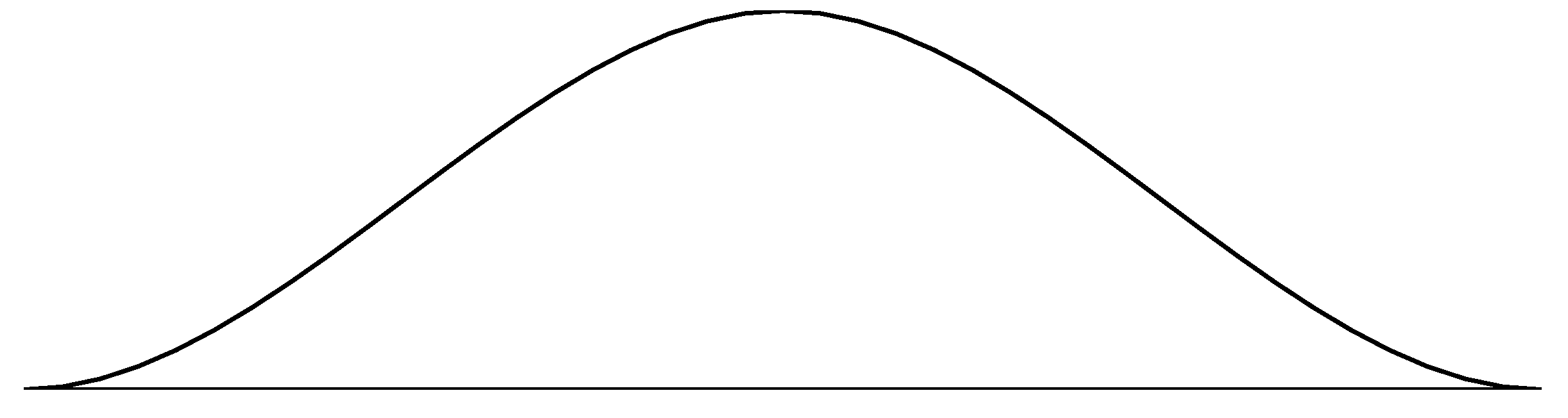
The GLOM represents a body of water as a collection of flexible water parcels [20]. Each parcel has a horizontal mass distribution function that remains fixed in the parcel’s frame of reference (Figure 1).
The mass distribution function defines the amount of mass per unit of horizontal area between the top and bottom surface of the parcel. Since density variations in the ocean are small, this function also provides a good approximation of the shape of the vertical thickness of a parcel, and it is also referred to as the “vertical thickness” function. Here, we use a third-order polynomial in each horizontal dimension (latitude and longitude) to define the mass distribution function following [24]. Constructing the mass distribution function in this manner is computationally efficient, and it helps with conserving energy when calculating the pressure force, which also guarantees numerical stability [20]. Although this means that the horizontal projection of a parcel is a square, it turns out that most of the contours of vertical thickness are circular, as is illustrated in Figure 2b of [27].
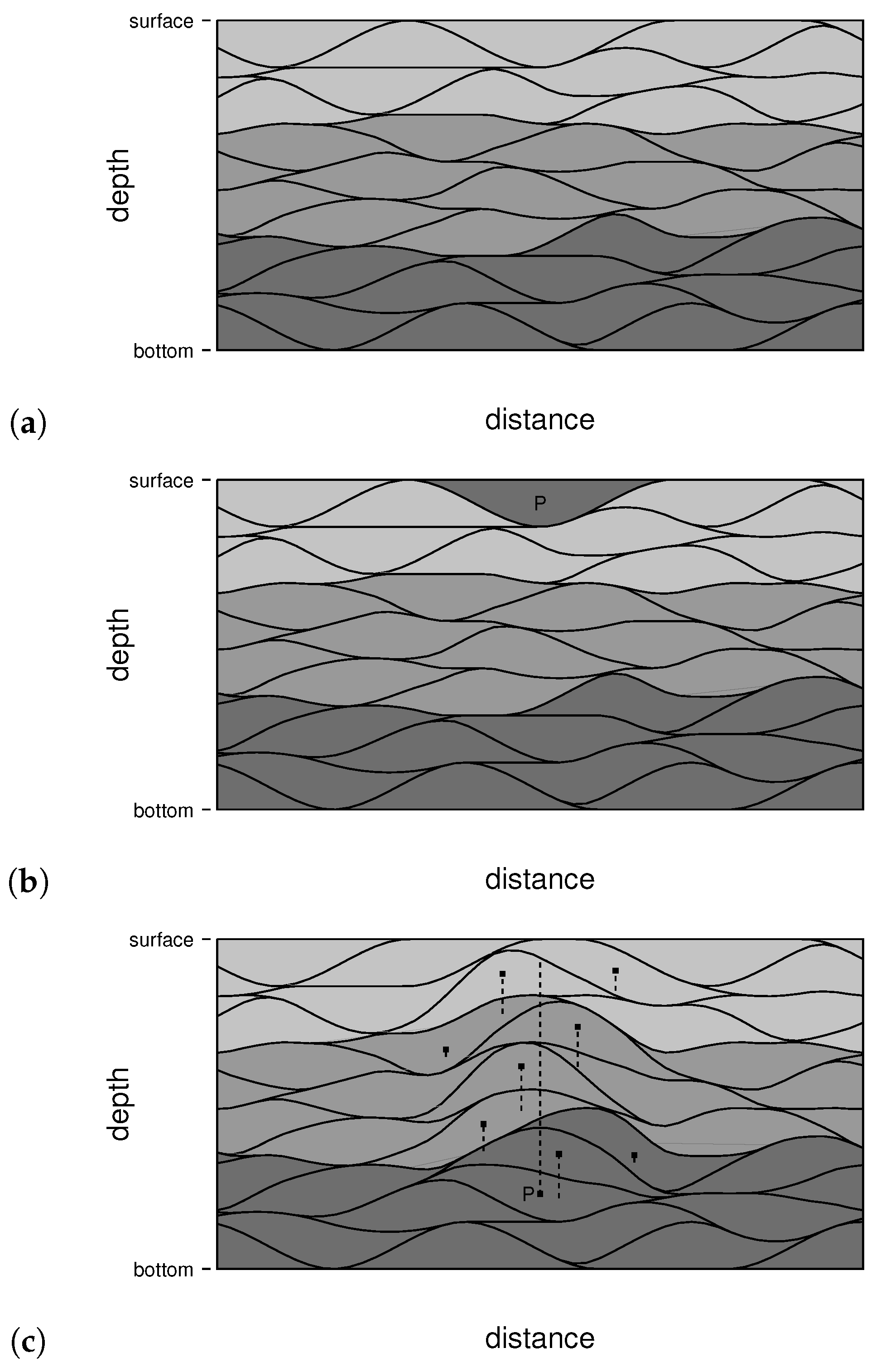
Each column of mass within a given parcel can move up or down independently of neighboring columns as the parcel slides over variable bottom topography or other parcels. So, although all parcels have the same horizontal mass distribution or vertical thickness function (Figure 1), parcels have a variety of shapes owing to vertical shearing (e.g., Figure 2a). As parcels slide over one another, they conform, so there are no gaps between parcels. Since each parcel has a fixed amount of mass associated with it, parcel centers maintain an approximately uniform distribution. When two parcels meet, the parcel with a greater density slides under the parcel with a lesser density, so the fluid maintains a neutral or stable stratification (Figure 2a; note that darker shading denotes denser parcels).
2.2. Lagrangian Convective Parameterization
On occasion, cooling or an increase in salinity can cause a near surface parcel to become more dense than parcels beneath it (Figure 2b). The Lagrangian convective parameterization then changes the stacking order of the parcels, so a neutral or stable stratification is restored (Figure 2c). Note that as the dense parcel sinks, neighboring parcels rise around it (Figure 2c; dashes lines denote vertical displacements of individual parcel centers). In this study, there is no mixing between convective updrafts and downdrafts (i.e., rising and sinking parcels). In atmospheric applications, we have found that carefully setting convective mixing (i.e., entrainment) is a key to accurately simulating moist convective systems such as the Madden Julian Oscillation [4,5,6].
Note that Figure 2 is a schematic illustration of the Lagrangian convective scheme, and it is intended to provide the reader with a mental picture, or intuitive understanding of how the parameterization works. For simplicity, the parcels have been drawn in two dimensions in an extremely coarse-resolution box-shaped ocean. A depiction of parcel interfaces for the simulations in this paper would include many more lines, a varying free surface elevation, and irregular bottom topography. Moreover, the GLOM does not actually keep track of parcel interfaces, but only the positions of parcel centers. The horizontal position vector for each parcel is a prognostic model variable (see below), whereas the vertical position of a given parcel depends on the vertical thicknesses of parcels beneath it. Near the beginning of each model time step, the vertical positions are diagnosed one parcel at a time starting with the lowest (most dense) parcel. The way that the convective scheme is implemented in the model is parcels are sorted by density after each time step, so density is a non-increasing function of the parcel array index, which determines the stacking order.
There are several limitations to this convective scheme. First, it is primarily intended to represent the net transports by deep, buoyancy-driven convection. The depth to which a parcel sinks is determined by its density relative to that of the environment (Figure 2). It is not intended to represent near-surface wind driven convection due to turbulent mixing, which can determine the depth of the surface boundary layer. Moreover, this scheme does not predict convective vertical velocities or accelerations of parcels, but rather the integrated effects of transports by updrafts and downdrafts. While mixing between rising and sinking parcels (i.e., entrainment) has been implemented and tested in atmospheric applications, it has not yet been tested in ocean simulations.
2.3. Model Equations
The following equations describe the motions of a fluid parcel:
where x is horizontal position, u is horizontal velocity, f is the Coriolis parameter, Ap is the acceleration due to pressure, and Am is the acceleration resulting from the mixing of momentum (i.e., viscosity). Evaluating the pressure acceleration involves approximating an integral of pressure over the surface of a parcel with a Riemann sum. Haertel et al. [24] developed a method to efficiently evaluate this sum for every parcel, and for technical details the reader is referred to that study. The pressure force is then divided by the parcel mass to yield the pressure acceleration vector. Vertical motion occurs when a parcel slides up or down variable topography, and/or when there is mass convergence or divergence beneath a parcel (i.e., as in conventional hydrostatic fluid models).
A fluid tracer q changes only in response to sources and mixing:
where Sq is the source of the tracer and Mq denotes mixing. In this study, the only tracer we consider is temperature, because we use the following simple equation of state:
where is density, and T is temperature. The only temperature source for parcels is in the surface layer, where a restoring temperature is applied (see Section 2.7). The author chose not to include salinity’s effects on density for several reasons. First, he judged the transition from basin-scale ocean simulations with idealized topography to global-scale simulations with realistic topography, along with the required rewrite of much of the model code, to be a task of sufficient complexity in and of itself without using a new equation of state. Second, a major goal of this paper is to extend the results of [15] to global scales and they did not use an equation of state with salinity. Third, the author’s next planned application for the GLOM involves studying the impacts of air–sea coupling on the dynamics of the Madden Julian Oscillation, which does not require the use of an equation of state with salinity variations. In nature, of course, salinity variations make important contributions to density, so in interpreting the simulations presented here and comparing to observed ocean structure, it is probably best to think of temperature as a proxy for density.
2.4. Mixing
For the purposes of computing horizontal and vertical mixing, the domain is divided into isopycnal layers and columns respectively [24,25]. Columns of points are treated like columns of points in a finite difference model following [24]. Within isopycnal layers, parcels are allowed to mix momentum with their nearest neighbors following [25]. The Gent Mcwilliams [28] parameterization of mixing by eddies is not explicitly included, but Haertel and Fedorov [15] found that random motions of parcels generate a similar kind of mixing in this kind of Lagrangian model. The vertical viscosity is set to 10 cm2 s−1, and the horizontal viscosity is set to 3 × 10⁴ m2 s−1. For the simulation with interior mixing, the vertical tracer diffusivity is 1 cm2 s−1 (it is zero in the simulation without interior mixing). The horizontal tracer diffusivity is set to zero for both simulations.
2.5. Bottom Topography and Spherical Geometry
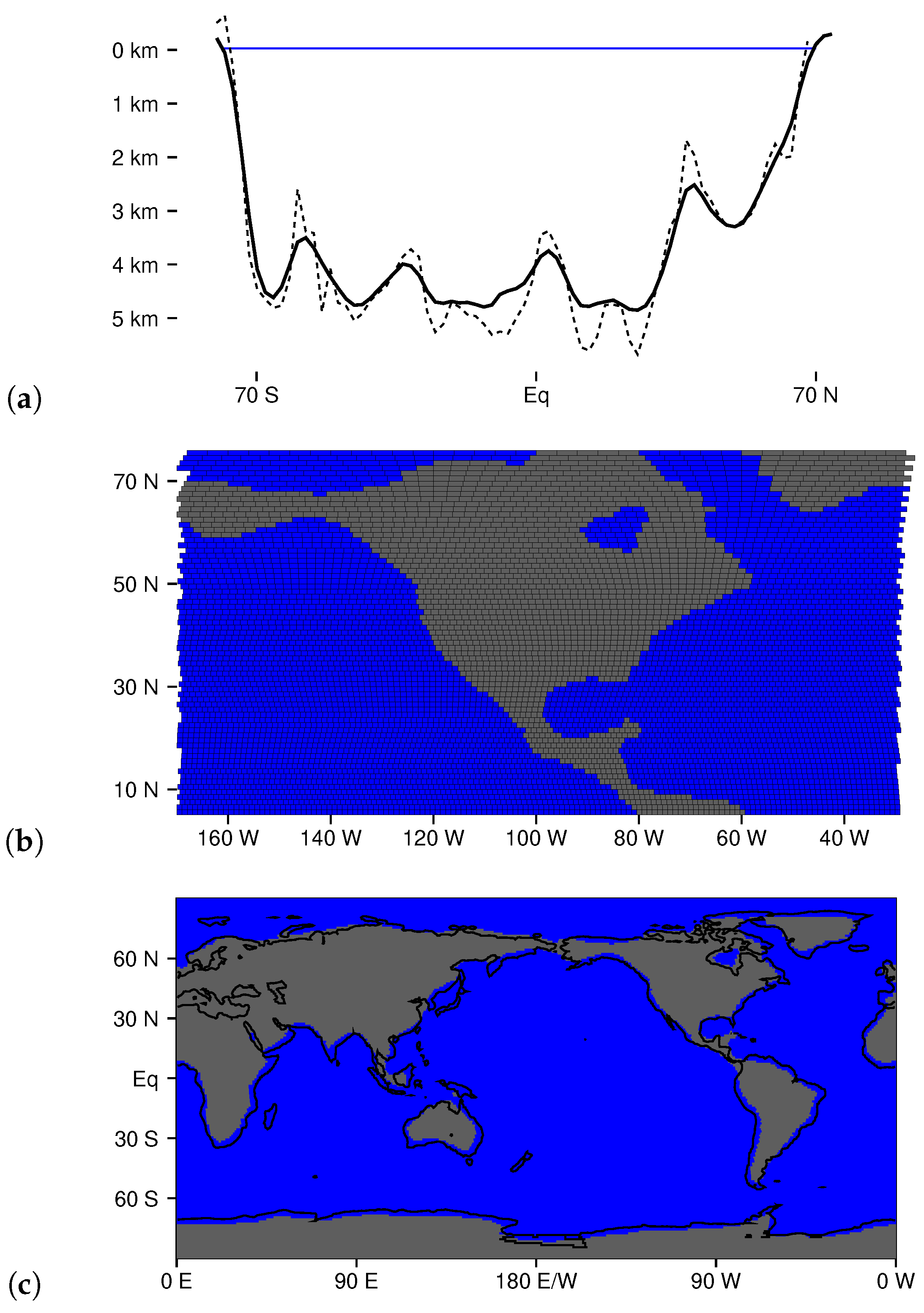
The Lagrangian method requires a specification of the bottom surface elevation over a horizontal grid of points on which Riemann sums are evaluated to calculate the pressure force [24]. For the simulations presented in this paper, the surface elevation field is constructed in the following way. First, actual mean surface height of the earth’s land surface and ocean bottom is averaged into 1-degree bins. Then, ocean depths are truncated at 4900 m, positive land surface values are set to 300 m, and the land mass of Central America is widened slightly. The resulting data are smoothed repeatedly using a 1-2-1 filter. Finally, the smoothed 1-degree data are averaged over the spherical grid of the ocean model. A comparison of the unsmoothed one-degree bathymetry (dashed) and the GLOM bottom topography (solid) is shown in Figure 3a for 30 W. Sharp topographic features are smoothed to be consistent with the large parcels used in this study, and the slope at the land ocean interface is reduced, which helps to improve numerical accuracy in low resolution simulations [25]. The land surface elevation is set to 300 m to prevent the smoothing of the bottom surface as well as the enhanced free surface height perturbations resulting from the use of gravity wave retardation [29] from overly distorting the locations of continental boundaries (e.g., from opening a water pathway through Central America).
The GLOM uses a spherical geometry in which grid boxes have a constant meridional width (in both degrees and meters), and a zonal width that is roughly the same in meters but increases in degrees longitude with distance from the equator. This geometry was first developed for a global Lagrangian atmospheric model by [4]. A mercator projection of the grid boxes is shown in Figure 3b for North America.
Here, grid boxes are shaded gray for z > 0 m, and blue for z < 0 m. A similar shading of model bathymetry is shown for the entire world in Figure 3c, with the z = 0 contour for actual bathymetry delineated with a black line. Notice that small peninsulas and islands are largely smoothed out in the GLOM’s bottom topography, but that the gross structure of continents and ocean basins is retained.
For the simulations discussed in this paper, grid boxes are 1 by 1 degrees wide at the equator, but have a larger width in degrees longitude at higher latitudes. Note that this grid is used to evaluate the pressure force and to create plots of layer thickness. In contrast, parcels span multiple grid boxes and move freely throughout the model domain. While it is difficult to precisely characterize the equivalent Eulerian resolution of a Lagrangian model, the author estimates it to be roughly 2 or 3 degrees at low latitudes, and somewhat coarser at high latitudes for the simulations presented in this paper.
2.6. Merging and Dividing Parcels
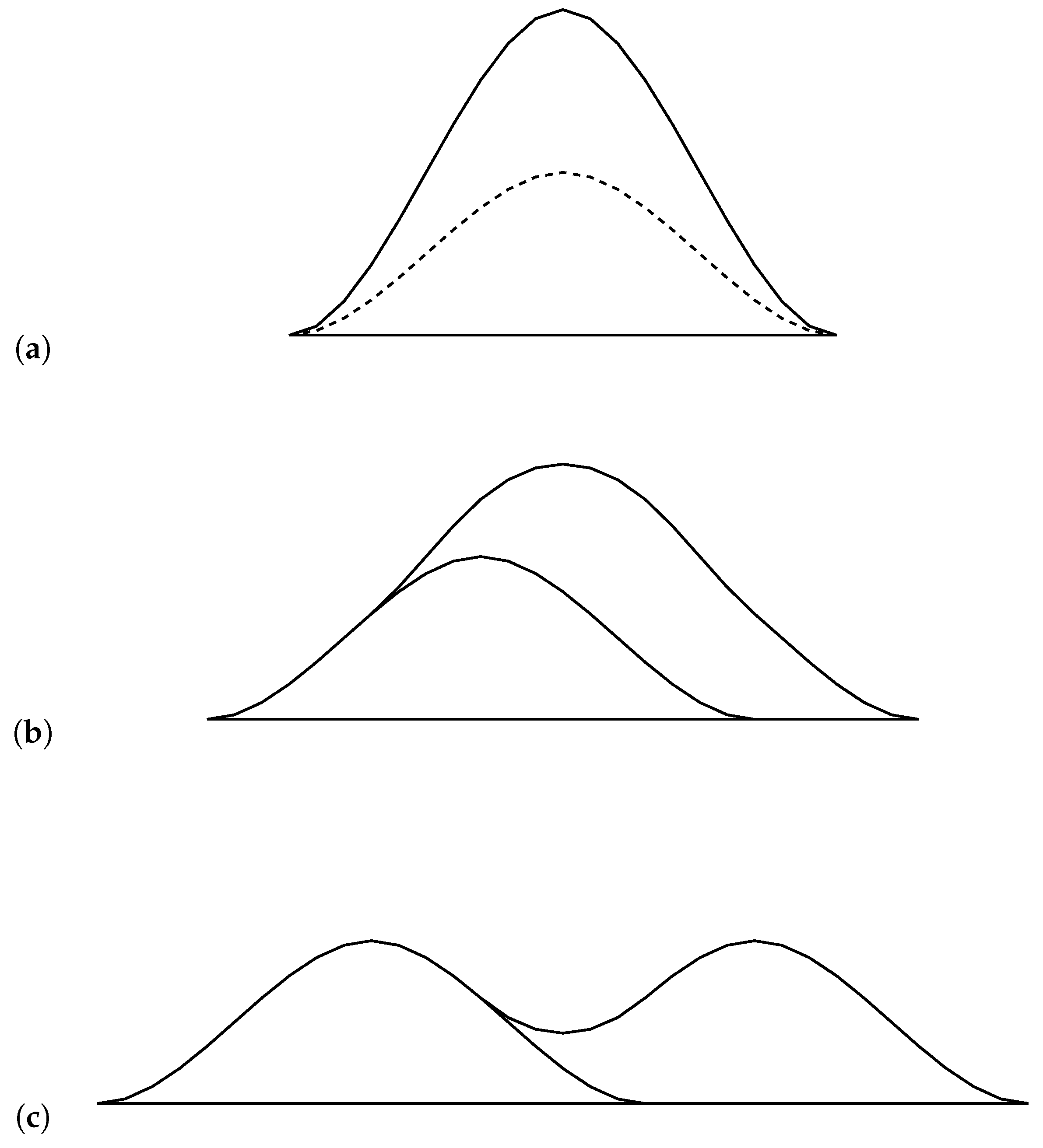
Following [25], the water in the oceans is divided into a collection of equally sized water mass elements (WMEs), which may be considered to be the building blocks of water parcels. The target size for parcels is one WME in the upper layer (0–700 m), two WMEs in the middle layer (700–2100 m), and four WMEs in the lower layer (depths greater than 2100 m). When a vertically thick parcel rises to a higher layer, and it is larger than the target size, it is sliced in half and the resulting two parcels begin moving independently (Figure 4).
When a vertically thin parcel sinks to a lower layer, it maintains its size until it overlaps and is sufficiently close to another vertically thin parcel, at which time the two parcels are combined (Figure 4, view panels from the bottom up). Notice that each individual WME has its own identification number, and it can be tracked through the dividing and merging process. While merging generates a small amount of numerical mixing, Haertel and Fedorov [15] found little difference between simulations with dividing and merging when compared to simulations with vertically thin parcels everywhere. Presumably, this is because merging only occurs when parcels go through substantial vertical displacements (i.e., it is a rare event). While dividing and merging can be turned off to completely remove numerical mixing of tracers, the author selected to use it here because it dramatically speeds up the model (by a factor of 2 or more for the simulations presented in this paper). Owing to the dividing and merging process, the vast majority of parcels in the upper layer comprise a single water mass element and have a vertical thickness of approximately 78 m, with a factor of 2 (4) increase in vertical thickness in the middle (lower) layer. All parcels have a radius of 333 km in each horizontal dimension (i.e., 3 degrees latitude and 3 degrees longitude near the equator). There are approximately 154,000 water mass elements in each simulation, which allows the model to be run for millennial time scales on a single processor (the GLOM has not yet been coded to run in parallel).
2.7. Experimental Design
In designing the simulations presented in this paper, the author had several goals: (1) to test the GLOM’s ability to reproduce the gross circulation and stratification structure of the world ocean; (2) to illustrate several unique capabilities of the GLOM that stem from its Lagrangian nature; and (3) to make a contribution to the field of physical oceanography. After reflecting on these goals, he chose to use the GLOM to extend the results of Haertel and Fedorov [15] (HF12) to include realistic topography and a global domain. Briefly, HF12 addressed the question of to what extent ocean circulation and stratification depend on interior mixing. They used a predecessor to the GLOM to simulate circulations in an idealized ocean with the scale of the Atlantic, and which included a circumpolar channel. They compared a simulation with a moderate amount of tracer mixing to one in which the tracer diffusivity was set to zero. They found that the leading order solution for ocean circulation, stratification, and heat transport could be reproduced with zero tracer diffusivity, and that interior mixing essentially contributed first-order perturbations to this solution. Accordingly, in this paper, we apply a surface forcing much like that used by HF12, but instead of using an idealized ocean basin, we use a global ocean with a smoothed version of actual bathymetry.
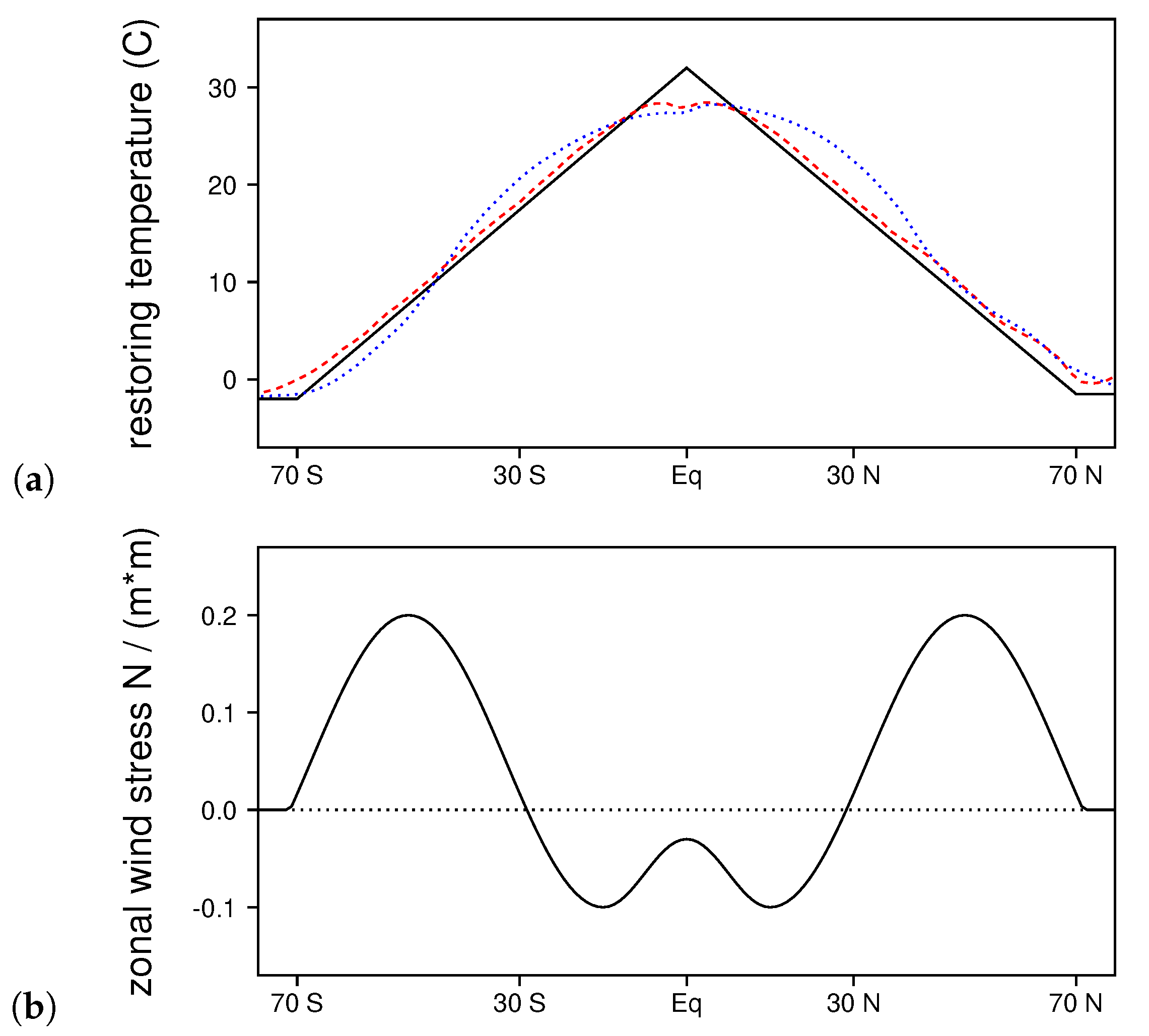
The temperature restoring function (Figure 5a, solid black line) is a piecewise linear function with a range set so that zonal average model SST (Figure 5a, red dashed line) has similar minima and maxima to that of zonal average SST in nature (Figure 5a, blue dotted line). Note that the restoring temperature is slightly lower in the Antarctic than in the Artic, which leads to Antarctic Bottom Water being more dense than North Atlantic Deep Water. The idealized zonal wind stress forcing (Figure 5b) is the same as that used by HF12; it includes strong westerlies at midlatitudes and weaker easterlies in the tropics.
The forcing was applied to an initially isothermal ocean (T = 0 °C) for a period of 1400 years. In one case, there was a moderately high vertical tracer diffusivity (1 cm2 s−1), and in the other case the diffusivity was zero. One minor adjustment was made after 500 years of model integration–the temperature difference between the restoring temperature in the Artic and Antartic was reduced from 1 °C to 0.5 °C to deepen the Atlantic Meridional Overturning Circulation (AMOC). By the year 1400, the simulation with interior mixing was in an approximately steady state in the upper ocean, with very weak cooling in the abyss. In the simulation without interior mixing, weak cooling continued in the deep ocean and abyss. However, the temperature here had reached within a few tenths of a degree of the minimum restoring temperature, limiting the amplitude of possible future temperature changes.
3. Results
When the GLOM is forced with the temperature restoring and wind stress functions described in the previous section (Figure 5), it generates large-scale circulation patterns and stratification that are similar to those in the world ocean in nature. In this section, we examine these structures, and compare results for the simulation with interior mixing to the one without, as well as both simulations to observations. The results generally support the main conclusion of HF12—that a model with zero tracer diffusivity can produce most of the large-scale circulation and stratification structure seen in nature (i.e., the zero-order solution), with interior mixing contributing first-order perturbations.
3.1. Horizontal Stream Function
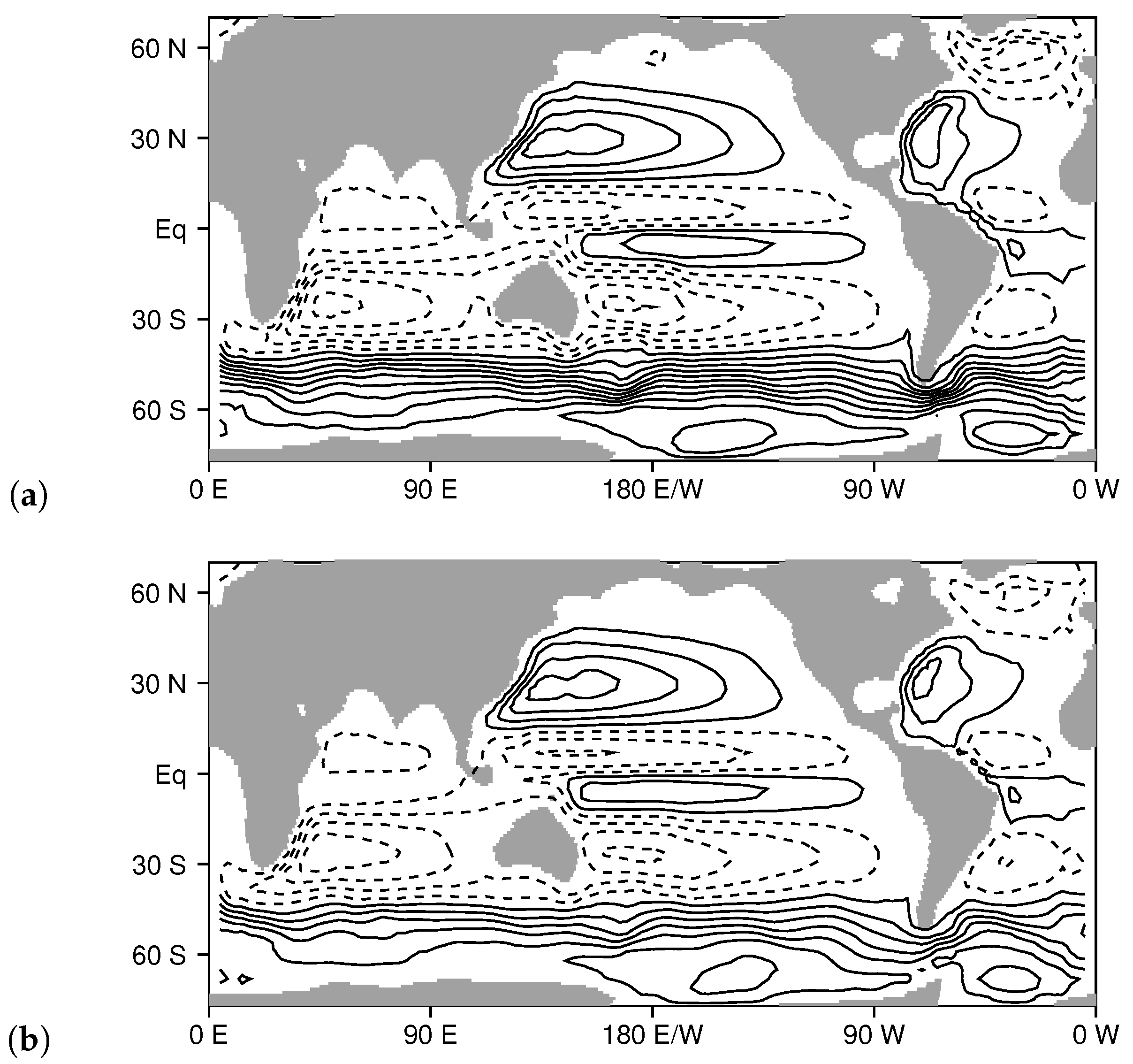
The horizontal circulation in the simulation with interior mixing (Figure 6a) is qualitatively consistent with that predicted by theory [30] for a forcing like that shown in Figure 5. Anticyclonic (cyclonic) gyres are present where the curl in the wind stress is negative (positive) with Sverdrup flow in the eastern portion of ocean basins, and more intense return flow in the form of western boundary currents to the east of continents. The model also produces an Antarctic Circumpolar Current (ACC), with gyres in the Ross and Weddell Seas. While the ACC is somewhat weaker than in nature [31], this is probably attributable to the low resolution of the model. In the simulation without mixing (Figure 6b), the overall flow structure is similar, but the amplitude of most gyres is slightly weaker, and the ACC is also weaker.
3.2. Surface Temperature Field
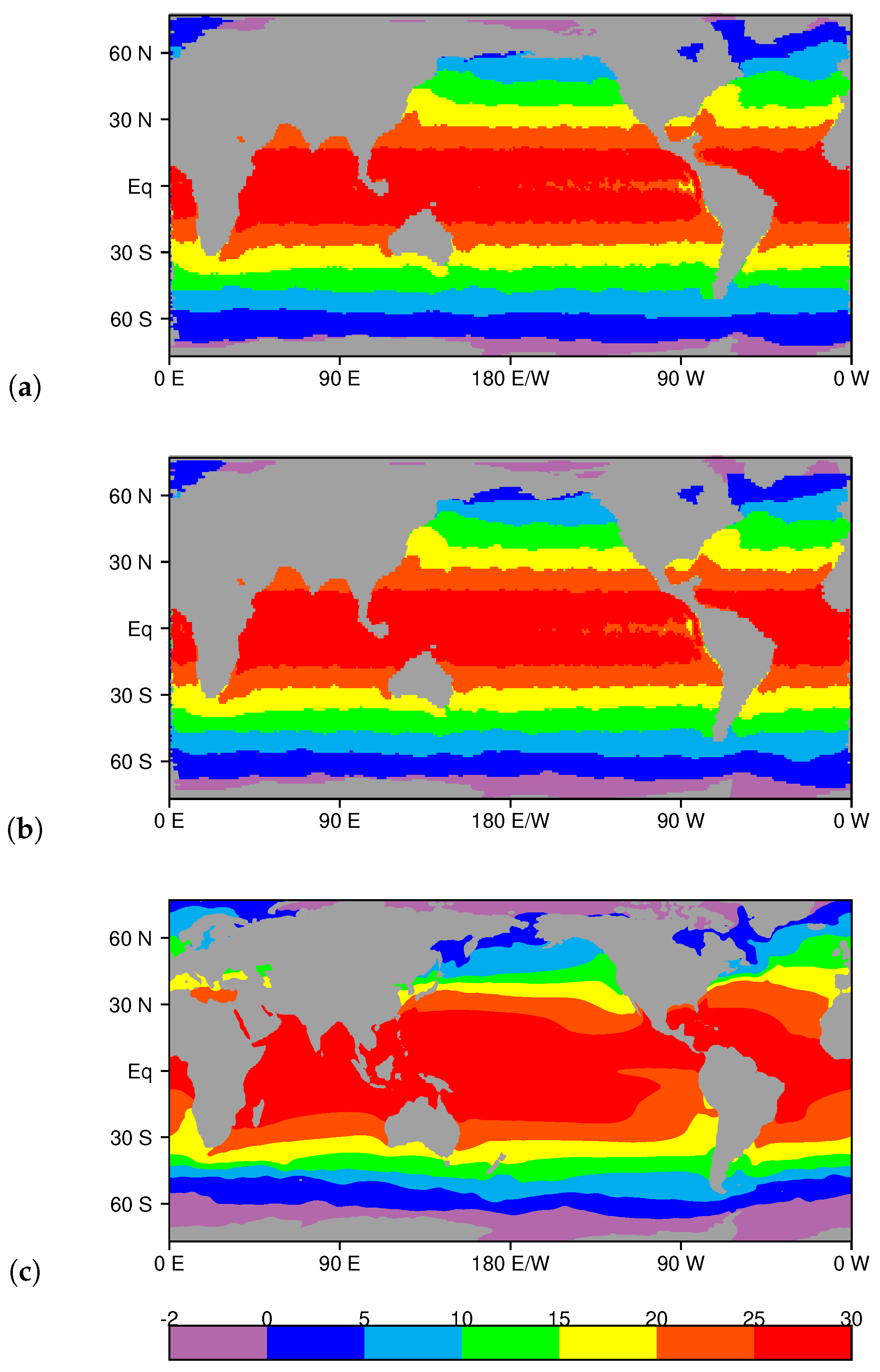
Despite the idealized nature of the GLOM and the forcing, it qualitatively captures many of the departures from zonal symmetry seen in the observed sea surface temperature (SST) field, including warm tongues protruding poleward at mid-latitudes along the eastern boundaries of North America, Asia, Africa, and South America, an equatorial cold tongue in the eastern Pacific, and isotherms that slope northward from west to east across the North Atlantic (Figure 7).
Of course, the low model resolution leads to western boundary currents that are broader and weaker than those observed in nature. Moreover, other features whose forcing is not included in the model are not well represented. For example, in nature, marine stratocumulus clouds are prevalent to the west of South America. They reflect a significant portion of the solar heating, reducing the SST there [32]. This forcing is not included in the GLOM simulations, and consequently SSTs are higher to the west of South America in the model (Figure 7a,b) than they are in nature (Figure 7c).
3.3. Stratification
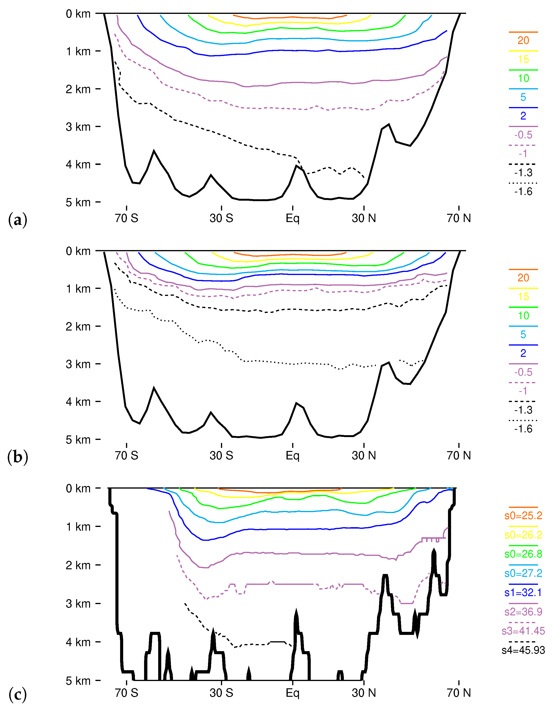
In the simulation with interior mixing, the GLOM generates a region of water that is substantially warmer than that in the rest of the ocean, which is largely contained in the upper 1 km between 50° S and 50° N (Figure 8a).
The vertical temperature gradient in the tropics within a few hundred meters of the surface is especially high. These aspects of the simulated thermocline structure are like those in the pycnocline in nature (Figure 8c). In both the model and in nature, the densest water forms in the Antarctic, and it undercuts the deep water formed in the north (Figure 8a,c). When interior tracer mixing is removed, the upper thermocline structure is very similar to that in the simulation with mixing (Figure 8b). However, at greater depths, the ocean warms substantially, with many isotherms rising around 1 km or more. The two simulations (with and without the mixing of tracers), have a similar slope in most of the Atlantic (Figure 8a,b), which is also similar to that of isopycnals in nature (Figure 8c).
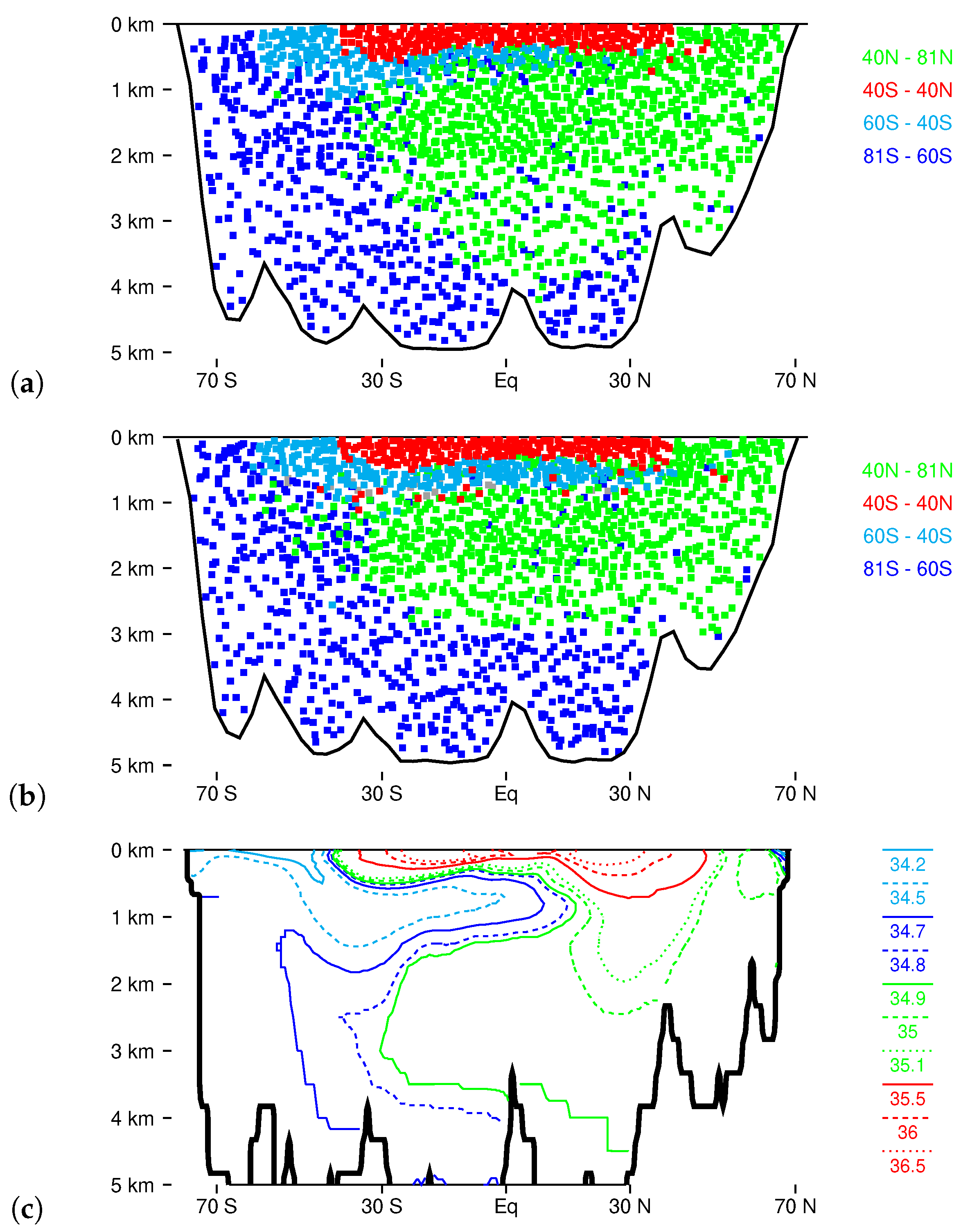
3.4. Water Mass Distributions
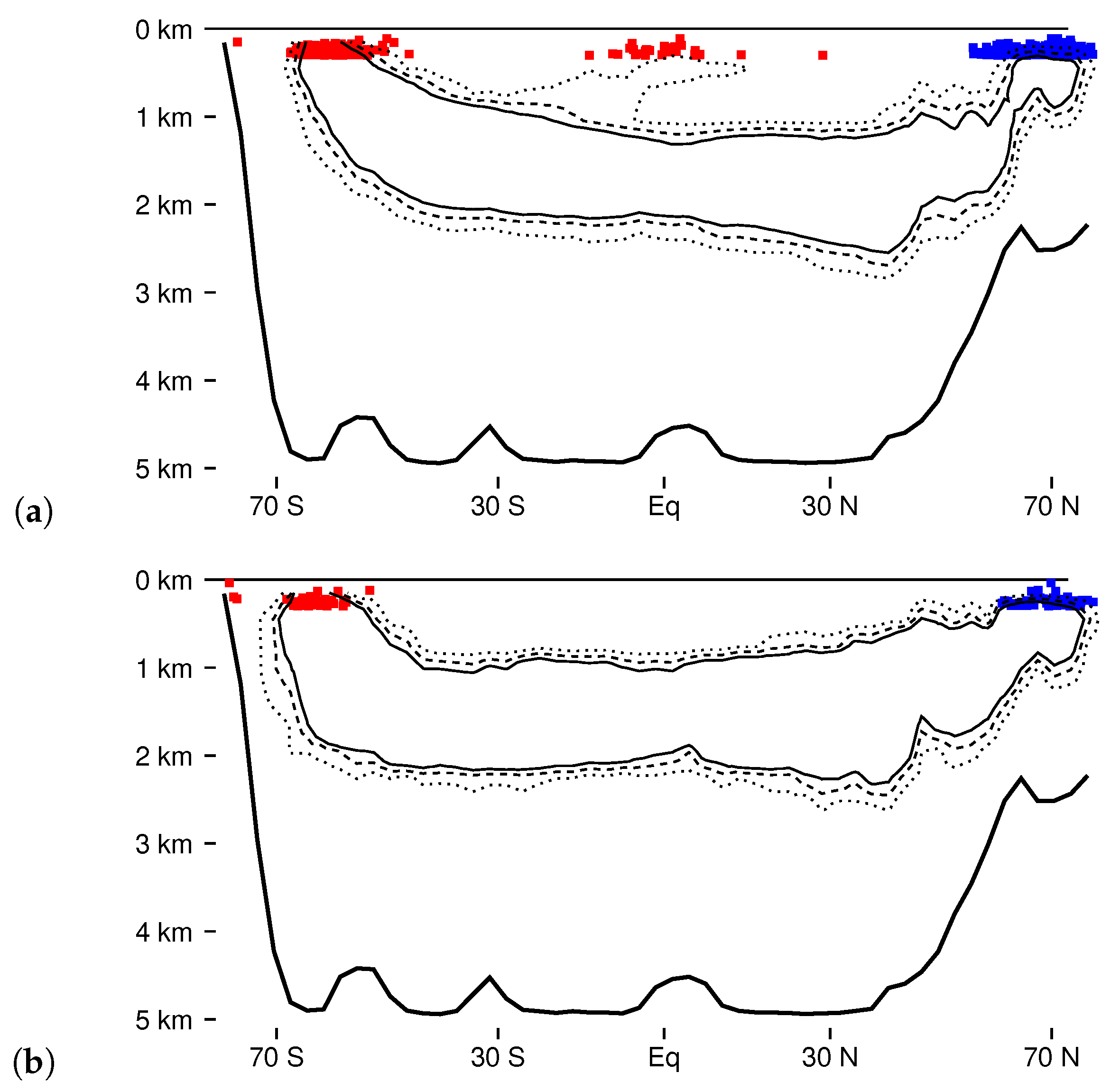
One advantage of the GLOM is that it is easy to identify locations where water masses form. In Figure 9, we color code parcels along 30° W by the latitude at which they were last modified by the surface forcing (the model saves this information as a parcel variable and updates it it every time surface fluxes alter the parcel temperature). We compare the water masses in the GLOM (Figure 9a,b) to those in nature, as revealed by the salinity field (Figure 9c). In the simulation with mixing, each of the main water masses in the Atlantic is represented (Figure 9a): warm tropical and sub-tropical water near the surface that forms between 40° S and 40° N (red dots); Antarctic Intermediate Water (AIW) that forms between 40° and 60° S and moves northward along the main thermocline (cyan dots); North Atlantic Deep Water (NADW) that forms north of 40° N and reaches depths of about 4 km (green dots), and Antarctic Bottom Water (ABW) that forms south of 60° S, and spreads to cover most of the ocean bottom. Each of these water masses has a similar positioning to its counterpart in nature (Figure 9c), as inferred from the salinity field. In the simulation without tracer diffusion (Figure 9b), the general distribution of water masses is similar, except that the AIW penetrates farther north, the NADW is shallower, and the ABW is deeper.
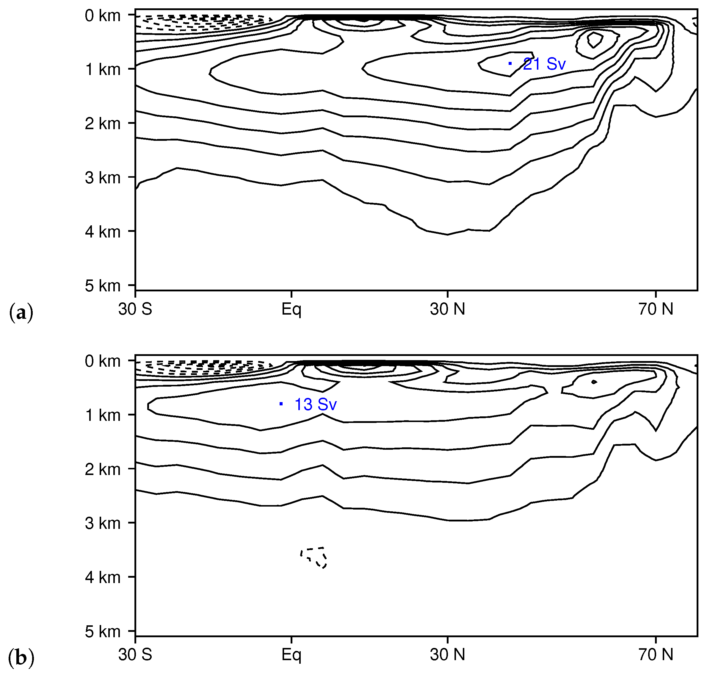
3.5. Atlantic Meridional Overturning Circulation
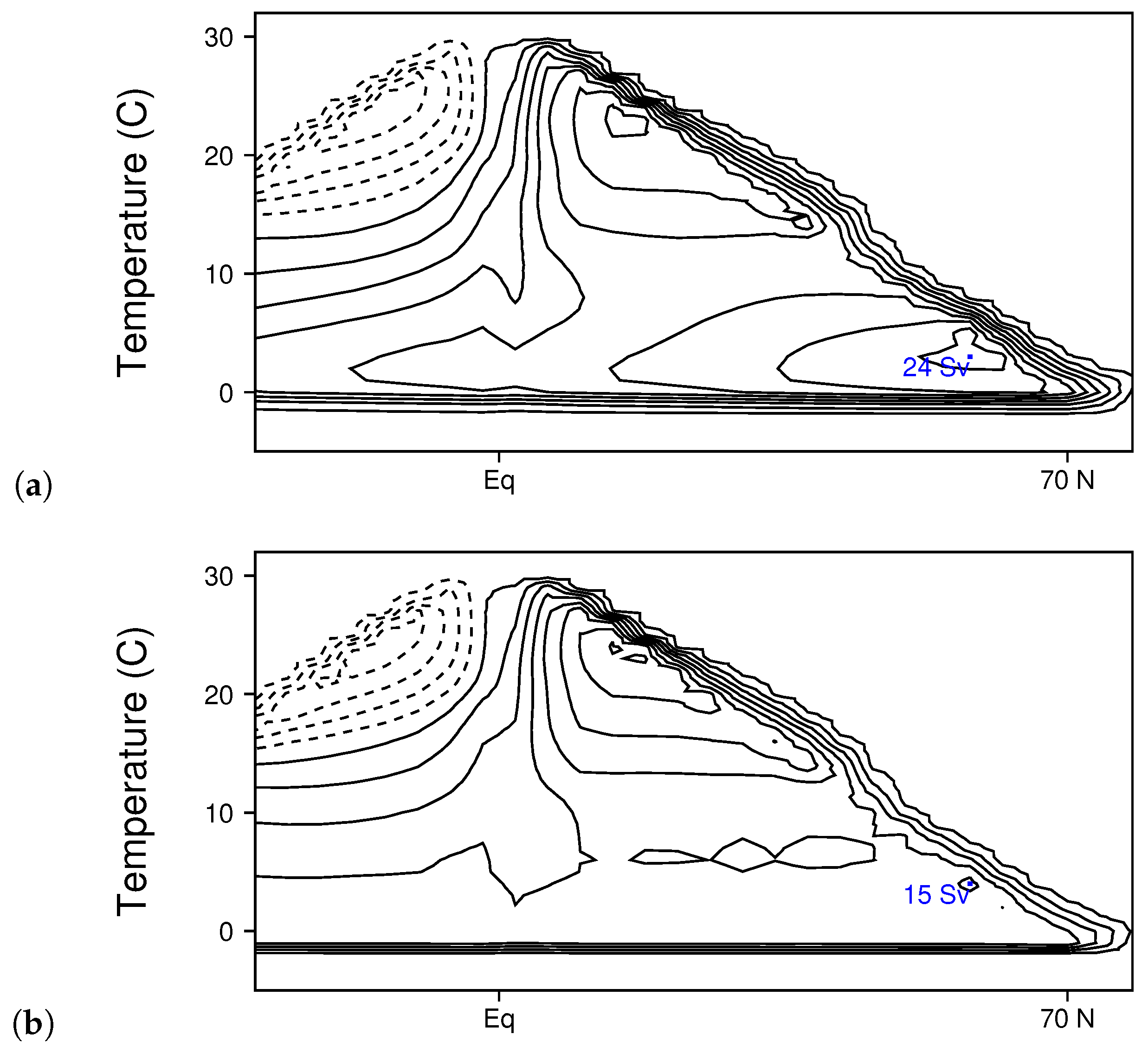
Most of the deep overturning the model generates is in the Atlantic Ocean, and we now examine this circulation in detail, both because of its importance to ocean heat transport and to follow up on the previous Lagrangian modeling results of HF12. When interior mixing is included in the model, the AMOC has a mid-latitude amplitude of about 21 Sv (Figure 10a), of which about 11 Sv upwells in the Southern Ocean. When interior tracer mixing is removed, the peak amplitude of the overturning is reduced to 13 Sv, but almost as much water (10 Sv) upwells in the Southern Ocean (Figure 10b). The overturning also becomes more shallow, with the deepest streamlines reaching around 3 km. The other difference is that there is a lack of streamlines crossing the thermocline between 27° S and 40° N. We also examine the AMOC using temperature as a vertical coordinate in Figure 11—both because this more directly illustrates heat transport by removing adiabatic overturning cells [15,33], and because it also more clearly illustrates shallow wind-driven cells. When interior mixing is included, the GLOM generates 24 Sv of deep overturning in the North Atlantic (Figure 11a), with roughly 12 Sv of water upwelling in the Southern Ocean. There is little temperature change following four streamlines (each representing 3 Sv of transport) from 70° N to 30° S. However, multiple streamlines indicate warming of water in the interior of the deep cell with roughly 6 Sv of upwelling near the equator (Figure 11a). When interior mixing is removed (Figure 11b), the amplitude of the deep cell is reduced to 15 Sv, but once again roughly 12 Sv of water sinks in the North Atlantic and makes a long journey to the Southern Ocean with very little temperature change. Also note that removing interior mixing has little impact on the shallow wind-driven cells for T > 10 °C. These results suggest that the basic character of the AMOC is maintained without interior mixing, but that mixing deepens the circulation, and generates transport across the equatorial thermocline.
3.6. Sample Trajectory Analysis
One advantage of the GLOM is that it provides trajectory information for every wass mass element (WME) in the ocean. Each WME has a unique identification number (ID) that does not change during the course of a simulation. To compute a trajectory for a given WME, the modeler simply uses the ID to look up parcel positions for that WME for the times that data is saved. Moreover, for low-resolution runs, it is easy to construct trajectories for every WMI in the ocean. These can then be objectively partitioned to illustrate particular water pathways. We now perform such an analysis for the subsurface pathway of the AMOC.
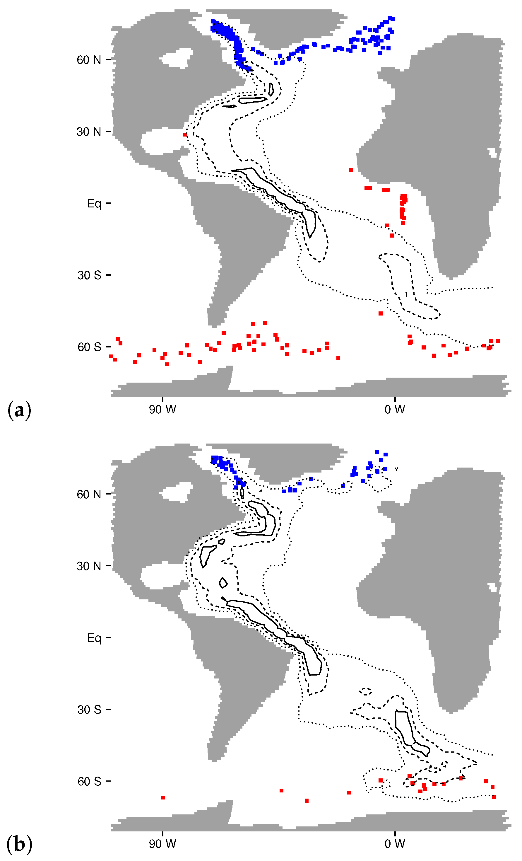
Figure 12a shows downwelling (blue) and upwelling (red) locations of all WMEs that sink in the North Atlantic and upwell south of 30 N during the last 300 years of simulation with interior mixing. Water generally sinks (i.e., loses contact with the surface) in the Labrador or Norwegian Seas and upwells (i.e., regains contact with the surface) near the Gulf of Guinea or in the Southern Ocean. Regions most frequented by WMEs are contoured, revealing that the preferred pathway to upwelling is through a deep western boundary current just to the east of the Americas, which takes an eastward turn south of 20° S (see dashed and solid black contours in Figure 12a). When interior tracer mixing is removed, the downwelling locations are similar, as is the preferred pathway to the Southern Ocean, but water no longer upwells near the Equator (Figure 12b). Presumably, this is because without interior mixing, there is no longer any mechanism to warm the water once it loses contact with the surface, which would be necessary for equatorial upwelling.
A y–z cross-section of the water pathways in shown in Figure 13.
In both simulations, water typically downwells just south of 70° N, and upwells near 60° S. In the simulation with interior tracer mixing, the pathway to upwelling is slightly deeper (Figure 13a), and includes a branch to equatorial upwelling that is not present in the simulation without interior mixing (Figure 13b). The pathways shown in Figure 12 and Figure 13 are generally consistent with the streamfunctions shown in Figure 10; although the preferred pathway to upwelling is slightly shallower than the streamlines indicate, which may indicate a bias towards shallower paths because of the relatively short sampling time (300 years).
3.7. Pacific Water Masses
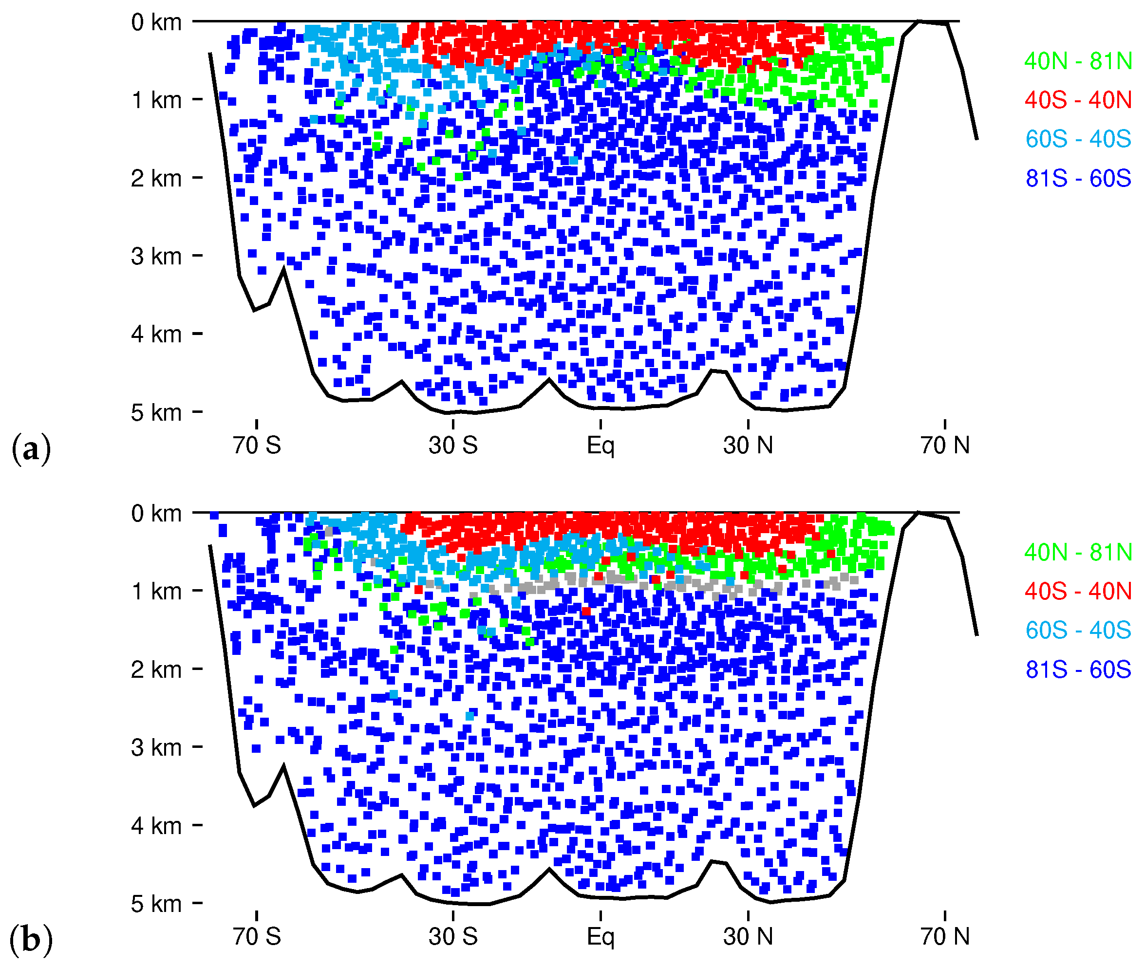
As in nature, the deep circulation in the GLOM in the Pacific Ocean differs greatly to how it is in the Atlantic Ocean. In particular, for both the simulations, with and without interior mixing, Antarctic Bottom Water fills almost all of the ocean at depths greater than 1 km (Figure 14). In the southern hemisphere, there are a few scattered parcels of North Atlantic Deep Water (green dots) at depths between 1 and 2 km that apparently come around the southern tip of Africa and through the Indian Ocean to reach the central Pacific. We conclude that there is essentially no deep water formation in the Pacific in the GLOM, which is not surprising considering the ocean geometry (Figure 3b) and the zonally symmetric temperature restoring (Figure 5b).
4. Discussion
In this paper, the author combines components of a Lagrangian basin-scale ocean model with the dynamical core of a global Lagrangian atmospheric model to create a new global Lagrangian ocean model (GLOM). Rather than numerically solving partial differential equations that describe fluid flow, this model predicts the motions of individual fluid parcels using ordinary differential equations and classical physics. The GLOM has variable bottom topography and spherical geometry, so it can be used to simulate general circulations of the global ocean. It also has a unique convective parameterization, in which the vertical positions of parcels are sorted by density to remove convective instability.
When forced with idealized surface temperature restoring and wind stress, the GLOM generates much of the circulation structure seen in nature in the global oceans, including mid-latitude gyres with western boundary currents, shallow wind-driven cells at low latitudes, a deep overturning in the Atlantic Ocean, and an Antarctic Circumpolar Current. The GLOM also produces thermocline structure and water mass distributions that are similar to those seen in nature. When interior mixing is removed, the large-scale ocean circulation, stratification, and water mass distributions are similar, with the main difference being that circulations, thermocline structure and upper-level water masses are slightly shallower. These results support the primary conclusion of [15] (and earlier papers such as [34,35]) that the leading-order solution for ocean stratification and circulation can be reproduced without interior tracer mixing, and that including tracer diffusivity creates first-order perturbations.
The work presented here and in previous Lagrangian modeling studies supports the idea that the Lagrangian approach would complement existing numerical methods used to study climate dynamics and climate change. This paper highlights several unique features of the GLOM: (1) the ability to conduct simulations with zero tracer diffusivity; (2) the unique convective parameterization which restacks parcels in convectively unstable regions, and (3) ease in tracking every mass element in the ocean and determining locations where water masses form. For these reasons, the author is continuing to refine and improve the GLOM, and he will soon be coupling it to a Lagrangian atmospheric model for coupled ocean–atmosphere climate dynamics experiments.
Of course, the GLOM has a number of disadvantages as well, so it would not be well suited for every climate application. For example, the model, as it is currently configured, uses a high degree of gravity wave retardartion (GWR) [29] which amounts to assuming that there is a layer of fluid above the ocean with a density slightly lower than that of salt water, and which slows externing gravity waves, allowing the model to have a large time step. The main side effect of GWR is that it greatly enhances the amplitude of free surface perturbations, which would be a problem for modeling circulations in shallow estuaries, for example. A second drawback to the Lagrangian approach used here is that there is a potential energy barrier to starting circulations in a pile of parcels [25], so it could have problems simulating weakly forced circulations.
The simulations presented in this paper are also limited in the sense that they use very large water parcels, with horizontal scales of a few degrees, and vertical scales on the order of 100 m. Owing to the lack of numerical tracer diffusion in the model, the equivalent resolution in an Eulerian ocean model is probably somewhat finer. For example, Haertel et al. [25] found that circulations and stratification in a 3-degree basin-scale Lagrangian ocean model compared favorably to those in a 1-degree z-coordinate model that was exposed to the same surface forcing. However, this resolution is still very coarse, and it represents the low end of expected climate applications (i.e., for millennial time-scale, single-processor, global simulations). Fortunately, there is reason to believe that the GLOM will have the capacity to be run at much finer resolution once it is coded in parallel. For example, Haertel et al. [24] found nearly linear scaling in a predecessor to the GLOM, which had similar computational costs to a sigma-coordinate ocean model for simulating circulations in a large lake. Moreover, it is encouraging that even at the very coarse resolution used in this paper, the GLOM was able to reproduce the gross circulation patterns and stratification seen in the world ocean, with the Lagrangian convective parameterization and random parcel motions apparently adequately representing buoyancy driven convective circulations and mesoscale eddy transports that occur at much smaller scales in nature.
Considering that the GLOM is in a relatively early stage of development when compared with other climate modeling tools, it is too early to fully understand its advantages and disadvantages at this time. Moreover, there are probably many other potential applications for the GLOM and its fully Lagrangian atmospheric counterpart that will take years to explore. For example, the recent study of Paparella and Popolizio [36] suggests that Lagrangian models will have advantages for simulating the mixing of biogeochemical tracers. However, one thing is clear already—Lagrangian models, as well as the physical parameterizations that go along with them, are fundamentally different from Eulerian models and methods, and they make a significant contribution to the diversity of climate modeling tools.
Funding
This research was supported by NSF grant AGS-1561066.
Conflicts of Interest
The author declares no conflict of interest.
References
- Lin, J.; Brunner, D.; Gerbig, C.; Stohl, A.; Luhar, A.; Webley, P. Lagrangian Modeling of the Atmosphere; John Wiley & Sons: Hoboken, NJ, USA, 2013; Volume 200. [Google Scholar]
- Bates, M.L.; Griffies, S.M.; England, M.H. A dynamic, embedded Lagrangian model for ocean climate models. Part I: Theory and implementation. Ocean Model. 2012, 59, 41–59. [Google Scholar] [CrossRef]
- Van Sebille, E.; Griffies, S.M.; Albernathey, R.; Adams, T.P.; Befloff, P.; Biastoch, A.; Blanke, B.; Chassignet, E.P.; Cheng, Y.; Cotter, C.J.; et al. Lagrangian ocean analysis: Fundamentals and practices. Ocean Model. 2018, 121, 49–75. [Google Scholar] [CrossRef]
- Haertel, P.; Boos, W.R.; Straub, K. Origins of Moist Air in Global Lagrangian Simulations of the Madden—Julian Oscillation. Atmosphere 2017, 8, 158. [Google Scholar] [CrossRef]
- Haertel, P.; Straub, K.; Fedorov, A. Lagrangian overturning and the Madden–Julian Oscillation. Q. J. R. Meteorol. Soc. 2014, 140, 1344–1361. [Google Scholar] [CrossRef]
- Haertel, P.; Straub, K.; Budsock, A. Transforming circumnavigating Kelvin waves that initiate and dissipate the Madden–Julian Oscillation. Q. J. R. Meteorol. Soc. 2015, 141, 1586–1602. [Google Scholar] [CrossRef]
- Zhang, C. Madden-julian oscillation. Rev. Geophys. 2005, 43. [Google Scholar] [CrossRef]
- Slingo, J.; Rowell, D.; Sperber, K.; Nortley, F. On the predictability of the interannual behaviour of the Madden-Julian Oscillation and its relationship with El Niño. Q. J. R. Meteorol. Soc. 1999, 125, 583–609. [Google Scholar] [CrossRef]
- Lin, J.L.; Kiladis, G.N.; Mapes, B.E.; Weickmann, K.M.; Sperber, K.R.; Lin, W.; Wheeler, M.C.; Schubert, S.D.; Del Genio, A.; Donner, L.J.; et al. Tropical intraseasonal variability in 14 IPCC AR4 climate models. Part I: Convective signals. J. Clim. 2006, 19, 2665–2690. [Google Scholar] [CrossRef]
- Hung, M.P.; Lin, J.L.; Wang, W.; Kim, D.; Shinoda, T.; Weaver, S.J. MJO and convectively coupled equatorial waves simulated by CMIP5 climate models. J. Clim. 2013, 26, 6185–6214. [Google Scholar] [CrossRef]
- Maloney, E.D.; Hartmann, D.L. Modulation of eastern North Pacific hurricanes by the Madden–Julian oscillation. J. Clim. 2000, 13, 1451–1460. [Google Scholar] [CrossRef]
- Fedorov, A.V.; Hu, S.; Lengaigne, M.; Guilyardi, E. The impact of westerly wind bursts and ocean initial state on the development, and diversity of El Niño events. Clim. Dyn. 2015, 44, 1381–1401. [Google Scholar] [CrossRef]
- Wu, M.L.C.; Schubert, S.; Huang, N.E. The development of the South Asian summer monsoon and the intraseasonal oscillation. J. Clim. 1999, 12, 2054–2075. [Google Scholar] [CrossRef]
- Neena, J.; Lee, J.Y.; Waliser, D.; Wang, B.; Jiang, X. Predictability of the Madden–Julian oscillation in the intraseasonal variability hindcast experiment (ISVHE). J. Clim. 2014, 27, 4531–4543. [Google Scholar] [CrossRef]
- Haertel, P.; Fedorov, A. The ventilated ocean. J. Phys. Oceanogr. 2012, 42, 141–164. [Google Scholar] [CrossRef]
- Griffies, S.M.; Pacanowski, R.C.; Hallberg, R.W. Spurious diapycnal mixing associated with advection in az-coordinate ocean model. Mon. Weather Rev. 2000, 128, 538–564. [Google Scholar] [CrossRef]
- Bleck, R. An oceanic general circulation model framed in hybrid isopycnic-Cartesian coordinates. Ocean Model. 2002, 4, 55–88. [Google Scholar] [CrossRef]
- Riehl, H. On the heat balance of the equatorial trough zone. Geophysica 1958, 6, 503–538. [Google Scholar]
- Zipser, E.J. The role of organized unsaturated convective downdrafts in the structure and rapid decay of an equatorial disturbance. J. Appl. Meteorol. 1969, 8, 799–814. [Google Scholar] [CrossRef]
- Haertel, P.T.; Randall, D.A. Could a pile of slippery sacks behave like an ocean? Mon. Weather Rev. 2002, 130, 2975–2988. [Google Scholar] [CrossRef]
- Daly, B.; Harlow, F.; Welch, J.; Wilson, E.; Sanmann, E. Numerical Fluid Dynamics Using the Particle-and-Force Method. Part I. the Method and Its Applications; Technical Report; Los Alamos Scientific Lag., Univ. California: Oakland, CA, USA, 1964. [Google Scholar]
- Monaghan, J.J. Smoothed particle hydrodynamics. Annu. Rev. Astron. Astrophys. 1992, 30, 543–574. [Google Scholar] [CrossRef]
- Pavia, E.G.; Cushman-Roisin, B. Modeling of oceanic fronts using a particle method. J. Geophys. Res. Oceans 1988, 93, 3554–3562. [Google Scholar] [CrossRef]
- Haertel, P.T.; Randall, D.A.; Jensen, T.G. Simulating upwelling in a large lake using slippery sacks. Mon. Weather Rev. 2004, 132, 66–77. [Google Scholar] [CrossRef]
- Haertel, P.T.; Van Roekel, L.; Jensen, T.G. Constructing an idealized model of the North Atlantic Ocean using slippery sacks. Ocean Model. 2009, 27, 143–159. [Google Scholar] [CrossRef]
- Van Roekel, L.P.; Ito, T.; Haertel, P.T.; Randall, D.A. Lagrangian analysis of the meridional overturning circulation in an idealized ocean basin. J. Phys. Oceanogr. 2009, 39, 2175–2193. [Google Scholar] [CrossRef]
- Haertel, P. A Lagrangian method for simulating geophysical fluids. Lagrangian Model. Atmos. 2012, 85–98. [Google Scholar] [CrossRef]
- Gent, P.R.; Mcwilliams, J.C. Isopycnal mixing in ocean circulation models. J. Phys. Oceanogr. 1990, 20, 150–155. [Google Scholar] [CrossRef]
- Jensen, T.G. Artificial retardation of barotropic waves in layered ocean models. Mon. Weather Rev. 1996, 124, 1272–1284. [Google Scholar] [CrossRef]
- Pedlosky, J. Ocean Circulation Theory; Springer Science & Business Media: Berlin, Germany, 2013. [Google Scholar]
- Cunningham, S.; Alderson, S.; King, B.; Brandon, M. Transport and variability of the Antarctic circumpolar current in drake passage. J. Geophys. Res. Oceans 2003, 108. [Google Scholar] [CrossRef]
- De Szoeke, S.P.; Yuter, S.; Mechem, D.; Fairall, C.W.; Burleyson, C.D.; Zuidema, P. Observations of stratocumulus clouds and their effect on the eastern Pacific surface heat budget along 20 S. J. Clim. 2012, 25, 8542–8567. [Google Scholar] [CrossRef]
- Döös, K.; Nycander, J.; Coward, A.C. Lagrangian decomposition of the Deacon Cell. J. Geophys. Res. Oceans 2008, 113. [Google Scholar] [CrossRef]
- Luyten, J.; Pedlosky, J.; Stommel, H. The ventilated thermocline. J. Phys. Oceanogr. 1983, 13, 292–309. [Google Scholar] [CrossRef]
- Welander, P. An advective model of the ocean thermocline. Tellus 1959, 11, 309–318. [Google Scholar] [CrossRef]
- Paparella, F.; Popolizio, M. Lagrangian numerical methods for ocean biogeochemical simulations. J. Comput. Phys. 2018, 360, 229–246. [Google Scholar] [CrossRef]
Figure 1.
Parcel vertical thickness function (i.e., the outline of a parcel on a level surface).

Figure 2.
A schematic illustration of the Lagrangian convective parameterization. (a) A collection of water parcels, each having the same vertical thickness function, with darker shading denoting denser parcels. (b) The density of the top middle parcel (P) increases (e.g., from a temperature decrease or a salinity increase) yielding an unstable stratification. (c) The convective parameterization changes the stacking order of the parcels, so parcel P sinks to the level at which its density is the same as neighboring parcels. The long dashed line shows the path of the parcel center. Surrounding parcels rise slightly with short dashed lines illustrating the paths of parcel centers.

Figure 3.
Bottom topography and spherical geometry. (a) Model bottom surface along 30 W (solid black line), the observed bathymetry (dashed line), and the undisturbed free surface height (blue). (b) Spherical geometry for North America. Each grid box used for calculating the pressure force is outlined in black. (c) Regions of land (gray) and ocean (blue) as determined by the zero height contour. The solid black line denotes the actual position of the land–sea interface.

Figure 4.
Dividing and merging parcels. (a) A single parcel comprising two water mass elements. (b,c) The parcel divides into two smaller parcels each comprising one water mass element, which then move independently. Viewing the panels in reverse order illustrates the merging process.
Figure 4.
Dividing and merging parcels. (a) A single parcel comprising two water mass elements. (b,c) The parcel divides into two smaller parcels each comprising one water mass element, which then move independently. Viewing the panels in reverse order illustrates the merging process.

Figure 5.
Surface forcing. (a) restoring temperature (solid black line), average SST in the simulation with mixing (red dotted line), and observed average SST (blue dotted line), which is from the NCEP Optimally Interpolated weekly SST and Sea Ice datasets for the years 1998–2009. (b) zonal wind stress.

Figure 6.
Horizontal streamfunction (10 Sv contour interval). (a) Simulation with interior mixing. (b) Simulation without interior mixing. Positive (negative) contours are drawn with solid (dashed) lines, with contour values ranging from −45 to 105 Sv.
Figure 6.
Horizontal streamfunction (10 Sv contour interval). (a) Simulation with interior mixing. (b) Simulation without interior mixing. Positive (negative) contours are drawn with solid (dashed) lines, with contour values ranging from −45 to 105 Sv.

Figure 7.
Sea surface temperature (°C). (a) Simulation with mixing. (b) Simulation without mixing. (c) Observed.
Figure 7.
Sea surface temperature (°C). (a) Simulation with mixing. (b) Simulation without mixing. (c) Observed.

Figure 8.
Stratification along 30° W. (a) Temperature (°C) in the simulation with mixing. (b) Temperature (°C) in the simulation without mixing. (c) Potential density in nature, with the upper four isopycals referenced to the surface, and the lower four isopycnals referenced to their approximate depths. The lower isopycnals are shown only in the vicinity of the depth to which they are referenced.

Figure 9.
Water masses along 30° W. Parcels are color coded by the latitude of last surface contact in (a) the simulation with mixing. and (b) the simulation without mixing. (c) Observed water masses are inferred from the salinity field.
Figure 9.
Water masses along 30° W. Parcels are color coded by the latitude of last surface contact in (a) the simulation with mixing. and (b) the simulation without mixing. (c) Observed water masses are inferred from the salinity field.

Figure 10.
Meridional overturning streamfunction (3 Sv contour interval). (a) Simulation with mixing. (b) Simulation without mixing. Positive (negative) contours are drawn with solid (dashed) lines, with contour values ranging from −10.5 to 22.5 Sv.
Figure 10.
Meridional overturning streamfunction (3 Sv contour interval). (a) Simulation with mixing. (b) Simulation without mixing. Positive (negative) contours are drawn with solid (dashed) lines, with contour values ranging from −10.5 to 22.5 Sv.

Figure 11.
Meridional overturning streamfunction with temperature as a vertical coordinate (3 Sv contour interval). (a) Simulation with mixing. (b) Simulation without mixing. Positive (negative) contours are drawn with solid (dashed) lines, with contour values ranging from −10.5 to 22.5 Sv.
Figure 11.
Meridional overturning streamfunction with temperature as a vertical coordinate (3 Sv contour interval). (a) Simulation with mixing. (b) Simulation without mixing. Positive (negative) contours are drawn with solid (dashed) lines, with contour values ranging from −10.5 to 22.5 Sv.

Figure 12.
Horizontal pathway to upwelling of North Atlantic Deep Water. (a) Simulation with mixing. (b) Simulation without mixing. Blue (Red) dots indicated downwelling (upwelling) locations. Contouring indicates the percent of WME pathways that pass through each 3 by 3 degree grid box (10, 30, and 50 percent).

Figure 13.
Vertical cross-section of pathway to upwelling of North Atlantic Deep Water. (a) Simulation with mixing. (b) Simulation without mixing. Blue (red) dots indicate downwelling (upwelling) locations. Contouring indicates the percent of WME pathways that pass through each 3 degree by 300 m grid box (10, 30, and 50 percent).

Figure 14.
Water masses along 170° W. Parcels are color coded by the latitude of last surface contact in (a) the simulation with mixing, and (b) the simulation without mixing.
Figure 14.
Water masses along 170° W. Parcels are color coded by the latitude of last surface contact in (a) the simulation with mixing, and (b) the simulation without mixing.

© 2019 by the author. Licensee MDPI, Basel, Switzerland. This article is an open access article distributed under the terms and conditions of the Creative Commons Attribution (CC BY) license (http://creativecommons.org/licenses/by/4.0/).
Share and Cite
MDPI and ACS Style
Haertel, P. A Lagrangian Ocean Model for Climate Studies. Climate 2019, 7, 41. https://doi.org/10.3390/cli7030041
AMA Style
Haertel P. A Lagrangian Ocean Model for Climate Studies. Climate. 2019; 7(3):41. https://doi.org/10.3390/cli7030041
Chicago/Turabian StyleHaertel, Patrick. 2019. "A Lagrangian Ocean Model for Climate Studies" Climate 7, no. 3: 41. https://doi.org/10.3390/cli7030041
APA StyleHaertel, P. (2019). A Lagrangian Ocean Model for Climate Studies. Climate, 7(3), 41. https://doi.org/10.3390/cli7030041
Note that from the first issue of 2016, this journal uses article numbers instead of page numbers. See further details here.