Article

Not so Normal Normals: Species Distribution Model Results are Sensitive to Choice of Climate Normals and Model Type

by
Catherine S. Jarnevich
1,* and
Nicholas E. Young
2
1
U.S. Geological Survey, Fort Collins Science Center, Fort Collins, CO 80526, USA
2
Natural Resource Ecology Laboratory, Colorado State University, Fort Collins, CO 80523, USA
*
Author to whom correspondence should be addressed.
Climate 2019, 7(3), 37; https://doi.org/10.3390/cli7030037
Submission received: 13 February 2019 / Accepted: 23 February 2019 / Published: 28 February 2019
(This article belongs to the Special Issue Climate and Climate Niche Models)

Abstract

:
Species distribution models have many applications in conservation and ecology, and climate data are frequently a key driver of these models. Often, correlative modeling approaches are developed with readily available climate data; however, the impacts of the choice of climate normals is rarely considered. Here, we produced species distribution models for five disparate species using four different modeling algorithms and compared results between two different, but overlapping, climate normals time periods. Although the correlation structure among climate predictors did not change between the time periods, model results were sensitive to both baseline climate period and model method, even with model parameters specifically tuned to a species. Each species and each model type had at least one difference in variable retention or relative ranking with the change in climate time period. Pairwise comparisons of spatial predictions were also different, ranging from a low of 1.6% for climate period differences to a high of 25% for algorithm differences. While uncertainty from model algorithm selection is recognized as an important source of uncertainty, the impact of climate period is not commonly assessed. These uncertainties may affect conservation decisions, especially when projecting to future climates, and should be evaluated during model development.

1. Introduction

Climate is seen as an important factor that controls species distributions, at least across broad, spatial scales [1,2,3]. Determining the relationship between species distributions and climate is an important goal in many ecological studies, particularly in forecasting potential impacts of climate change [4,5]. One tool that has been heavily relied on in making these forecasts is species distribution modeling, commonly used to evaluate extinction risk of species to assess conservation impacts [6] and develop risk assessments for invasive species based on habitat suitability [7].
The field of species distribution modeling has rapidly expanded over the last decade. Correlative species distribution models are developed by relating locations of organisms to environmental characteristics at observed sites to make predictions about suitable habitat across a geographic extent [8]. These correlative methods, also known as ecological niche models, habitat suitability models, or environmental matching models, make several assumptions. One assumption is that the environmental predictors included in the model constrain the species’ distribution [9]. In addition, when projecting the model in space or time, these models also assume that the correlation structure among the predictors is constant and that the niche is conserved [10].
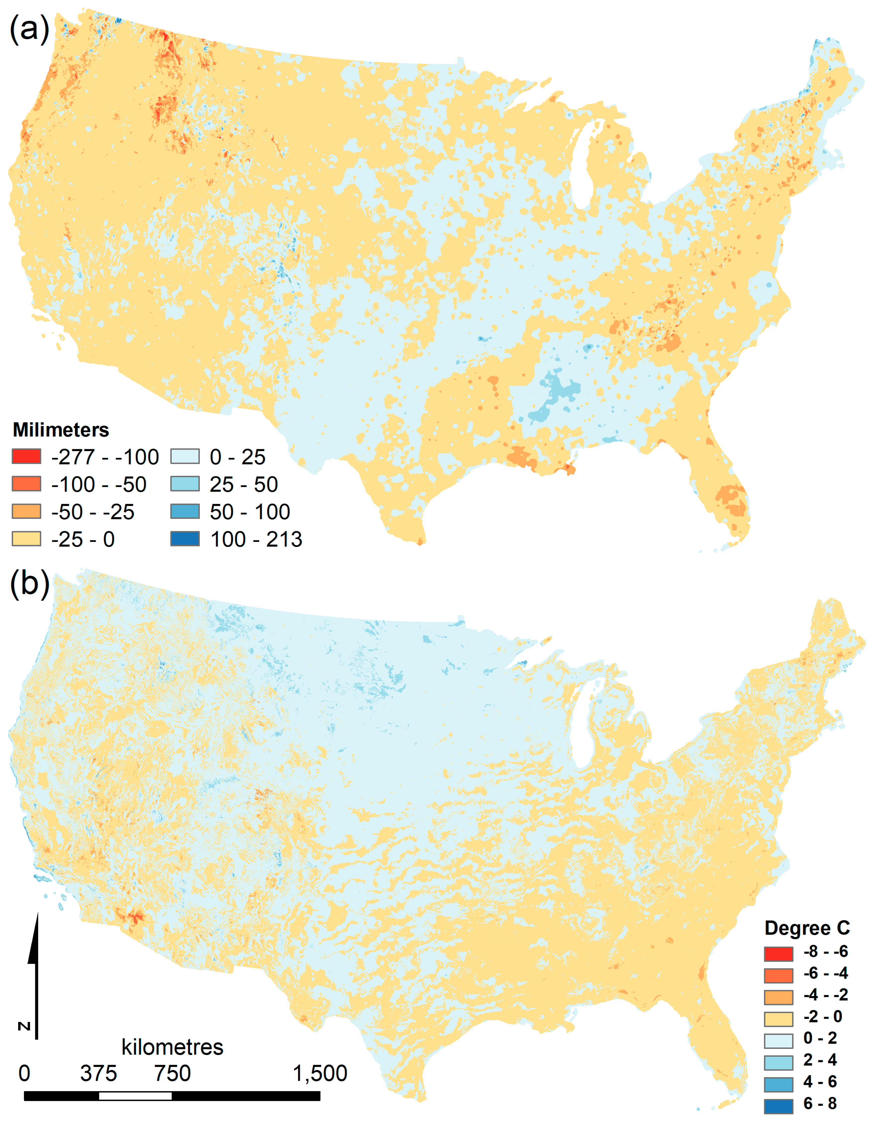
Climate averages over time are often described as climate “normals”, a standard mandated by the World Meteorological Organization, consisting of an arithmetic average of climate over a 30-year period and used as a reference point to compare to other time periods. The Parameter-elevation Regressions on Independent Slopes Model (PRISM) climate normals data set for the continental United States of America (USA) has been updated from monthly averages across 1971 to 2000 to include monthly averages across 1981 to 2010 [11]. Despite the overlap of two-thirds of the years, there are substantial changes in the 30-year average precipitation, maximum temperature, and minimum temperature. For example, parts of the USA exhibited over 200 mm more precipitation during the driest month in the earlier period while other regions had less precipitation at a comparable magnitude (Figure 1). Similar differences existed for minimum temperature of the coldest month, with spatial heterogeneity between areas that were colder or warmer between the two time periods.
In correlative models, model parameterization is dependent on the correlation structure between predictor variables and location data. Changes in correlation structure can be particularly important when extrapolating to novel climates [12], so understanding how correlations vary in space and time is important. If there is a temporal disconnect between location data collection and predictor variable coverage, and the predictor variable’s correlation structure is not constant through time, this could potentially have a large effect on model results.
The environmental data used to produce correlative species distribution models, including climate, are often based on what data are readily available rather than decisions made based on the research question or species of interest [8]. For example, the global WorldClim data set, which only provides climate normals (1950 and 2000 [13] or 1970 to 2000), was cited in 1950 of 6380 articles published between 2013 to 2017 (google scholar search including climate AND [“species distribution model” OR “niche model” OR “habitat suitability model” OR “environmental matching model”]). These results indicate that a high percentage of species distribution models used the readily available WorldClim data set rather than a data set with customizable time periods. The PRISM data set is commonly mentioned in papers focused in the USA (293 of 2720 articles included PRISM). Unlike WorldClim, this dataset is downloadable for two periods of climate normals and is available as monthly data that could be used to develop project-specific climate normals, albeit at a coarser spatial resolution. As readily available climate normals datasets continue to be used in species distribution models, it is important to assess the potential impact of the temporal period of climate data on model results.
Our objectives were to evaluate the sensitivity of correlative species distribution models to the choice of partially overlapping climate normals period, including variable importance, variable response curves, and prediction agreement, while also examining the consistency of the correlation structure between the two baseline data sets. We did this using readily available data and standard best practices for creating correlative models to mimic common applications of these models. We evaluated whether model results were more sensitive to a time period or model algorithm choice. We hypothesized that the effect of climate normals data would be less for a long-lived species (e.g., tree) than for a short-lived species (e.g., insect). In addition, we hypothesized that simpler model algorithms would be less sensitive to the choice of climate normals data time period. We investigated the sensitivity of species distribution models to climate time period used by creating models with species data for a variety of taxa with commonly used climate data that matched the 30-year time span recommended by the Intergovernmental Panel on Climate Change. We compared the uncertainty from baseline climate data to uncertainty from the model technique, one of the greatest sources of uncertainty from those quantified [14], and assessed the consistency of predictions.

2. Materials and Methods

2.1. Climate Normals

We used climate normals from two time periods, 1971 to 2000 and 1981 to 2010, from the PRISM climate group (http://www.prism.oregonstate.edu). These climate normals consisted of a 30-year average of monthly precipitation, maximum temperature, and minimum temperature for the coterminous USA at 800 m grain resolution. We derived 19 commonly used bioclimatic variables from these monthly climate normals using the methods of O’Donnell and Ignizio [15] that were derived from a previous version [13,16].

2.2. Species

We chose species covering a wide range of taxa that are believed to be climatically limited in their distribution. The species included Africanized honey bees (a genetic hybrid cross of Tanzanian Apis mellifera scutellata Lepeletier and a variety of European honey bee strains such as A. m. ligustica Spinola), ponderosa pine (Pinus ponderosa Douglas ex P. Lawson & C. Lawson), American pika (Ochotona princeps (Richardson, 1828)), Bachman’s sparrow (Peucaea aestivalis (Lichtenstein, 1823)), and kudzu (Pueraria lobata (Willd.) Ohwi.). Africanized honey bees spread into the USA starting in the 1990s, expanding northward from Brazil, and have a cold temperature constraint to their northern range boundary in the USA [17]. Ponderosa pine is a native tree species distributed mainly within the western USA and can be limited by soil moisture [18]. American pika are found discontinuously in mountainous areas in the western USA and cannot tolerate the high diurnal temperature often found at low elevations [19,20]. Bachman’s sparrow is an endemic species to the southeastern USA with northern populations migrating south in winter [21]. Kudzu is an invasive vine that has been present in the eastern USA since 1872 and has known sensitivity to cold temperatures, which is believed to control its northern range boundary [22].

2.3. Location Data

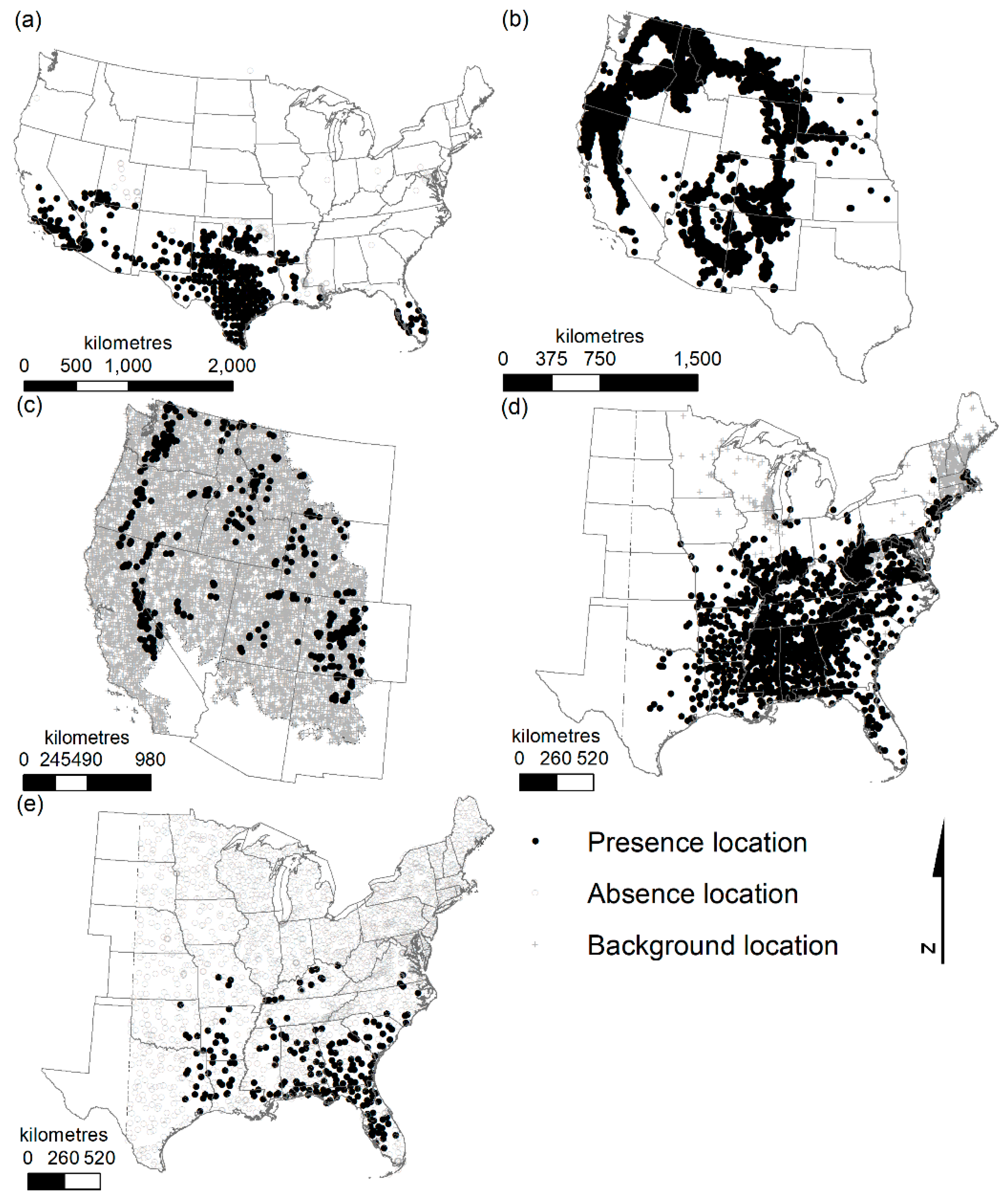
Occurrence data for each species were sourced from the best available and regionally appropriate data. When absence data had been collected, we used these for model development. Otherwise, we obtained background points attempting to match the sampling bias that existed in the presence points using the target-background approach [23]. Our study area was the continental USA, and we obtained available occurrence data for the entire area. We limited our area of inference (e.g., the area we produced mapped predictions for) to eastern or western states so we were not extrapolating to climate conditions outside the range of those included in model fitting. Species specific study areas are shown in Figure 2.
For Africanized honey bees, we used previously aggregated presence (n = 641) and absence (n = 107) data from Jarnevich et al. [24] (Figure 2a). The first record of Africanized honey bees in the USA occurred in 1990, so we did not limit the locations based on date.
Presence and absence data for ponderosa pine were obtained from the on-line Forestry Inventory and Analysis (FIA) data set, which consists of survey locations across the USA. The FIA program surveys 10 to 20 percent of all existing plots within a state on an annual basis, beginning in 1999 with historic periodic surveys by state from 1928 to 1999. The sample design consisted of a systematic grid of the USA of approximately 6000 acre hexagons, each containing a plot. All tree species are recorded on these plots. We selected surveys that occurred between 1979 and 2011 and, due to the large sample size, chose to subsample the data set spatially. Using the dismo library in R [25], we overlaid a 5 arc second grid onto the USA and randomly selected one location per grid cell, resulting in 5998 presence and 65,452 absence locations (Figure 2b).
We obtained 383 American pika presence locations from the Global Biodiversity Information Facility (GBIF; http://www.gbif.org; downloaded Oct 22, 2012), an organization that aggregates occurrence data primarily from museum records. We selected records with observation dates after 1970. We generated 10,000 background locations randomly within Landscape Conservation Cooperatives boundaries (LCC; http://www.fws.gov/landscape-conservation/lcc.html) containing American pika occurrences to characterize the available environment, as these boundaries are based on ecological characteristics (Figure 2c).
Bachman’s sparrow occurrences were obtained from North American Breeding Bird Survey (BBS) data (version 2011.0; https://www.pwrc.usgs.gov/bbs/). Any location that ever recorded a presence of Bachman’s sparrow between 1970 and 2006 was used as a presence location, and all other surveyed locations were classified as absence. To convert the BBS routes to point locations, we converted the shapefile of BBS routes to points using ArcGIS 10.0 (ESRI, Redlands, CA, USA) FeaturesToPoints tool. This method resulted in 196 presence locations and 2088 absence locations for Bachman’s sparrow within the study region (Figure 2e).
We obtained kudzu locations from the Early Detection and Distribution Mapping System (EDDMapS; http://www.eddmaps.org/) that contains presence locations of invasive species. We used the target background approach [23] to define background locations, selecting a similarly distributed non-native plant species with locations available in EDDMapS, Japanese knotweed (Fallopia japonica). Given their similarity, we assumed surveys for Japanese knotweed would have similar sampling bias. Many records did not include collection dates, but we removed any locations with a pre-1970 date. After removing these records and limiting to a single location within each 800 m cell within the eastern USA, we had 3427 presence locations and 2269 background locations (Figure 2d).

2.4. Analysis

We used the Software for Assisted Habitat Modeling (SAHM 1.2; [26]), a package in VisTrails [27] to perform the modeling analyses. To control for collinearity issues, we removed one of any pair of predictors with a maximum of the Pearson, Spearman, or Kendall correlation coefficients |r| >0.7 [28]. For correlated variable pairs, we retained the variable that was known through the literature to be a more important driver of the species distribution. We used four modeling algorithms common in species distribution modeling literature, including generalized linear models (GLM; [29]), multivariate adaptive regression splines (MARS; [30]), boosted regression trees (BRT; [31]), and random forest (RF; [32]). We used 10-fold cross-validation to evaluate individual model performance, and withheld 10% of the data for final evaluation across all models. SAHM provides standard assessment metrics including area under the receiver operating characteristic curve (AUC) and calibration plots [33,34].
We assessed consistency of variables retained in models and their importance to the model. GLM used stepwise selection based on Akaike’s information criterion; MARS used forward steps identifying many knots with backward pruning to simplify the model; and BRT only selected predictors for inclusion that minimized prediction errors. RF did not include an internal variable selection procedure. SAHM calculated variable importance consistently across model techniques using the change in AUC values when predictor values associated with training location data were permutated between presence and absence or background data. We transformed these importance values to relative percentages.
Consistency of predictions was assessed using discretized versions (i.e., binary maps) of the continuous output maps for each model with locations assigned to a suitable or unsuitable category. Results were discretized using the maximize sum of sensitivity and specificity threshold rule, which has performed well across data types [35]. We then summed the discretized maps by species, both across model algorithms to assess prediction differences due to climate data and across climate data to assess prediction differences due to model algorithms. For the former we calculated differences for all pairwise combinations to control for the effect of different sample sizes (four model algorithms compared to two time periods). We calculated the percent of each defined study area that had disagreement on suitable and unsuitable predictions to compare the differences caused by climate period and the differences caused by the model algorithm.
We also used SAHM to run pairwise correlations between the bioclimatic variables within the eastern, western, and continental USA for both climate normals periods. We randomly selected 10,000 points across each of the three regions to characterize climate. We used the maximum correlation coefficient of the Pearson, Spearman, and Kendall correlation coefficients to evaluate correlations among the bioclimatic variables. We then compared the correlation matrices between the two time periods to explore the temporal consistency of the correlation structure.

3. Results

All models performed well, with high cross-validation discrimination capacity (e.g., most independent split AUC values >0.9, all >0.8). Calibration plots also indicated good agreement between predicted probabilities of occurrence and observed occupancy, with a few exceptions (e.g., American pika and kudzu, which had background rather than absence data). However, for these analyses we were primarily concerned with discrimination ability.

3.1. Variable Correlation

Despite regional heterogeneity visible in the maps of differences in climate between the two climate normals periods (Figure 1), correlations between predictor variable values from 1971 to 2000 compared to the same predictor variable in 1981 to 2010 were similar (Table 1 and Table S1 diagonals). For all variables except mean temperature of the wettest quarter [bio8] in the eastern USA (Table S1b), correlations were |r| > 0.9. Mean temperature of the wettest quarter consistently had the lowest correlation, perhaps due to changes in the consecutive three-month period that comprised the quarter, as maps of this predictor are spatially disjointed.
Correlations between predictor variables within a single climate normals period also remained consistent when compared across climate normals periods (Table 1 mirror image above and below the diagonal). Differences in correlation coefficients for predictor variable pairs between the two time periods were commonly <0.05.

3.2. Variable Importance

Variable retention and importance ranking generally changed with a change in climate normals periods regardless of species or model algorithm (Table 2). While this was not the case for every pair of species and model type, each species and model type had at least one difference in variable retention or ranking. For kudzu, however, the only difference among models was that the 1971 to 2000 climate normals GLM model retained mean diurnal range, though with a very low relative importance value (0.1%; Table 2d). This predictor was dropped by the 1981 to 2010 climate normals GLM model. The other four variables were consistent between the GLM models in their order of importance. Africanized honey bee models also showed consistency in variable importance ranking among models with only one difference, where the third and fourth most important variables switched places in the RF model (Table 2a). Across model types maintaining a consistent climate period, each pairing had a difference in variable importance ranking or variable retention for three of five species.
Most differences among model pairings with a change in climate normals period involved a switch in the order of variable importance. In some cases variables were dropped during the model fitting process for one climate normals period while they were retained in the model fitting process using the other climate normals period. For example, the top two predictors in BRT models of Bachman’s sparrow were the same, but mean temperature of the wettest quarter was retained as a third predictor in the model using 1981 to 2010 climate normals data, but dropped from the model using 1971 to 2000 climate data (Table 2e). However, this predictor contributed relatively little to the model (6.1%).
Ponderosa pine and American pika, both modeled in the western USA, exhibited the greatest differences in variable importance between paired models from the two different time periods. These two species also had the greatest number of predictors retained after the variable selection correlation step (nine and eight, respectively, compared to five in the other species’ models).

3.3. Prediction Agreement

The choice of model algorithm generally caused greater differences in predictions between models than the choice of climate normals period (Table 3). The magnitude of differences in predictions between species, however, differed. Ponderosa pine had the largest difference in model algorithm choice (average of 16%), and American pika had the smallest (average of 3%). Africanized honey bees had the greatest difference related to selection of climate normals data (12.1% for the MARS models), and American pika, again, had the smallest difference (1.6% for both the GLM and RF models). However, American pika are relatively rare on the landscape. If we only consider areas predicted as suitable by at least one model, we have a much higher level of disagreement (1.6% to 4.9% compared to 14.0% to 40.7%).
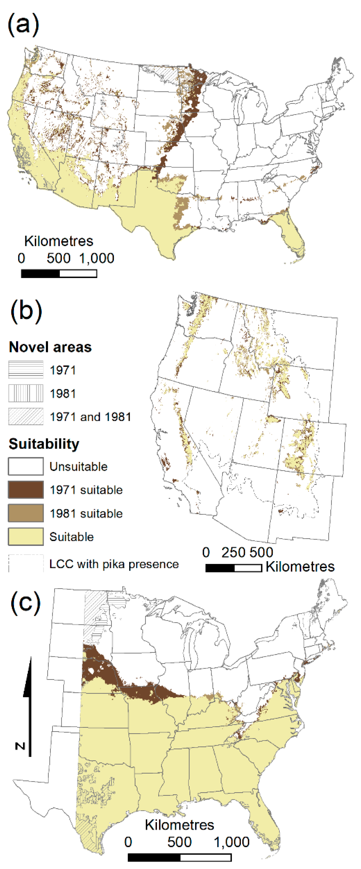
Most differences between model predictions, either from algorithm choice or climate normals period choice, occurred at the geographic edges of ranges, rather than within the interior of the predicted suitable habitat (Figure 3; Supplementary material Figure S1). For example, most of the disagreement between the choice of climate normals for kudzu was along the northern edge of the predicted suitable habitat (Figure 3c).
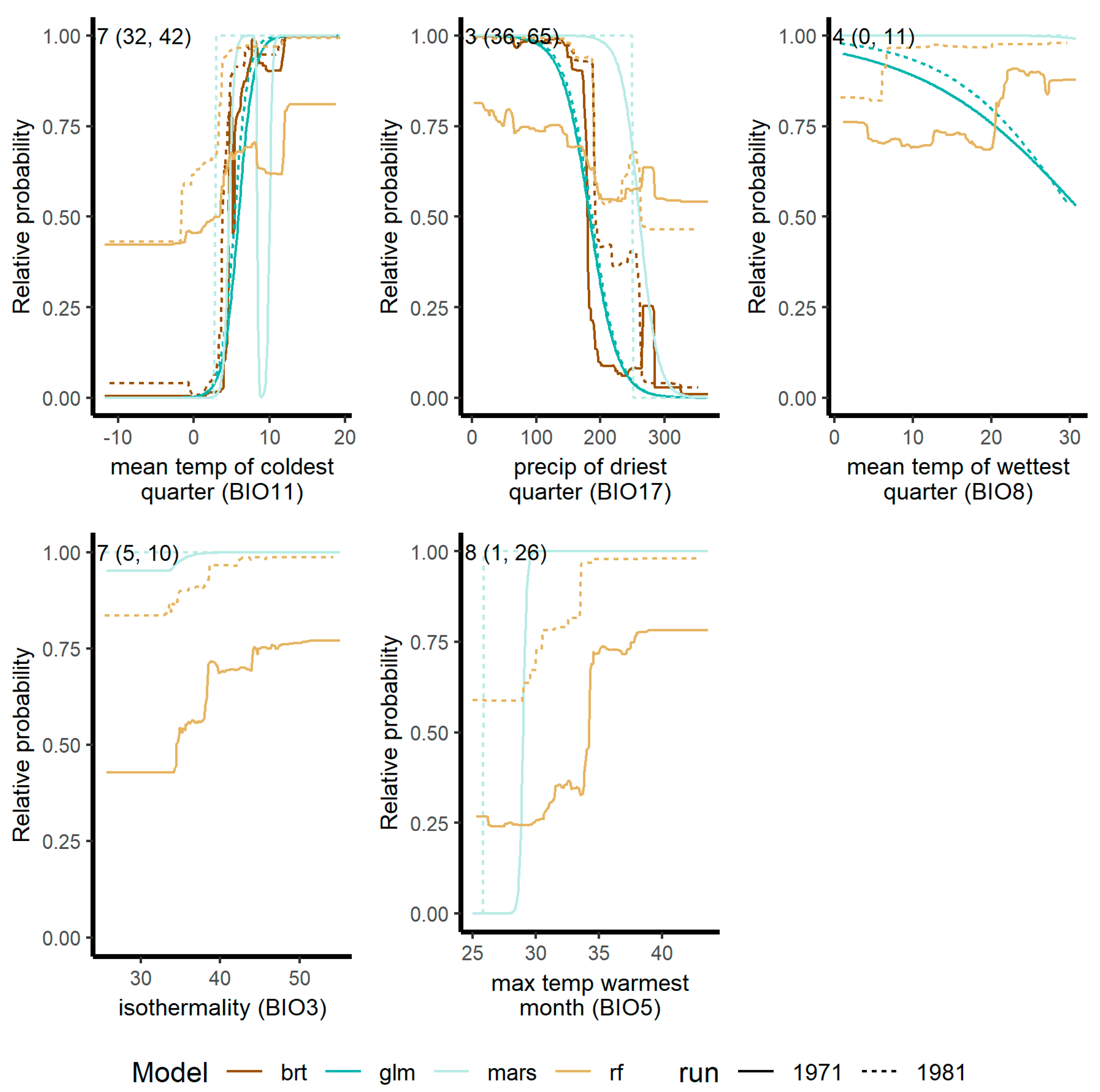
BRT models for Africanized honey bees for both time periods selected the same subset of predictors with similar levels of variable importance. However, the geographic predictions of suitability were still quite different (8.1% difference; Figure 3a) because the response curve shapes differed (Figure 4). All species had some differences in response curves (Supplemental information Figure S2).

4. Discussion

We found the choice of model algorithm had a larger effect on prediction results among models than did the choice of climate normals period, although the climate normals time period did affect model results. Our findings that choice of model algorithm contributed considerable uncertainty to model results are consistent with others [14,36]. This underscores the importance of evaluating multiple model algorithms when developing habitat suitability models [37]. There are several potential sources of uncertainty in species distribution modeling that have received attention in the literature [9,38,39,40,41,42,43], often focusing on quantifiable uncertainty. Some researchers have compared the relative contribution of different components of uncertainty to models [14,36]. These components range from quality of location data (e.g., misidentification or inaccurate coordinates) to variance arising from different modeling algorithms, finding that model algorithm choice contributed the greatest amount of uncertainty among the factors they examined. We also found that these differences were consistent across taxa, despite the differences in life history and occurrence information (e.g., availability of absence data) among species we tested.
Our results also complement those of others looking more specifically at climate data. Braunisch et al. [39] examined uncertainty introduced through the correlation filtering process to deal with collinearity between variables. Differences in predictions arose depending on the identity of the climate variables retained, similar to our findings of differences due to time period. In a similar study to this one, Roubicek et al. [44] tested the importance of a temporal mismatch between occurrence data and climate data, using different baseline climate data with simulated location data for 18 different 10-year time spans, one 30-year time span, and one 50-year time span. They highlighted the importance of a temporal match between species location data and climate time period. However, our study differs from previous work in that we use a larger spatial extent (US compared to East coast of Australia) and real applications, rather than simulated species, including a diverse group of taxa with differing lifespans and data qualities. In addition, Roubicek et al. [44] performed all modeling with Maxent, which is a presence–background technique, while we evaluate four commonly used techniques for presence–absence/pseudo–absence (but exclude Maxent as most modeled species had absence data). In this study we had temporal overlap between the two periods, with our location data generally spanning the climate normals periods covered. Our finding of model sensitivity to time period of climate normals is one aspect of uncertainty that was previously relatively unexplored.
Differences in variable importance and response curves due to the choice of climate normals time period resulted in measurable differences in predicted habitat suitability for the five species, even when only one-third of the data were different between the two periods. These differences arose despite the fact that values extracted from the two time periods were highly correlated (e.g., Table 1). If a subset of predictors was more highly correlated between the time periods, we could have tested if using the more correlated subset decreased differences between fitted models.
One use of correlative species distribution models istrying to predict shifting distributions due to climate change or range expansion of species [45,46,47,48]. As discussed elsewhere [49], correlative models have their limitations for these types of assessments. While model type produced greater variation than climate normals time period, the choice of time period did affect all species and all model algorithms tested. These impacts occurred regardless of species taxa, spatial extent (entire US or a subset), niche breadth (generalist such as ponderosa to specialist such as pika), and nativity, all of which can affect model performance. Our hypothesis that long-lived species would be less impacted did not hold up; in fact, Africanized honey bees had less change in predictor importance than ponderosa. These differences may only be exacerbated when applied to novel locations or time periods [50], as seen in other evaluations examining uncertainty [39].

5. Conclusions

We showed that even with species-tuned model parameters, rather than generic model parameterization that is often applied to large suites of species, results are highly sensitive to both baseline climate period and model method. While the latter is well recognized as an important uncertainty and is often accounted for through ensemble modeling [51], the impact of the former is not commonly assessed. We hypothesized that one particular modeling algorithm might consistently exhibit less impact, such as GLM because it is a simpler model with smoother response curves, but our results indicate that, instead, we have uncovered yet another source of uncertainty for model developers to evaluate on a case by case basis. Luckily, the development of somewhat automated software such as ModEco [52], BIOMOD [53] and VisTrails:SAHM [26] facilitate running multiple modeling algorithms several times to test the sensitivity of a model to a particular decision (e.g., choice of model algorithm, threshold rules, predictor data sets, background selection, etc.). Another possibility is that as the availability of climate data and computational processing capabilities increase, climate normals relative to time of sampling could be used (e.g., 30-year average prior to sampling year, or even a longer climate average spanning the range of sampling dates such as 1971–2010 in our case). Our results further highlight the uncertainty around using these types of correlative models for forecasting future distributions of species to inform conservation decisions. Evaluating uncertainty in current models is a necessary first step before determining if it is wise to proceed with projections.
Supplementary Materials

The following are available online at https://www.mdpi.com/2225-1154/7/3/37/s1, Figure S1. Habitat suitability maps for each species, Figure S2. Response curves by species, Table S1. Bioclimatic variable correlations.

Author Contributions

Conceptualization, C.J. and N.Y.; methodology, C.J. and N.Y.; software, C.J.; validation, C.J.; formal analysis, C.J. and N.Y.; investigation, C.J. and N.Y.; resources, C.J.; data curation, C.J.; writing—original draft preparation, C.J. and N.Y.; writing—review and editing, C.J. and N.Y.; visualization, C.J. and N.Y.; supervision, C.J.; project administration, C.J. and N.Y.; funding acquisition, C.J. and N.Y.

Funding

This research was funded by the U.S. Geological Survey Invasive Species Program.

Acknowledgments

Any use of trade, firm, or product names is for descriptive purposes only and does not imply endorsement by the U.S. government.

Conflicts of Interest

The authors declare no conflict of interest.

References

  1. Pearson, R.G.; Dawson, T.P.; Liu, C. Modelling species distributions in Britain: a hierarchical integration of climate and land-cover data. Ecography 2004, 27, 285–298. [Google Scholar] [CrossRef]
  2. Luoto, M.; Virkkala, R.; Heikkinen, R.K. The role of land cover in bioclimatic models depends on spatial resolution. Glob. Ecol. Biogeogr. 2007, 16, 34–42. [Google Scholar] [CrossRef]
  3. Barbet-Massin, M.; Jetz, W. A 40-year, continent-wide, multispecies assessment of relevant climate predictors for species distribution modelling. Divers. Distrib. 2014, 20, 1285–1295. [Google Scholar] [CrossRef]
  4. Briscoe, N.J.; Kearney, M.R.; Taylor, C.; Brendan, W.A. Unpacking the mechanisms captured by a correlative SDM to improve predictions of climate refugia. Glob. Chang. Biol. 2016, 22, 2425–2439. [Google Scholar] [CrossRef] [PubMed]
  5. Pacifici, M.; Foden, W.B.; Visconti, P.; Watson, J.E.M.; Butchart, S.H.M.; Kovacs, K.M.; Scheffers, B.R.; Hole, D.G.; Martin, T.G.; Akcakaya, H.R.; et al. Assessing species vulnerability to climate change. Nat. Clim. Chang. 2015, 5, 215–224. [Google Scholar] [CrossRef] [Green Version]
  6. Thomas, C.D.; Cameron, A.; Green, R.E.; Bakkenes, M.; Beaumont, L.J.; Collingham, Y.C.; Erasmus, B.F.N.; de Siqueira, M.F.; Grainger, A.; Hannah, L.; et al. Extinction risk from climate change. Nature 2004, 427, 145–148. [Google Scholar] [CrossRef] [PubMed] [Green Version]
  7. Rodda, G.H.; Jarnevich, C.S.; Reed, R.N. Challenges in identifying sites climatically matched to the native ranges of animal invaders. PLoS ONE 2011, 6, e14670. [Google Scholar] [CrossRef] [PubMed]
  8. Elith, J.; Leathwick, J.R. Species Distribution Models: Ecological Explanation and Prediction Across Space and Time. Annu. Rev. Ecol. Evol. Syst. 2009, 40, 677–697. [Google Scholar] [CrossRef]
  9. Jarnevich, C.S.; Stohlgren, T.J.; Kumar, S.; Morisette, J.T.; Holcombe, T.R. Caveats for correlative species distribution modeling. Ecol. Inform. 2015, 29 Pt 1, 6–15. [Google Scholar] [CrossRef]
  10. Soberon, J.; Peterson, A.T. Interpretation of models of fundamental ecological niches and species’ distributional areas. Biodivers. Inform. 2005, 2, 1–10. [Google Scholar] [CrossRef]
  11. PRISM Climate Group. Oregon State University. 2012. Available online: http://www.prism.oregonstate.edu/ (accessed on 14 February 2012).
  12. Elith, J.; Kearney, M.; Phillips, S. The art of modelling range-shifting species. Methods Ecol. Evol. 2010, 1, 330–342. [Google Scholar] [CrossRef] [Green Version]
  13. Hijmans, R.J.; Cameron, S.E.; Parra, J.L.; Jones, P.G.; Jarvis, A. Very high resolution interpolated climate surfaces for global land areas. Int. J. Climatol. 2005, 25, 1965–1978. [Google Scholar] [CrossRef] [Green Version]
  14. Dormann, C.F.; Purschke, O.; Márquez, J.R.G.; Lautenbach, S.; Schröder, B. Components of uncertainty in species distribution analysis: a case study of the Great Grey Shrike. Ecology 2008, 89, 3371–3386. [Google Scholar] [CrossRef] [PubMed]
  15. O’Donnell, M.S.; Ignizio, D.A. Bioclimatic Predictors for Supporting Ecological Applications in the Conterminous United States; U.S. Geological Survey Data Series 691; USGS: Reston, VA, USA, 2012.
  16. Nix, H. A biogeographic analysis of Australian elapid snakes. In Atlas of Elapid snakes of Australia; Longmore, R., Ed.; Australian Government Publishing Service: Canberra, Australia, 1986; pp. 4–15. [Google Scholar]
  17. Harrison, J.F.; Fewell, J.H.; Anderson, K.E.; Loper, G.M. Environmental physiology of the invasion of the Americas by Africanized honeybees. Integr. Comp. Biol. 2006, 46, 1110–1122. [Google Scholar] [CrossRef] [PubMed] [Green Version]
  18. Coops, N.C.; Waring, R.H.; Law, B.E. Assessing the past and future distribution and productivity of ponderosa pine in the Pacific Northwest using a process model, 3-PG. Ecol. Model. 2005, 183, 107–124. [Google Scholar] [CrossRef]
  19. Smith, A.T.; Weston, M.L. Ochotona princeps. Mamm. Species 1990, 1–8. [Google Scholar] [CrossRef]
  20. Millar, C.I.; Westfall, R.D. Distribution and climatic relationships of the American pika (Ochotona princeps) in the Sierra Nevada and western Great Basin, USA; periglacial landforms as refugia in warming climates. Arct. Antarct. Alp. Res. 2010, 42, 76–88. [Google Scholar] [CrossRef]
  21. Dunning, J.B. Bachman’s Sparrow (Peucaea aestivalis). In The Birds of North America Online; Poole, A., Ed.; Cornell Lab of Ornithology: Ithaca, NY, USA, 2006. [Google Scholar]
  22. Forseth, I.N.; Innis, A.F. Kudzu (Pueraria montana): History, Physiology, and Ecology Combine to Make a Major Ecosystem Threat. Crit. Rev. Plant. Sci. 2004, 23, 401–413. [Google Scholar] [CrossRef]
  23. Phillips, S.J.; Dudik, M.; Elith, J.; Graham, C.H.; Lehmann, A.; Leathwick, J.; Ferrier, S. Sample selection bias and presence-only distribution models: implications for background and pseudo-absence data. Ecol. Appl. 2009, 19, 181–197. [Google Scholar] [CrossRef] [PubMed] [Green Version]
  24. Jarnevich, C.S.; Esaias, W.E.; Ma, P.L.A.; Morisette, J.T.; Nickeson, J.E.; Stohlgren, T.J.; Holcombe, T.R.; Nightingale, J.M.; Wolfe, R.E.; Tan, B. Regional distribution models with lack of proximate predictors: Africanized honeybees expanding north. Divers. Distrib. 2014, 20, 193–201. [Google Scholar] [CrossRef]
  25. Hijmans, R.J.; Phillips, S.; Leathwick, J.; Elith, J. dismo: Species distribution modeling. R package version 0.8-11. 2013. Available online: http://CRAN.R-project.org/package=dismo (accessed on 19 August 2014).
  26. Morisette, J.T.; Jarnevich, C.S.; Holcombe, T.R.; Talbert, C.B.; Ignizio, D.; Talbert, M.K.; Silva, C.; Koop, D.; Swanson, A.; Young, N.E. VisTrails SAHM: visualization and workflow management for species habitat modeling. Ecography 2013, 36, 129–135. [Google Scholar] [CrossRef] [Green Version]
  27. Freire, J.; Silva, C.; Callahan, S.; Santos, E.; Scheidegger, C.; Vo, H. Managing Rapidly-Evolving Scientific Workflows Provenance and Annotation of Data. In International Provenance and Annotation Workshop 2006: Provenance and Annotation of Data; Moreau, L., Foster, I., Eds.; Springer: Berlin/Heidelberg, Germany, 2006; Volume 4145, pp. 10–18. [Google Scholar]
  28. Dormann, C.F.; Elith, J.; Bacher, S.; Buchmann, C.; Carl, G.; Carré, G.; Marquéz, J.R.G.; Gruber, B.; Lafourcade, B.; Leitão, P.J.; et al. Collinearity: a review of methods to deal with it and a simulation study evaluating their performance. Ecography 2013, 36, 027–046. [Google Scholar] [CrossRef]
  29. McCullagh, P.; Nelder, J.A. Generalized Linear Models, 2nd ed.; Chapman and Hall: London, UK; New York, NY, USA, 1989. [Google Scholar]
  30. Elith, J.; Leathwick, J. Predicting species distributions from museum and herbarium records using multiresponse models fitted with multivariate adaptive regression splines. Divers. Distrib. 2007, 13, 265–275. [Google Scholar] [CrossRef]
  31. Elith, J.; Leathwick, J.R.; Hastie, T. A working guide to boosted regression trees. J. Anim. Ecol. 2008, 77, 802–813. [Google Scholar] [CrossRef] [PubMed] [Green Version]
  32. Friedman, J.H. Greedy function approximation: A gradient boosting machine. Ann. Stat. 2001, 29, 1189–1232. [Google Scholar] [CrossRef]
  33. Pearce, J.; Ferrier, S. An evaluation of alternative algorithms for fitting species distribution models using logistic regression. Ecol. Model. 2000, 128, 127–147. [Google Scholar] [CrossRef]
  34. Phillips, S.; Elith, J. POC plots: Calibrating species distribution models with presence-only data. Ecology 2010, 91, 2476–2484. [Google Scholar] [CrossRef] [PubMed]
  35. Liu, C.R.; Berry, P.M.; Dawson, T.P.; Pearson, R.G. Selecting thresholds of occurrence in the prediction of species distributions. Ecography 2005, 28, 385–393. [Google Scholar] [CrossRef] [Green Version]
  36. Diniz-Filho, J.A.F.; Bini, L.M.; Rangel, T.F.; Loyola, R.D.; Hof, C.; Nogues-Bravo, D.; Araujo, M.B. Partitioning and mapping uncertainties in ensembles of forecasts of species turnover under climate change. Ecography 2009, 32, 897–906. [Google Scholar] [CrossRef]
  37. Qiao, H.; Soberón, J.; Peterson, A.T. No silver bullets in correlative ecological niche modelling: insights from testing among many potential algorithms for niche estimation. Methods Ecol. Evol. 2015, 6, 1126–1136. [Google Scholar] [CrossRef]
  38. Naimi, B.; Hamm, N.A.S.; Groen, T.A.; Skidmore, A.K.; Toxopeus, A.G. Where is positional uncertainty a problem for species distribution modelling? Ecography 2014, 37, 191–203. [Google Scholar] [CrossRef]
  39. Braunisch, V.; Coppes, J.; Arlettaz, R.; Suchant, R.; Schmid, H.; Bollmann, K. Selecting from correlated climate variables: a major source of uncertainty for predicting species distributions under climate change. Ecography 2013, 36, 971–983. [Google Scholar] [CrossRef]
  40. Beale, C.M.; Lennon, J.J. Incorporating uncertainty in predictive species distribution modelling. Philos. Trans. R. Soc. B Biol. Sci. 2012, 367, 247–258. [Google Scholar] [CrossRef] [PubMed]
  41. Synes, N.W.; Osborne, P.E. Choice of predictor variables as a source of uncertainty in continental-scale species distribution modelling under climate change. Glob. Ecol. Biogeogr. 2011, 20, 904–914. [Google Scholar] [CrossRef]
  42. Graham, C.H.; Elith, J.; Hijmans, R.J.; Guisan, A.; Peterson, A.T.; Loiselle, B.A. The influence of spatial errors in species occurrence data used in distribution models. J. Appl. Ecol. 2008, 45, 239–247. [Google Scholar] [CrossRef]
  43. Jarnevich, C.S.; Talbert, M.; Morisette, J.; Aldridge, C.; Brown, C.S.; Kumar, S.; Manier, D.; Talbert, C.; Holcombe, T. Minimizing effects of methodological decisions on interpretation and prediction in species distribution studies: An example with background selection. Ecol. Model. 2017, 363, 48–56. [Google Scholar] [CrossRef]
  44. Roubicek, A.J.; VanDerWal, J.; Beaumont, L.J.; Pitman, A.J.; Wilson, P.; Hughes, L. Does the choice of climate baseline matter in ecological niche modelling? Ecol. Model. 2010, 221, 2280–2286. [Google Scholar] [CrossRef]
  45. Keith, D.A.; Mahony, M.; Hines, H.; Elith, J.; Regan, T.J.; Baumgartner, J.B.; Hunter, D.; Heard, G.W.; Mitchell, N.J.; Parris, K.M.; et al. Detecting Extinction Risk from Climate Change by IUCN Red List Criteria. Conserv. Biol. 2014, 28, 810–819. [Google Scholar] [CrossRef] [PubMed]
  46. Huntley, B.; Collingham, Y.C.; Willis, S.G.; Green, R.E. Potential Impacts of Climatic Change on European Breeding Birds. PloS ONE 2008, 3, e1439. [Google Scholar] [CrossRef] [PubMed] [Green Version]
  47. Jarnevich, C.S.; Holcombe, T.R.; Bella, E.M.; Carlson, M.L.; Graziano, G.; Lamb, M.; Seefeldt, S.S.; Morrisette, J. Cross-scale assessment of potential habitat shifts in a rapidly changing climate. Invasive Plant. Sci. Manag. 2014, 7, 491–502. [Google Scholar] [CrossRef]
  48. Wakie, T.T.; Evangelista, P.H.; Jarnevich, C.S.; Laituri, M. Mapping Current and Potential Distribution of Non-Native Prosopis juliflora in the Afar Region of Ethiopia. PloS ONE 2014, 9, e112854. [Google Scholar] [CrossRef] [PubMed]
  49. Araújo, M.B.; Peterson, A.T. Uses and misuses of bioclimatic envelope modeling. Ecology 2012, 93, 1527–1539. [Google Scholar] [CrossRef] [PubMed] [Green Version]
  50. Baker, D.J.; Hartley, A.J.; Butchart, S.H.M.; Willis, S.G. Choice of baseline climate data impacts projected species’ responses to climate change. Glob. Chang. Biol. 2016, 22, 2392–2404. [Google Scholar] [CrossRef] [PubMed] [Green Version]
  51. Garcia, R.A.; Cabeza, M.; Altwegg, R.; Araújo, M.B. Do projections from bioclimatic envelope models and climate change metrics match? Glob. Ecol. Biogeogr. 2016, 25, 65–74. [Google Scholar] [CrossRef]
  52. Guo, Q.; Liu, Y. ModEco: an integrated software package for ecological niche modeling. Ecography 2010, 33, 637–642. [Google Scholar] [CrossRef] [Green Version]
  53. Thuiller, W.; Lafourcade, B.; Engler, R.; Araujo, M.B. BIOMOD—A platform for ensemble forecasting of species distributions. Ecography 2009, 32, 369–373. [Google Scholar] [CrossRef]
Figure 1. Change in climate normals between 1971 to 2000 and 1981 to 2010 for two bioclimatic variables including: (a) precipitation of the driest quarter (Bio17) (mm) and (b) minimum temperature of coldest month (Bio6) (°C) exhibiting regional heterogeneity.
Climate 07 00037 g001
Figure 2. Presence and absence (a,b,e) or background (c,d) data used to develop models for each species including: (a) Africanized honey bees, (b) ponderosa pine, (c) American pika (pseudo-absence locations), (d) kudzu (background locations), and (e) Bachman’s sparrow.
Climate 07 00037 g002
Figure 3. Agreement between models created using climate normals from 1971 to 2000 and 1981 to2010 for (a) the Africanized honey bee boosted regression tree models, (b) the American pika multivariate adaptive regression spline models, and (c) kudzu generalized linear models.
Climate 07 00037 g003
Figure 4. Response curves for the five predictors retained in the Africanized honey bee models including mean temperature of the coldest quarter, precipitation of the driest quarter, mean temperature of the wettest quarter, isothermality, and maximum temperature of the warmest month. Each graph includes response curves from the subset of the eight models retaining that predictor, including the four different model algorithms (boosted regression tree (BRT), generalized linear model (GLM), multivariate adaptive regression splines (MARS), random forest (RF) and the two different runs of each for the climate normal periods (1971 to 2000 and 1981 to 2010). The top left numbers in each graph are the average variable importance across all model with the range in parenthesis.
Climate 07 00037 g004
Table 1. Bioclimatic variable correlations across the USA for each variable between each climate normals period (1971 to 2000 as rows and 1981 to 2010 as columns) as the diagonal from top left to bottom right in bold. Correlations among climate variables within the 1971 to 2000 time period are below the diagonal and correlations among climate variables within the 1981 to 2010 time period are above the diagonal as a mirror image. Correlations are colored in a gradient from 1 as white to 0 as red to help visually determine if the top and bottom have similar correlations. Abbreviations are: annual mean temperature (bio1); mean diurnal range (bio2); isothermality (bio3); temperature seasonality (bio4); maximum temperature warmest month (bio5); minimum temperature coldest month (bio6); temperature annual range (bio7); mean temperature of wettest quarter (bio8); mean temperature of driest quarter (bio9); mean temperature of warmest quarter (bio10); mean temperature of coldest quarter (bio11); annual precipitation (bio12); precipitation of wettest month (bio13); precipitation of driest month (bio14); precipitation seasonality (bio15); precipitation of wettest quarter (bio16); precipitation of driest quarter (bio17); precipitation of warmest quarter (bio18); precipitation of coldest quarter (bio19).
1981bio1bio2bio3bio4bio5bio6bio7bio8bio9bio10bio11bio12bio13bio14bio15bio16bio17bio18bio19
1971
bio10.9980.1050.4990.5360.8650.9050.5220.4560.6370.9370.9480.2490.2610.3260.1870.2370.3270.2490.3
bio20.0940.9670.6410.1250.430.0230.360.0340.1580.0940.1550.6740.6440.5780.3350.660.5860.5530.521
bio30.5390.5740.980.810.4840.6420.5090.060.6370.2760.6840.2010.1780.2390.2220.2010.2190.3990.158
bio40.5420.0850.8350.9960.2970.8150.8980.1850.7610.2530.7730.2950.3290.2070.0960.320.2250.1680.55
bio50.8640.4120.4580.2620.990.6870.1560.4440.5240.9120.7740.1990.2450.0790.0380.2570.0790.0350.208
bio60.9050.040.680.8250.6610.9940.7950.1910.8020.7320.9820.3190.3090.3240.1810.2840.3350.1010.509
bio70.5340.3430.5790.9170.1480.8210.9850.140.6790.2860.7050.5670.5510.4370.3130.5510.4680.1540.775
bio80.4480.0430.0760.2210.4870.1740.1680.9270.2990.5870.2760.1060.150.1510.0220.1350.130.5220.324
bio90.6380.110.6660.7820.4790.8120.7210.2990.9680.4430.7730.1780.1230.2040.2170.1180.2220.2280.525
bio100.9310.1020.3020.2460.9230.7180.2770.6080.4260.9970.7920.2070.2260.2650.1680.2030.2580.3130.132
bio110.9460.1370.7240.7830.7550.9830.7330.2560.780.780.9980.2520.2440.2990.1570.2160.3060.1180.408
bio120.2670.660.120.3160.1790.3560.570.1040.220.2160.2770.9960.9410.8520.5370.9530.8760.7560.844
bio130.3020.6110.080.3460.220.3530.5480.1560.1720.2570.2840.9460.980.7030.3050.9940.7270.7140.862
bio140.3180.5990.1780.2390.090.3570.4730.1020.2390.2370.3030.8590.7180.9890.8290.7140.9930.780.704
bio150.1540.3820.2070.0920.0720.1870.3240.060.2040.120.1320.5350.3160.8230.9810.3260.8260.490.575
bio160.2670.6320.110.330.240.3190.5390.1320.1630.2220.2460.9560.9940.7240.330.9890.7370.7330.868
bio170.3220.6030.1470.2580.090.3690.4930.0740.2530.2330.3130.8740.7320.9920.830.7360.9940.7690.744
bio180.2530.5490.340.1510.0130.1250.1640.4990.2020.310.1210.7680.7210.7730.4880.7420.7510.9930.369
bio190.2990.5430.2010.5610.2360.5240.7810.3280.5350.1150.4080.8580.8780.730.5840.8850.7740.3940.995
Table 2. Variable importance for each model (modeling algorithm [Generalized linear model (GLM); Multivariate adaptive regression spline (MARS); Boosted regression trees (BRT); Random forest (RF)], and time period [1971 to 2000 (1971); 1981 to 2010 (1981)]) including those for (a) Africanized honey bee, (b) ponderosa pine, (c) American pika (pseudo-absence locations), (d) kudzu (target background locations), and (e) Bachman’s sparrow. The three most important predictors in each column are colored, with the darkest indicating most important and lightest third most important. Blanks indicate that the predictor was dropped from that model.
(a)GLMMARSBRTRF
19711981197119811971198119711981
Isothermality 6.810.0 5.85.0
Maximum temperature of warmest month 2.83.0 26.21.0
Mean temperature of wettest quarter0.23.49.010.9 0.00.0
Minimum temperature of coldest quarter39.632.036.937.641.837.931.936.6
Precipitation of driest quarter60.264.744.638.558.262.136.157.4
(b)GLMMARSBRTRF
19711981197119811971198119711981
Mean diurnal range12.714.9 0.20.2
Isothermality12.513.23.04.3 13.93.05.9
Maximum temperature of warmest month29.730.520.914.534.916.731.622.1
Minimum temperature of coldest month15.717.08.912.420.512.08.55.8
Mean temperature of wettest quarter13.59.833.932.418.214.615.715.7
Average annual precipitation1.10.930.331.026.434.829.841.4
Precipitation seasonality0.80.52.21.6 1.31.9
Precipitation of driest quarter8.08.2 8.02.72.2
Precipitation of warmest quarter6.05.00.83.8 7.14.8
(c)GLMMARSBRTRF
19711981197119811971198119711981
Mean diurnal range 9.0 4.27.07.6
Isothermality 22.8 3.33.6
Maximum temperature of warmest month100.0100.051.89.082.981.348.947.6
Minimum temperature of coldest month 5.037.9 8.09.7
Mean temperature of wettest quarter 0.52.85.33.88.86.9
Precipitation seasonality 3.8 4.64.8
Precipitation of warmest quarter 0.33.24.97.06.5
Precipitation of coldest quarter 11.050.04.85.912.513.4
(d)GLMMARSBRTRF
19711981197119811971198119711981
Average annual temperature72.166.792.294.393.194.076.083.7
Mean diurnal range0.1 1.01.16.96.04.43.1
Average annual precipitation18.324.04.33.3 14.77.4
Precipitation seasonality2.62.9 2.53.0
Precipitation of warmest quarter6.96.42.41.3 2.32.9
(e)GLMMARSBRTRF
19711981197119811971198119711981
Mean diurnal range15.923.615.25.7 16.48.8
Mean temperature of wettest quarter1.50.810.17.2 6.18.10.7
Minimum temperature of coldest quarter56.051.054.479.972.972.350.965.7
Precipitation seasonality15.27.4 1.00.6
Precipitation of wettest quarter11.517.220.37.327.121.623.724.2
Table 3. Percent of study area for each of the five species (Figure 2) considered where model predictions disagreed, calculated by comparing binary suitable/ unsuitable maps (a) across the two climate time periods (1971 to 2000 and 1981 to 2010) for each model algorithm, and (b) mean (minimum to maximum) percent for all six pairwise comparisons of the four different models (e.g., GLM compared to MARS, GLM compared to BRT) for the two climate time periods.
(a)Africanized honey beePonderosa pineAmerican pikaKudzuBachman’s sparrow
Generalized Linear Model (GLM)3.07.61.65.05.0
Multivariate Adaptive Regression Splines (MARS)12.15.64.93.64.0
Boosted Regression Trees (BRT)8.16.12.35.23.9
Random Forest (RF)5.44.71.64.38.6
(b)Africanized honey beePonderosa pineAmerican pikaKudzuBachman’s sparrow
1971–2000 climate12.6 (8.3–16.5)16.7 (5.3–25.0)3.7 (2.3–5.5)6.6 (4.1–9.7)6.4 (4.5–7.2)
1981–2010 climate10.0 (8.7–11.0)16.2 (4.4–23.4)3.6 (2.5–5.3)7.1 (4.9–9.0)8.2 (3.3–12.2)