Article

Observational Evidence of Neighborhood Scale Reductions in Air Temperature Associated with Increases in Roof Albedo

1
Civil and Environmental Engineering, University of Southern California, Los Angeles, CA 90089, USA
2
Heat Island Group, Lawrence Berkeley National Laboratory, Berkeley, CA 94720, USA
3
Altostratus, Inc., 940 Toulouse Way, Martinez, CA 94553, USA
*
Author to whom correspondence should be addressed.
Climate 2018, 6(4), 98; https://doi.org/10.3390/cli6040098
Submission received: 14 October 2018 / Revised: 17 November 2018 / Accepted: 23 November 2018 / Published: 12 December 2018
(This article belongs to the Special Issue Climate Change Resilience and Urban Sustainability)

Abstract

:
The effects of neighborhood-scale land use and land cover (LULC) properties on observed air temperatures are investigated in two regions within Los Angeles County: Central Los Angeles and the San Fernando Valley (SFV). LULC properties of particular interest in this study are albedo and tree fraction. High spatial density meteorological observations are obtained from 76 personal weather-stations. Observed air temperatures were then related to the spatial mean of each LULC parameter within a 500 m radius “neighborhood” of each weather station, using robust regression for each hour of July 2015. For the neighborhoods under investigation, increases in roof albedo are associated with decreases in air temperature, with the strongest sensitivities occurring in the afternoon. Air temperatures at 14:00–15:00 local daylight time are reduced by 0.31 °C and 0.49 °C per 1 MW increase in daily average solar power reflected from roofs per neighborhood in SFV and Central Los Angeles, respectively. Per 0.10 increase in neighborhood average albedo, daily average air temperatures were reduced by 0.25 °C and 1.84 °C. While roof albedo effects on air temperature seem to exceed tree fraction effects during the day in these two regions, increases in tree fraction are associated with reduced air temperatures at night.

1. Introduction

The urban heat island (UHI) effect describes a phenomenon whereby temperatures in cities are higher than their rural surroundings [1] and is the result of land transformations associated with urbanization, as well as increases in anthropogenic heat. The fraction of the world population that lives in urban areas was 54% in 2014 and is expected to rise to 66% by the year 2050 (WHO), suggesting that UHIs may affect more people in the future. Compounding UHIs is the fact that cities are facing increased warming due to the local impacts of global climate change; Sun et al. [2] found that areas in the greater Los Angeles region could see an increase of 60–90 extremely hot days per year by end of century under high emissions scenarios (RCP8.5: A scenario of comparatively high greenhouse gas emissions), posing threats to public and environmental health in addition to straining energy resources. While warming from climate change requires global action to mitigate, the UHI is a city-specific phenomenon with potential local solutions. UHI countermeasures, such as cool roofs and tree canopy cover, have been found in modeling studies to reduce urban temperatures when implemented at city scale [3]. Therefore, there are actions that cities can now take to mitigate UHIs, which will decrease the threat of future extreme heat dangers from climate warming. To design and implement appropriate countermeasures, cities need to characterize urban heat and its causes [4,5].
Urban heat islands (UHIs) are categorized as either (a) skin-surface UHIs (i.e., comparing urban and rural surface temperatures) or (b) air-temperature UHIs (i.e., comparing urban and rural air temperatures near the surface). Air-temperature UHIs are relevant to building energy use, thermal comfort, public health, pollutant emissions and formation, and climate, and as such, they are the focus of this study. While satellite observations can provide spatially extensive temperature observations, they are able to characterize only surface temperature and not air temperature; the other limitation with remote sensing is the coarse resolution of images, order tens to hundreds of meters, which results in homogenous measurements for small neighborhoods [6]. Thus, characterizing air temperatures relies on ground-based observations such as fixed weather stations or mobile transects.
Acquiring observations from fixed weather stations with sufficiently high spatial density to be representative at neighborhood-to-city scale is a major challenge in characterizing urban air temperatures. In addition, mobile transects can be useful for characterizing air temperatures for a neighborhood on a particular day, but characterizing large areas (e.g., entire cities) over temporal scales that are relevant for different meteorological regimes is prohibitive. UHI studies that rely on numerical weather prediction models can simulate both surface and air temperatures. While these models continue to resolve an increasing number of processes relevant to urban physics, it is helpful to conduct studies focused on air temperature UHIs using observations of the real world.
The UHI results in part from the transformation of natural land cover, including trees and vegetation, to pavements, buildings, and other elements of urban infrastructure [7]. Reductions in vegetation coverage can lead to decreases in evapotranspirative cooling, and thus increases in air temperatures in urban regions [8]. Man-made materials (e.g., asphalt concrete) used in roads and buildings usually have low albedo and high thermal inertia, leading to high absorption of shortwave solar radiation and high storage of thermal energy [9]. In addition, street canyons between buildings usually have low sky view factors, which can reduce longwave radiative losses from the city [9]. Other factors such as the size of the city [1], shading from buildings and trees [10], urban irrigation [11], changes in surface roughness length [12], and changes in anthropogenic heating [8] can also affect urban temperatures.
The UHI can be defined over a variety of spatial extents, ranging from neighborhood-scale to city-scale [13]. Most past studies have investigated UHIs at the city-scale by comparing temperatures of urban regions to surrounding rural areas [14,15]. Investigating the UHI in Los Angeles at the city-scale is tricky, as this metropolitan region is surrounded by ocean and mountains, and therefore, there is no obvious rural background for reference. Furthermore, there is a strong temperature gradient resulting from the onshore sea breeze [12,16], complicating the relationship between temperature and land use. Temperature variations within the Los Angeles region result from the superposition of effects from UHIs at multiple spatial scales and the sea breeze [16]. For this reason, this study focuses on investigating relationships between air temperature and land cover properties for clusters of neighborhoods within the Los Angeles area. Each cluster is small enough to make the effects of the sea breeze on temperature differences between stations negligible.
Past studies using satellite data, ground observations, and numerical modeling have highlighted the importance of albedo and green vegetation fraction in determining temperature differences between urban regions and rural surroundings. Utilizing global-scale satellite observations for 419 cities, Peng et al. [8] found that the daytime surface urban heat island intensity (SUHII) is related to urban-rural differences in vegetation cover, while the nighttime SUHII is associated with albedo and anthropogenic heat differences. Other satellite-based studies highlighted the correlation of SUHII with albedo and vegetation fraction for Rotterdam in the Netherlands [17] and 32 cities in China [14]. Sun et al. [2] used mobile transects and remote sensing to identify the important role of anthropogenic heat and vegetation cover on UHI formation in Phoenix during the winter season. Yan et al. [18] assessed the correlation between air temperatures measured by mobile transects and different land cover properties at the neighborhood-scale in Beijing and found that tree fraction at the scale of 20 m can explain most summertime temperature variations at noon. Model simulations from numerous studies have found that increasing albedo and vegetation cover can reduce urban peak surface and air temperatures [13,19]. Therefore, increasing urban albedo and vegetation fraction have been proposed as measures to reduce the urban heat island effect.
One of the contributing factors to the UHI effect is anthropogenic heating from air conditioning systems. Ohashi et al. [20] and Salamanca et al. [21] studied the effect of anthropogenic heating on the urban heat island effect in the Tokyo and Phoenix metropolitan areas, respectively. They found that the AC systems can contribute to the UHI effect up to 1–2 °C in Tokyo, and 1 °C in some urban parts of Phoenix, respectively.
Solar reflective “cool” surfaces (e.g., cool roofs, walls, and pavements) that increase urban albedo can decrease urban temperatures because they absorb less solar radiation than traditional dark surfaces, maintain cooler skin temperatures, and therefore transfer less heat into the atmosphere. Past modeling studies predict that adopting cool roofs can effectively reduce urban air temperatures in Los Angeles [12,22], Baltimore-Washington [23], New York [24], and other cities in the United States [13,25,26]. Zhang et al. [27] found an annual- and global-average reduction of 0.40 °C in the urban heat island effect due to increasing roof albedo globally from 0.15 to 0.90. Mohegh et al. [28] simulated the effect of cool pavement adoption and found that increasing pavement albedo by 0.40 can result in near-surface air temperature reductions in California cities ranging from 0.18 °C to 0.86 °C. Note that nearly all past studies investigating the influence of cool surface adoption on urban air temperatures are based on (1) results from computational models and (2) the assumption that cool surfaces are uniformly adopted citywide. In practice, cool surfaces may be adopted in a patchwork fashion at the neighborhood-scale. There is a lack of research using real-world observations to assess the influence of adopting cool surfaces on neighborhood temperatures. Using satellite observations, Mackey et al. [29] found stronger land surface temperature reductions induced by increasing urban albedo relative to increasing green vegetation in Chicago. However, the effectiveness of cool roofs in reducing near-surface air temperatures (as opposed to surface temperatures) still needs to be verified by observations in various cities.
To fill the aforementioned research gaps, in this study we investigate the influence of two important land cover properties (albedo and tree coverage) on neighborhood-scale near-surface air temperatures for two clusters of neighborhoods in the greater Los Angeles area. We use high spatial density meteorological observations to derive the sensitivity of air temperatures observed at each weather station to corresponding spatially aggregated albedo and tree coverage. In this way, we compute associations between air temperatures versus (a) albedo and (b) tree fraction.
Various state and city-level policies [30,31] have led to cool roof adoption on some commercial and residential buildings in Los Angeles, allowing us to analyze air temperature differences between neighborhoods with extensive use of cool roofs versus traditional dark roofs. The goals of this study are to provide observational evidence of the (a) relationships between neighborhood-scale air temperatures and land use and land cover (LULC) properties, and (b) the effectiveness of cooling strategies. To our knowledge, this is the first observational study to investigate associations between neighborhood-scale near-surface air temperatures and roof albedo.

2. Methodology

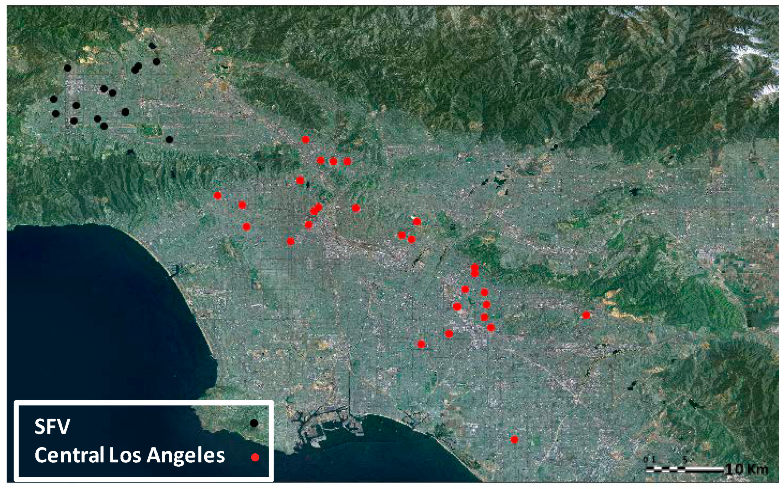
2.1. Areas of Analysis

The Los Angeles basin contains numerous microclimates leading to summer temperatures that range from moderate (at the coast) to hot (at the interior of the basin). The onshore sea breeze and distance from the coast play important roles in determining temperature variations within the basin. Land use and land cover properties also vary widely across the basin, with some regions consisting of primarily industrial/commercial land use, and others that are primarily residential. In this study, we have chosen two “regions” of interest within the Los Angeles Basin. Each region was chosen to fulfill two requirements: (1) It should be sufficiently small, such that distance from the coast does not dominate temperature variations; and (2) there should be sufficient variation in land cover properties of interest (e.g., roof albedo) to enable discerning effects of land cover on measured air temperatures. The first region encompasses an area of roughly 500 km2 and includes downtown Los Angeles; we refer to this region as Central Los Angeles. The second region encompasses roughly 160 km2 and is located within the San Fernando Valley (SFV). These two regions have distinctly different summertime baseline climates (Table 1). The monthly averaged daily minimum, maximum, and mean temperature is 19.4, 30.5, and 24.3 °C for SFV and 18.9, 27.7, and 22.5 °C for Central Los Angeles. Central Los Angeles typically experiences afternoon sea breezes, while SFV is largely unaffected by the influence of coastal air because of the Santa Monica mountains.

2.2. Defining Aggregation Areas

In this study, we aim to relate observed temperatures to LULC properties, in order to derive sensitivities of air temperature to aggregated existing LULC properties. We aggregate LULC properties (see Section 3.1) within a 500 m radius of each weather station (Figure 1). We expect that the LULC parameters in this aggregation area (referred to as a “neighborhood” from now on) can at least partially explain the variation in meteorological observations among the neighborhoods within each region. We are particularly interested in roof albedo as a LULC property to see whether observed temperatures are lower in neighborhoods that have roofs with higher albedo.

2.3. Meteorological Data

The meteorological data comes from a network of personal weather stations from Weather Underground [32]. We acquired all available meteorological parameters per station, including near-surface outside air temperature (referred to as “temperature” from now on), solar irradiance, air pressure, precipitation, relative humidity, wind speed, and wind direction for July 2015. This month was chosen because it was the latest data available at the time of acquisition. (June was intentionally avoided since Los Angeles generally experiences numerous cloudy days during that month.) Data from 76 stations were gathered within the two regions, but some stations did not measure certain meteorological parameters. Note that while we acquired all available parameters, we focused our analysis on temperature and solar irradiance. Figure 2 locates the weather stations and color codes them by region.
The data acquired from the network of personal weather stations, although provided with high spatial density, does not include quality control flags. We developed a three-step screening procedure to increase the quality of the meteorological dataset. In the first step, we removed values that were outside the range of observed minimum and maximum temperatures from the historical record reported by NOAA weather stations [33] across the LA Basin; corresponding minimum and maximum temperatures were −17 °C and 49 °C, determined using historical measurements in the domain for the past 130 years. Since the main focus of this study is to investigate urban temperature variability, in the second step we removed stations that were located in non-typical urban settings such as neighborhoods near golf courses or water reservoirs; the underlying drivers of land cover effects on local meteorology in these neighborhoods are likely different than neighborhoods with more typical urban cover. In the third step, stations with unphysical diurnal cycles were removed. Examples of unphysical diurnal cycles include having daily maximum temperatures at night (i.e., indicating a problem with the weather station timestamp), or diurnal temperature variations that were near zero (i.e., indicating a problem with the temperature sensor).

2.4. Description and Data Sources for Land Use Land Cover Properties

The land use land cover properties (referred to as “LULC” from this point on) are computed using data from multiple sources for each neighborhood.
Roof fraction ( f roof ) represents the ratio of building roof area (assumed equal to building footprint area) to neighborhood area. Roof fraction is computed using the Los Angeles Region Imagery Acquisition Consortium (LARIAC) dataset shapefiles for building footprints [34].
Tree fraction ( f tree ) is computed using a tree dataset from LARIAC with a spatial resolution of 4′ (1.2 m). This dataset is binary, indicating whether or not each pixel has tree cover. Analogous to roof fraction, the tree fraction represents the ratio of tree covered area to neighborhood area.
Pavement fraction ( f pavement ) represents the area fraction of pavement per neighborhood, with pavement area contributions from parking lots and paved roadways. Parking lot area is computed using parking lot boundaries given by LARIAC dataset shapefiles. Paved street area is derived using a street centerline dataset [35]. The total roadway length is computed by summing roadway length per neighborhood, and roadway area is then calculated by multiplying by an assumed roadway width of 12.8 m. Note that this roadway width represents the average street plus sidewalk width for Los Angeles, calculated using the weighted mean roadway width per building type [36], where the weighting factor is determined using the relative quantity of different building types in LA.
Reflected solar power from roofs ( P roof ) represents the average daily solar power (W) reflected from roofs within the neighborhood. This is computed as:
P roof = I × α roof × f roof × A
where I is the average daily incoming solar power (W m−2), α roof is the weighted average roof albedo in the neighborhood, and A is the neighborhood area (π × (500)2 m2 = 7.85 × 10⁵ m2) (see the next section for more information on the neighborhood areas). The average daily solar power of the day includes all 24 hours, not just sunlit hours. The area-weighted mean roof albedo ( α roof ) is determined using a dataset for seven California cities that reports building-specific roof albedos using remote sensing data [37]; the mean roof albedo is computed for each neighborhood using the roof’s area as the weighting factor. Overall, the metric P roof is used to account for the influence of cool roofs, considering (a) the mean roof albedo of the neighborhood, (b) the spatial coverage of roofs in the neighborhood, and (c) the daily solar irradiance. This avoids biases that could occur when, for example, the mean roof albedo of a neighborhood may be high, but spatial coverage of roofs is low.
Reflected solar power from neighborhood ( P neighborhood ) represents the average daily solar power (W) reflected from the entire neighborhood. This parameter is estimated as:
P neighborhood = I × α neighborhood × A
where α neighborhood is the average albedo of the neighborhood. The average neighborhood albedo is estimated using Equation (3), assuming that the neighborhood is comprised of roofs, pavements, and trees:
α neighborhood = α roof × f roof + α pavement × f pavement + α tree × f tree f roof + f tree + f pavement
Note that this formula does not consider the interaction between walls and pavements in the canopy. Since spatial datasets describing pavement and tree albedos do not exist, we assume values of 0.10 and 0.15, respectively. Due to potential inaccuracies in the GIS datasets, and because neighborhoods can consist of surface types other than roofs, pavements, and trees, f roof + f tree + f pavement generally does not equal 100%. Thus, the denominator of Equation (3) ensures that neighborhood-to-neighborhood variability in f roof + f tree + f pavement does not lead to variability in neighborhood albedo. While this calculation provides a relatively crude estimate of reflected solar power from the neighborhood, it is sufficient for the purposes of our study since this metric is used only for supporting analysis.
Reflected solar power from non-roof surfaces ( P non roof ) represents the average daily solar power (W) reflected from surfaces other than roofs in the neighborhood. This parameter is computed as P neighborhood P roof .
Other LULC properties: Several other LULC properties were found to have insignificant associations with neighborhood scale temperatures. Thus, they are described only briefly here and are addressed further in the Supplemental Material. Impervious fraction is calculated as the sum of roof and pavement fraction. Building height is the mean height (weighted by footprint area) of buildings in a neighborhood and is acquired from the LARIAC dataset. Overall albedo (i.e., albedo accounting for all surfaces) is calculated as presented in Equation (3).

2.5. Deriving Sensitivities of Measured Air Temperature to LULC Properties

We compute sensitivity as the linear regression of temperature to LULC properties within a region (i.e., SFV or Central Los Angeles) for each hour of every day in July 2015 (i.e., 24 × 31 = 744 regressions per LULC property). Note that times reported in this study represent hourly averages (e.g., values reported for hour of day 15 actually represent the hourly average from 14:00–15:00, and all values are reported in local daylight time (LDT). Thus, each regression looks at temperature versus land cover variability from station to station within a given region. Figure 3 shows how the sensitivity of temperature to a LULC property (e.g., reflected solar power from roofs) is calculated for an example hour of the day, 14:00–15:00 LDT. Each point on the figure represents an hourly average value of temperature and spatially aggregated LULC property associated with one weather station. After a multi-step outlier removal process (explained in the next paragraph), the sensitivity of the temperature to the LULC property is calculated. We perform these regressions for each hour of the day and thus acquire hourly sensitivities for the entire month of July 2015. Investigating sensitivities for each hour of the day can help hypothesize physical processes that are driving the observed correlations. We only compute these regressions for sunny days, defined as those with daily maximum solar irradiance >700 W m−2.
To ensure that regression results are not dominated by a small number of weather stations, we take the following steps to remove outlying data:
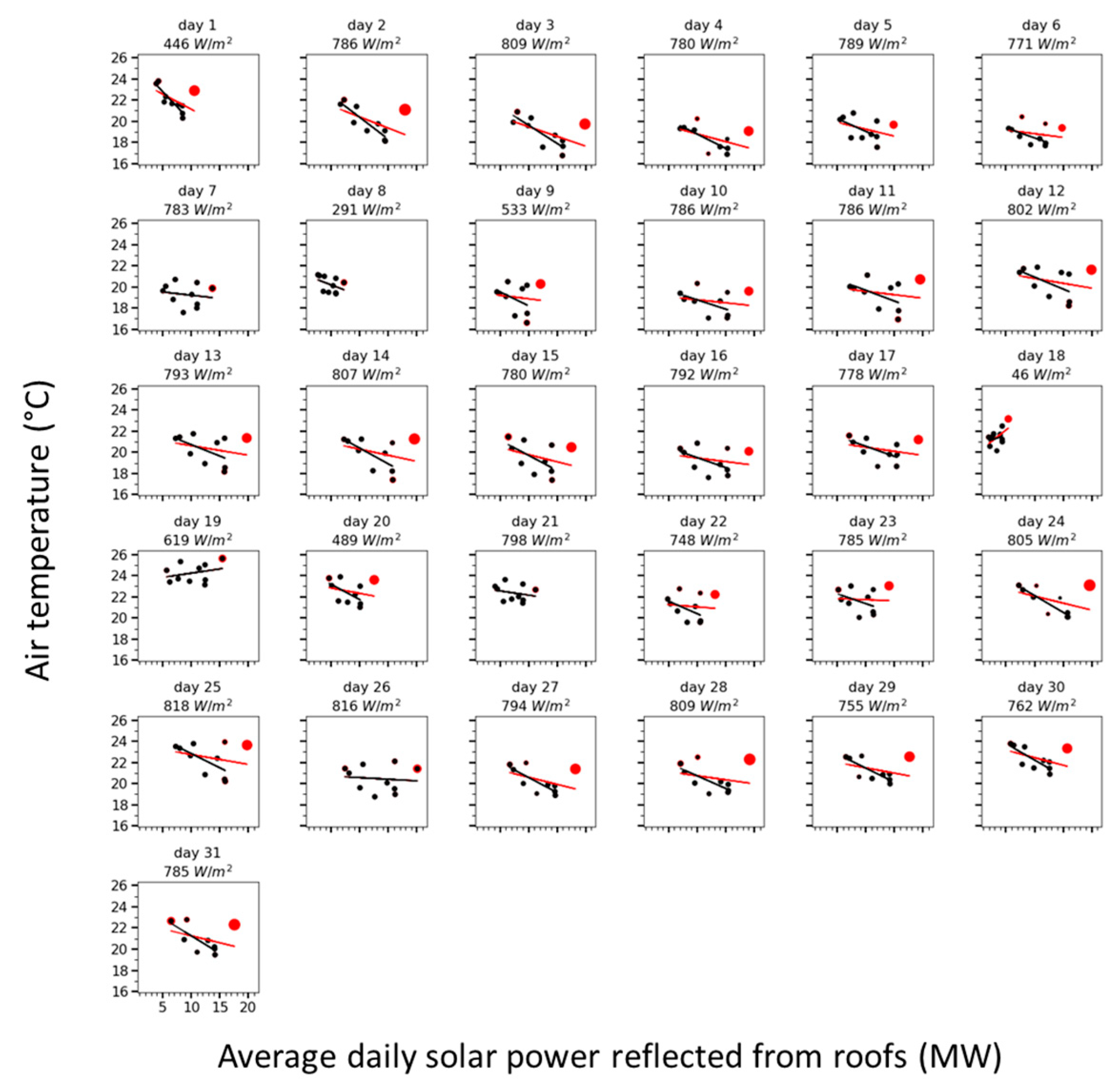
  • We first detect and remove outlier weather stations for each hour. This is carried out by first performing a standard least squares linear regression. The influence of each point in determining the regression slope is then computed using leverage and residuals. Based on the distribution of influences for each hour and region, data points that have influence beyond 1.5 times the inner quartile range of the distribution are removed. This tends to eliminate points that have too much influence in determining the final regression statistics. After these points are removed, another regression is carried out. This time we use a robust linear regression with a Huber-T objective function [38]. Regression using the Huber objective function gives higher weights to points with lower residuals, whereas standard regression using least-squares gives equal weights to each observation. The combination of outlier removal and robust regression minimizes the role of observations with high leverage, high residuals, or both. The sensitivity of temperature to the LULC parameter x is then computed as the slope of the robust regression (i.e., Δ T Δ x ).
  • Next, we determine whether the computed spatial sensitivity is statistically distinguishable from zero. We do so by computing the probability (“p”) value of the aforementioned robust regression. We deem the hourly sensitivity significant if the p-value is less than 0.1. The choice of this value was rather subjective.
  • Lastly, for each hour of the day, we compute the number of days in July with statistically distinguishable sensitivities for each land cover property. Those sensitivities with >10 significant days are deemed as having significant relationships for that hour of the day. Those with ≤10 are deemed insignificant. This threshold was chosen subjectively, but roughly corresponds to half the number of sunny days for this month.

3. Results

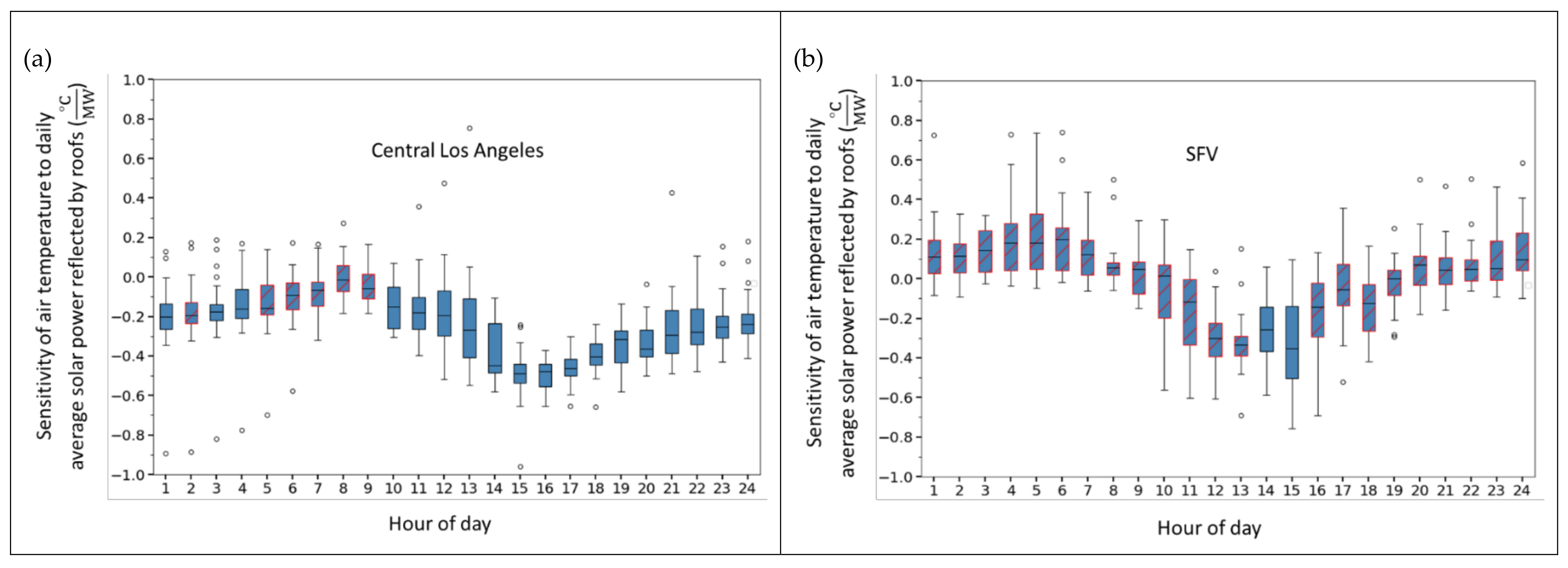
3.1. The Sensitivity of Temperature to Solar Power Reflected from Roofs

Panels a and b of Figure 4 present sensitivities of temperature to daily average solar power reflected by roofs for Central Los Angeles and SFV, respectively. Note that sensitivities for morning hours before sunrise use the average solar power of the previous day in Figure 4. Each box and whisker set shows the distribution of values for sensitivity per hour over all sunny days (daily maximum solar irradiance >700 W/m²) in July 2015.
Median sensitivities for Central Los Angeles (Figure 4a) are negative at all times of day, with most hours exhibiting statistically significant values. The largest negative sensitivity (0.49 °C per 1 MW increase in daily average solar power reflected) occurs at 14:00–15:00 LDT, which is consistent with the hottest time of day in this region (Figure S1). This matches our expectation based on the underlying physical processes involved since cooling occurs via increases in reflected solar radiation. While reflected solar radiation peaks at 13:00 LDT, there is an apparent lag between maximum radiation and maximum cooling. As the sun sets, sensitivities trend toward zero, and reach the lowest (negative) sensitivity right before sunrise. This again matches our expectation based on physical mechanisms since temperature reductions induced by increasing reflected solar radiation are expected to diminish after the sun goes down. The observed lag between peak temperature reduction and peak solar irradiance and the non-zero sensitivities at night are likely caused by the thermal inertia of roofs. Note that in Los Angeles, the peak temperature occurs earlier than in many other cities that do not experience an afternoon sea breeze.
Sensitivities of temperature to daily average solar power reflected by roofs for SFV (Figure 4b) show a similar diurnal shape as that of Central Los Angeles. However, most hours of the day have sensitivity values that are not statistically significant in SFV. Sensitivities at 13:00–14:00 and 14:00–15:00 LDT are significant, however. While sensitivities for some hours of the night are positive, indicating counterintuitively that temperatures are positively correlated with increased daily reflected solar power, these values are not statistically significant. At 14:00–15:00, sensitivities are 0.31 °C per 1 MW increase in daily average solar power reflected from roofs.

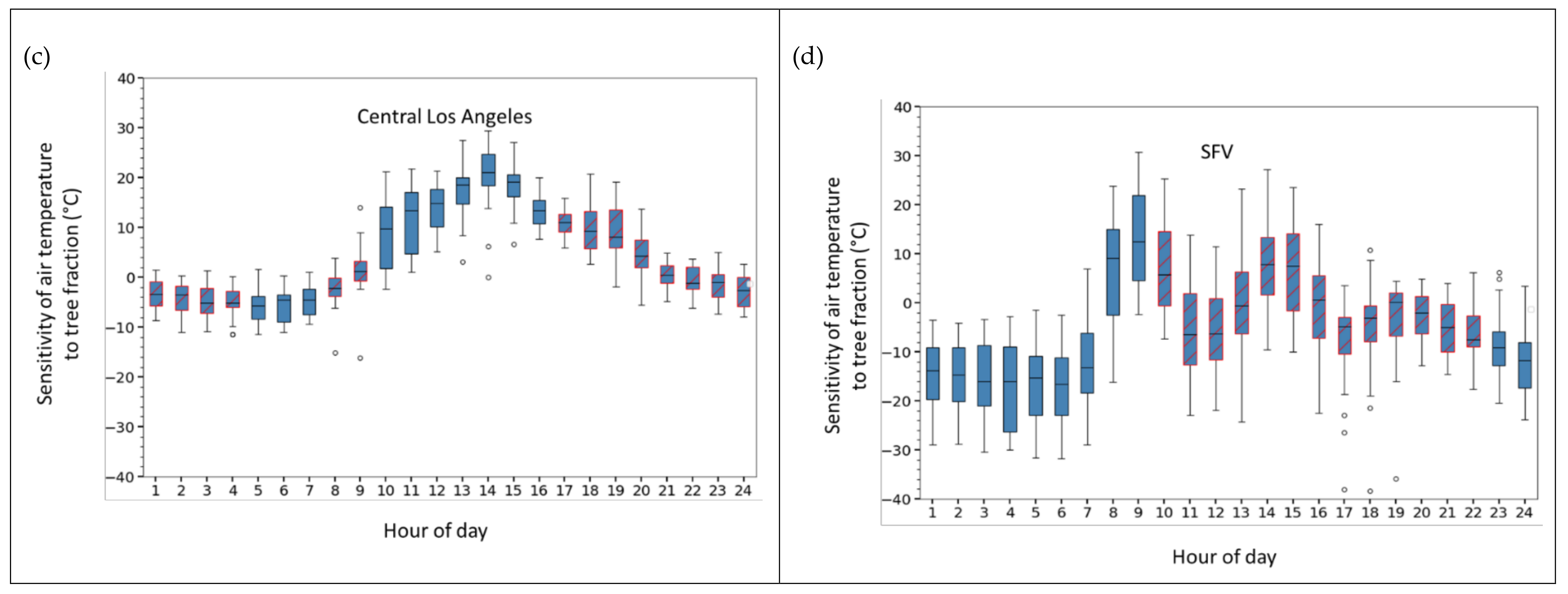
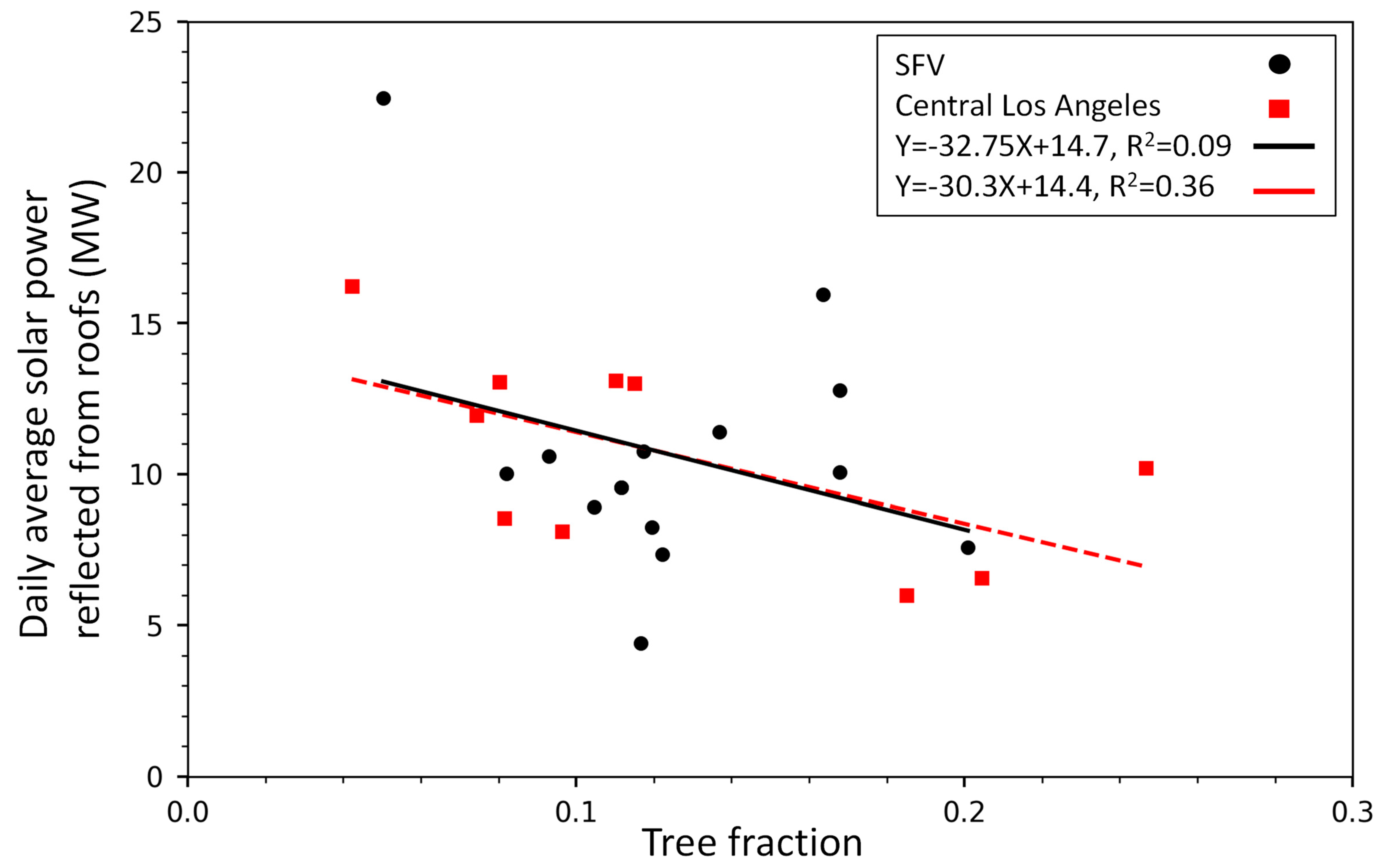
3.2. The Sensitivity of Temperature to Tree Fraction

Panels c and d of Figure 4 present sensitivities of temperature to tree fraction for Central Los Angeles and SFV, respectively. In Central Los Angeles, these sensitivities are positive for most sunlit hours of the day, and negative at night. The maximum positive sensitivity is observed in the early afternoon (13:00–14:00 LDT). The apparent positive sensitivities during daytime counter expectations based on the underlying physical mechanisms since increased tree cover should be associated with temperature reductions through increased evaporative cooling and shading of surfaces. We suggest that these positive daytime sensitivities are actually driven by co-variations between temperature, tree fraction, and daily average reflected power from roofs.
To investigate this hypothesis, we present daily average solar power reflected from roofs versus tree fraction for each neighborhood (Figure 5). Solar power reflected from roofs is anti-correlated to tree fraction, with a coefficient of determination of 0.36 for Central Los Angeles. This is consistent with our assertion that solar power reflected from roofs drives temperature reductions (and apparent positive sensitivities between temperature and tree fraction) since (a) neighborhoods with lower tree fraction are associated with higher solar power reflected from roofs and lower temperatures; and (b) the underlying physical mechanisms suggest that increases in solar power reflected from roofs should lead to temperature reductions, while increases in tree fraction should not lead to temperature increases. Additional evidence for this assertion is that the diurnal cycles for the sensitivity of temperature to (a) daily average solar power reflected from roofs (Figure 4a) versus (b) tree fraction (Figure 4c) nearly mirror each other. The largest negative and positive sensitivity values occur in the early afternoon in both Figure 4a,c, respectively. To summarize, we assert that daily average solar power reflected from roofs is likely driving both observed temperature reductions and the apparent positive association between temperature and tree fraction in this region. This suggests that variations in solar power reflected from roofs (and thus roof albedo) appear to dominate variations in observed air temperature relative to the effects of tree fractions in Central Los Angeles.
For SFV, sensitivities of temperature to tree fraction are mostly statistically insignificant, though some values are significant during nighttime. These significant nighttime values are negative, suggesting that increased tree fraction is associated with temperature reductions, as expected based on the underlying physical mechanisms. Observations suggest a temperature reduction of up to about 1.5 °C per 0.1 increase in tree fraction at night (hours 00:00–7:00 LDT). We do not observe significant positive sensitivity during the day in SFV, as was observed for Central Los Angeles. We suggest that this is because solar power reflected by roofs has lower correlation with tree fraction in SFV ( R 2 = 0.09 ) than in Central Los Angeles ( R 2 = 0.36 ). The reduced coefficient of determination would lead to less co-variation among temperature, solar power reflected from roofs, and tree fraction.
We note that the sensitivities reported above are likely specific to the region under investigation. Other regions with different baseline (a) tree coverage, (b) tree physical properties, (c) soil moisture, and (d) meteorology, among other factors, are likely to show different relationships between air temperature and tree fraction.
Sensitivities of temperature to other LULC properties are presented in Figures S2–S4.

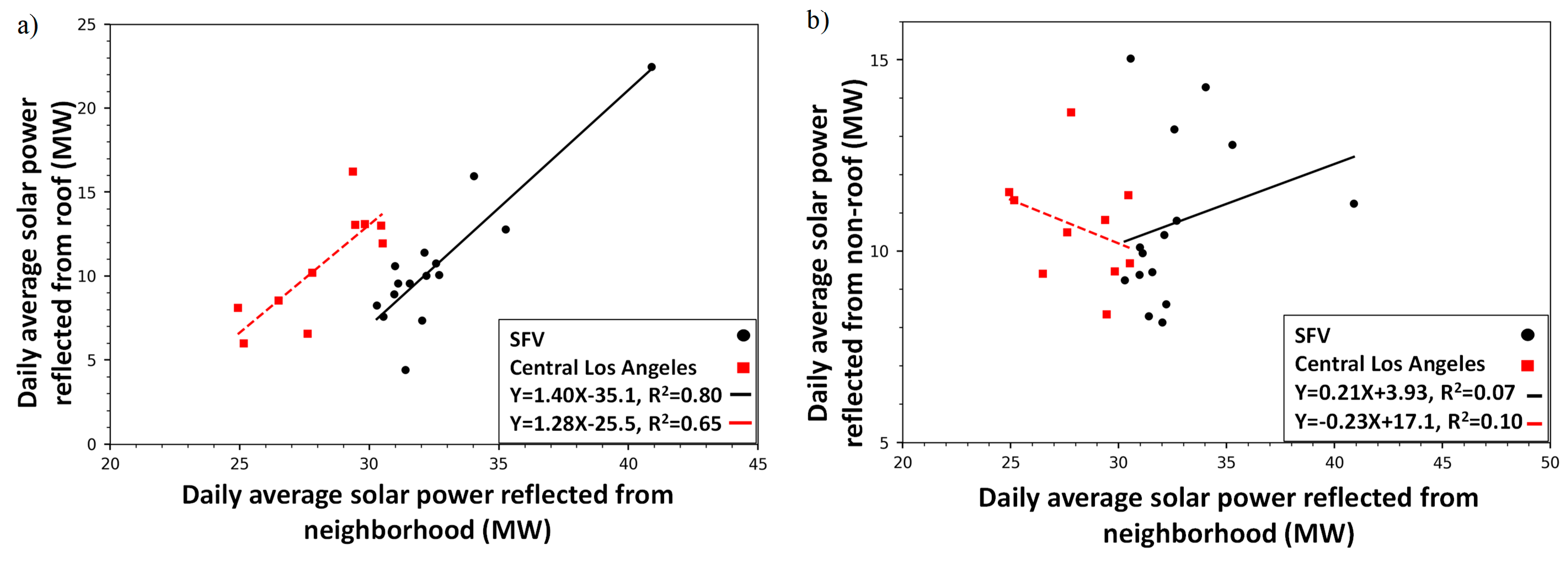
3.3. Roof versus Non-Roof Surfaces as Contributors to Variability in Solar Power Reflected from Neighborhoods

Here we test whether or not apparent temperature reductions associated with increases in solar power reflected by roofs are driven by co-variations in solar power reflected by non-roof surfaces, such as vegetation and pavement. To do so, we first present the daily average solar power reflected from roofs versus solar power reflected from the neighborhood (Figure 6a). In this analysis, each point represents a different neighborhood. High values of coefficient of determination (R2 = 0.80 in SFV and 0.65 in Central Los Angeles) indicate that a large proportion of the variance in solar power reflected from the neighborhood is explainable through variations in solar power reflected from roofs. In Figure 6b, we present the daily average reflected solar power from non-roof surfaces versus solar power reflected from the neighborhood. In this case, coefficients of determination are much lower (R2 = 0.07 in SFV and 0.10 in Central Los Angeles). This suggests that variations in daily average solar power reflected from the neighborhood are dominated by variations in solar power reflected by roofs rather than non-roof surfaces. This provides additional evidence that observed temperature reductions are driven by increases in solar power reflected by roofs in these regions.

4. Discussion

4.1. Comparison with Literature

In this section, we report sensitivities of air temperature to roof and overall albedos from our study and compare them to previous work. All relevant values are summarized in Table 2.
In our study, values for mean daily temperature reductions are 0.25 °C and 1.84 °C per 0.1 increase in roof albedo for SFV and Central Los Angeles, respectively, although the sensitivity for SFV is statistically insignificant. Note that the hottest time of day in the regions under investigation is 14:00–15:00 in Central Los Angeles and 16:00–17:00 LDT in SFV (Figure S1). We can also convert the sensitivities of air temperature to roof albedo ( Δ T Δ α roof ) derived in the current study to the sensitivities to overall albedo ( Δ T Δ α neighborhood ) using the computed average roof fractions of 26% and 28% for SFV and Central Los Angeles (values are calculated for neighborhoods that are not outliers), respectively, as:
Δ T Δ α neighborhood = Δ T Δ α roof × 1 f roof
Computed daily average air temperature reductions are 0.96 °C and 6.56 °C per neighborhood albedo increase of 0.1 for SFV and Central Los Angeles, respectively.
Santamouris [3] reviewed past modeling work on urban heat mitigation strategies. Most previous modeling studies reviewed in that paper had investigated the simulated temperature reductions attainable through hypothetical city-wide adoption of reflective surfaces. Santamouris [3] reported daily average air temperature reductions of 0.2 °C per 0.1 increase in roof albedo, and reductions in peak temperature of 0.4 °C per 0.1 increase in roof albedo. Per 0.1 increase in overall albedo, the average and peak temperature reductions were 0.3 °C and 0.9 °C, respectively.
In a more recent study, Vahmani et al. [12] investigated the effects of city-wide adoption of cool roofs on near-surface air temperatures in southern California. They found near-surface air temperature reductions of 0.9 °C at 15:00 LDT per increase of 0.26 in roof albedo. (Note that climate model results are generally reported as local standard time (LST). Modeling results from other studies are converted here to LDT for consistency with our observational results. In addition, model results are generally reported as snapshots of the reported time rather than hourly averages. Thus, we report exact times rather than hourly ranges for modeling studies.) This translates to air temperature reductions of 0.35 °C per 0.1 increase in roof albedo, and 1.84 °C per 0.1 increase in overall albedo. Zhang et al. [22] investigated the influence of city-wide adoption of cool roofs (and also cool walls) on canyon air temperatures in Los Angeles County. They found that adopting cool roofs led to decreases of 0.72 °C at 15:00 LDT and 0.48 °C in daily average temperature per increase of 0.8 in roof albedo. These sensitivities translate to canopy air temperature reductions at 15:00 LDT of 0.09 °C per 0.1 increase in roof albedo, and 1.03 °C per 0.1 increase in overall albedo, and daily temperature reductions of 0.06 °C per 0.1 increase in roof albedo, and 0.34 °C per 0.1 increase in overall albedo. In our study, air temperature reductions at 14:00–15:00 LDT are 0.05 °C and 5.5 °C per 0.1 increase in roof albedo for SFV and Central Los Angeles, respectively. These sensitivities translate to 0.19 °C and 19.7 °C air temperature reductions at 14:00–15:00 LDT per 0.1 increase in overall albedo.
Perhaps a more direct comparison is to a companion paper, by Taha et al. [39], who reported results of mobile temperature measurements. They found air temperature reductions of 1 to 9.2 °C per increase of 0.1 in overall albedo in the afternoon. The highest sensitivity stems from mobile measurements within our Central Los Angeles region during August 2017. These measurements were conducted from 11:00–14:00 LDT. The sensitivities reported in the work of Taha et al. [39] are more consistent with the calculated sensitivities in our study. Corresponding air temperature reductions for the afternoon period in the Central Los Angeles region in our study are 15.3 °C per increase of 0.1 in overall albedo.
Overall, the sensitivities of temperature to the roof and overall albedo derived in our study are much higher than those reported in previous modeling studies. This can be attributed to multiple factors. Model simulations can isolate the effect of roof albedo, whereas, in observational studies, differences in meteorology from neighborhood to neighborhood can result from multiple factors. It is possible that increases in roof albedo covary with other factors that contribute to observed temperature reductions. There was an insufficient number of data points per region to allow for carrying out multiple regressions using multiple LULC properties. The observed high sensitivities could be in part due to co-variation between temperatures, roof albedo, and other LULC properties. Furthermore, this study focuses on measurements of neighborhood-scale UHIs using data from weather stations, while most previous studies report modeled near-surface air temperatures. The sensitivities derived in this study are more similar to the sensitivities reported in Taha et al. [39] than the modeling studies previously discussed. This could be due to the similarity in the domain, spatial scale, and the use of observations in both studies, although Taha et al. used a different measurement approach and analysis period.

4.2. Dependence of Reported Temperature-Landcover Sensitivities to Neighborhood Characteristics

It is important to note that sensitivities of air temperature to land cover properties reported here are relevant to the neighborhoods under investigation and are not necessarily generalizable to other neighborhoods and/or cities. We expect the sensitivities to vary by baseline land cover and meteorology.

4.3. Policy-Relevant Take-Away Points

  • Observed air temperature reductions are associated with increases in reflected solar power from roofs. Temperature reductions are larger during the day than at night, and peak in the afternoon. The peak effect is 0.31 °C and 0.49 °C reduction in afternoon air temperature per MW increase in solar power reflected from the neighborhoods in SFV and Central Los Angeles, respectively. To put this in more tangible terms, we can report temperature reductions per roof or overall albedo increase (Table 2). The average daily temperature reductions are 0.25 °C and 1.84 °C per 0.1 increase in roof albedo, which translates to 0.96 °C and 6.56 °C reduction per overall albedo increase of 0.1 for SFV and Central Los Angeles, respectively.
  • In Central Los Angeles, variations in solar power reflected from roofs (and thus roof albedo) appear to dominate variations in observed air temperature relative to the effects of tree fractions. Note that this is based on current neighborhood-to-neighborhood variability in tree fraction in this region and should not be interpreted as how future additional tree cover would affect temperatures. For SFV, observations suggest an overnight (00:00–07:00 LDT) temperature reduction of up to about 1.5 °C per 0.1 increase in tree fraction.
  • As with any observational studies, we are correlating temperature and land use/land cover parameters. Thus, we cannot make definite conclusions about causation. However, we have hypothesized and provided evidence for appreciable temperature reductions at the neighborhood-scale due to increasing reflected solar power through roof albedo increases. To our knowledge, this is the first study to provide observational evidence of roof albedo increases being associated with temperature reductions.

5. Summary

This paper investigates the effects of LULC properties on observed air temperatures for different neighborhoods in two regions of the Los Angeles area: San Fernando Valley (SFV) and Central Los Angeles. Ground observations from a network of personal weather stations have been analyzed for July 2015. LULC properties of particular focus include roof albedo (and solar power reflected from roofs) and tree fraction. We find that sensitivities between air temperatures and these LULC properties vary by region, likely due to their different baseline land cover and meteorology. Increases in roof albedo are associated with observed air temperature reductions. Average daily sensitivities are 1.84 °C and 0.25 °C per 0.1 increase in roof albedo for neighborhoods in Central Los Angeles and SFV, respectively. Observed sensitivities in air temperature to albedo are higher than reported by previous modeling studies. We note that this could be in part due to co-variation between temperatures, roof albedo, and other LULC properties. In Central Los Angeles, variations in solar power reflected from roofs (and thus roof albedo) appear to dominate variations in observed air temperature relative to the effects of tree fractions. Note that this is based on current neighborhood-to-neighborhood variability in tree fraction in this region and should not be interpreted as how future additional tree cover would affect temperatures. For SFV, observations suggest an overnight (00:00–07:00 LDT) temperature reduction of up to about 1.5 °C per 0.1 increase in tree fraction. To our knowledge, this study is the first to report observational evidence that roof albedo increases are associated with neighborhood-scale air temperature reductions.

Supplementary Materials

The following are available online at https://www.mdpi.com/2225-1154/6/4/98/s1, Figure S1: Diurnal range of measured hourly averaged temperature for different stations across the basin. The black line represents the median station, the red range shows the stations above the median, and the blue color shows the stations below the median. Figure S2: Boxplots for the diurnal cycle of sensitivity of temperature to impervious fraction. Panel (a) is for Central Los Angeles and panel (b) is for San Fernando Valley (SFV). Each box contains the sensitivities by hour of day for July 2015. The hours with statistically insignificant sensitivities have red hatching. Boxes show the inner-quartile range (IQR), whiskers show the [({first quartile} − 1.5 {Interquartile range}), ({third quartile} + 1.5 {interquartile range})], and the black line within the box represents the median. Hour of day 1 = 00:00 to 01:00 LDT. Figure S3: Boxplots for the diurnal cycle of sensitivity of temperature to building height. Panel (a) is for Central Los Angeles and panel (b) is for SFV. Each box contains the sensitivities by hour of day for July 2015. The hours with statistically insignificant sensitivities have red hatching. Boxes show the inner-quartile range (IQR), whiskers show the [({first quartile} − 1.5 {Interquartile range}), ({third quartile} + 1.5 {interquartile range})], and the black line within the box represents the median. Hour of day 1 = 00:00 to 01:00 LDT. Figure S4: Boxplots for the diurnal cycle of sensitivity of temperature to overall albedo. Panel (a) is for Central Los Angeles and panel (b) is for SFV. Each box contains the sensitivities by hour of day for July 2015. The hours with statistically insignificant sensitivities have red hatching. Boxes show the inner-quartile range (IQR), whiskers show the [({first quartile} − 1.5 {Interquartile range}), ({third quartile} + 1.5 {interquartile range})], and the black line within the box represents the median. Hour of day 1 = 00:00 to 01:00 LDT.

Author Contributions

G.A.B.-W., H.T., R.L. and H.G. conceived and designed the study; A.M. gathered and analyzed all observations under the mentorship of G.A.B.-W.; A.M. and G.A.B.-W. wrote the paper with contributions from J.Z., Y.L. and T.T.; R.L., H.T. and H.G. edited the paper.

Funding

This research was supported by the California Energy Commission under contract EPC-14-073 and the National Science Foundation under grants CBET-1512429, 1752522, and CCF-1539608. The researchers from Lawrence Berkeley Laboratory were also supported by the Assistant Secretary for Energy Efficiency and Renewable Energy, Building Technologies Office of the U.S. Department of Energy under Contract No. DE-AC02-05CH11231.

Acknowledgments

We would like to thank Steve Prinzivalli from EarthNetworks for access to weather data.

Conflicts of Interest

The authors declare no conflict of interest.

References

  1. Oke, T.R. City size and the urban heat island. Atmos. Environ. 1973, 7, 769–779. [Google Scholar] [CrossRef]
  2. Sun, C.Y.; Brazel, A.J.; Chow, W.T.L.; Hedquist, B.C.; Prashad, L. Desert heat island study in winter by mobile transect and remote sensing techniques. Theor. Appl. Climatol. 2009, 98, 323–335. [Google Scholar] [CrossRef]
  3. Santamouris, M. Cooling the cities—A review of reflective and green roof mitigation technologies to fight heat island and improve comfort in urban environments. Sol. Energy 2014. [Google Scholar] [CrossRef]
  4. Taha, H. Meteorological, emissions, and air-quality modeling of heat-island mitigation: Recent findings for California, USA. Int. J. Low Carbon Technol. 2013, 10, 3–14. [Google Scholar] [CrossRef]
  5. Sailor, D.; Shepherd, M.; Sheridan, S.; Stone, B.; Kalkstein, L.; Russell, A.; Vargo, T.; Andersen, T. Improving heat-related health outcomes in an urban environment with science-based policy. Sustainability 2016, 8, 1015. [Google Scholar] [CrossRef]
  6. Voogt, J.A.; Oke, T.R. Effects of urban surface geometry on remotely-sensed surface temperature. Int. J. Remote Sens. 1998, 19, 895–920. [Google Scholar] [CrossRef]
  7. Pomerantz, M.; Akbari, H.; Berdahl, P.; Konopacki, S.J.; Taha, H.; Rosenfeld, A.H. Reflective surfaces for cooler buildings and cities. Philos. Mag. B 1999, 79, 1457–1476. [Google Scholar] [CrossRef]
  8. Peng, S.; Piao, S.; Ciais, P.; Friedlingstein, P.; Ottle, C.; Bréon, F.M.; Myneni, R.B. Surface urban heat island across 419 global big cities. Environ. Sci. Technol. 2012, 46, 696–703. [Google Scholar] [CrossRef]
  9. Oke, T.R. The energetic basis of the urban heat island. Q. J. R. Meteorol. Soc. 1982, 108, 1–24. [Google Scholar] [CrossRef]
  10. Kusaka, H.; Kondo, H.; Kikegawa, Y.; Kimura, F. A simple single-layer urban canopy model for atmospheric models: Comparison with multi-layer and slab models. Bound.-Lay. Meteorol. 2001, 101, 329–358. [Google Scholar] [CrossRef]
  11. Vahmani, P.; Ban-Weiss, G. Climatic consequences of adopting drought tolerant vegetation over Los Angeles as a response to California drought. Geophys. Res. Lett. 2016, 43, 8240–8249. [Google Scholar] [CrossRef]
  12. Vahmani, P.; Sun, F.; Hall, A.; Ban-Weiss, G. Investigating the climate impacts of urbanization and the potential for cool roofs to counter future climate change in Southern California. Environ. Res. Lett. 2016, 11. [Google Scholar] [CrossRef]
  13. Taha, H. Urban climates and heat islands: Albedo, evapotranspiration, and anthropogenic heat. Energy Build. 1997, 25, 99–103. [Google Scholar] [CrossRef]
  14. Zhou, D.; Zhao, S.; Liu, S.; Zhang, L.; Zhu, C. Surface urban heat island in China’s 32 major cities: Spatial patterns and drivers. Remote Sens. Environ. 2014, 152, 51–61. [Google Scholar] [CrossRef]
  15. Imhoff, M.L.; Zhang, P.; Wolfe, R.E.; Bounoua, L. Remote sensing of the urban heat island effect across biomes in the continental USA. Remote Sens. Environ. 2010, 114, 504–513. [Google Scholar] [CrossRef] [Green Version]
  16. Taha, H. Characterization of urban heat and exacerbation: Development of a heat island index for California. Climate 2017, 5, 59. [Google Scholar] [CrossRef]
  17. Klok, L.; Zwart, S.; Verhagen, H.; Mauri, E. The surface heat island of Rotterdam and its relationship with urban surface characteristics. Resour. Conserv. Recycl. 2012, 64, 23–29. [Google Scholar] [CrossRef]
  18. Yan, H.; Fan, S.; Guo, C.; Hu, J.; Dong, L. Quantifying the impact of land cover composition on intra-urban air temperature variations at a mid-latitude city. PLoS ONE 2014, 9. [Google Scholar] [CrossRef]
  19. Sailor, D.J. Simulated Urban Climate Response to Modifications in Surface Albedo and Vegetative Cover. J. Appl. Meteorol. 1995. [Google Scholar] [CrossRef]
  20. Ohashi, Y.; Genchi, Y.; Kondo, H.; Kikegawa, Y.; Yoshikado, H.; Hirano, Y. Influence of Air-Conditioning Waste Heat on Air Temperature in Tokyo during Summer: Numerical Experiments Using an Urban Canopy Model Coupled with a Building Energy Model. J. Appl. Meteorol. Climatol. 2007, 46, 66–81. [Google Scholar] [CrossRef]
  21. Salamanca, F.; Georgescu, M.; Mahalov, A.; Moustaoui, M.; Wang, M. Anthropogenic heating of the urban environment due to air conditioning. J. Geophys. Res. Atmos. 2014, 119, 5949–5965. [Google Scholar] [CrossRef] [Green Version]
  22. Zhang, J.; Mohegh, A.; Li, Y.; Levinson, R.; Ban-Weiss, G.A. Systematic Comparison of the Influence of Cool Wall versus Cool Roof Adoption on Urban Climate in the Los Angeles Basin. Environ. Sci. Technol. 2018, 52, 11188–11197. [Google Scholar] [CrossRef]
  23. Li, D.; Bou-Zeid, E.; Oppenheimer, M. The effectiveness of cool and green roofs as urban heat island mitigation strategies. Environ. Res. Lett. 2014, 9. [Google Scholar] [CrossRef]
  24. Lynn, B.H.; Carlson, T.N.; Rosenzweig, C.; Goldberg, R.; Druyan, L.; Cox, J.; Civerolo, K. A modification to the NOAH LSM to simulate heat mitigation strategies in the New York City metropolitan area. J. Appl. Meteorol. Climatol. 2009, 48, 199–216. [Google Scholar] [CrossRef]
  25. Georgescu, M.; Mahalov, A.; Moustaoui, M. Seasonal hydroclimatic impacts of Sun Corridor expansion. Environ. Res. Lett. 2012, 7. [Google Scholar] [CrossRef]
  26. Millstein, D.; Menon, S. Regional climate consequences of large-scale cool roof and photovoltaic array deployment. Environ. Res. Lett. 2011, 6. [Google Scholar] [CrossRef]
  27. Zhang, J.; K Zhang, K.; Liu, J.; Ban-Weiss, G.A. Revisiting the climate impacts of cool roofs around the globe using an Earth system model. Environ. Res. Lett. 2016, 11, 084014. [Google Scholar] [CrossRef] [Green Version]
  28. Mohegh, A.; Rosado, P.; Jin, L.; Millstein, D.; Levinson, R.; Ban-Weiss, G. Modeling the climate impacts of deploying solar reflective cool pavements in California cities. J. Geophys. Res. 2017, 122, 6798–6817. [Google Scholar] [CrossRef]
  29. Mackey, C.W.; Lee, X.; Smith, R.B. Remotely sensing the cooling effects of city scale efforts to reduce urban heat island. Build. Environ. 2012, 49, 348–358. [Google Scholar] [CrossRef]
  30. Los Angeles Building Code. Available online: http://www.ladbs.org/docs/default-source/publications/code-amendments/2017-l-a-amendment-to-ca-codes.pdf?sfvrsn=8 (accessed on 1 September 2016).
  31. CEC. 2016 Building Energy Efficiency Standards for Residential and Nonresidential Buildings; Publication CEC-400-2015-037-CMF; California Energy Commission: Sacramento, CA, USA, 2016. Available online: http://www.energy.ca.gov/2015publications/CEC-400-2015-037/CEC-400-2015-037-CMF.pdf (accessed on 1 May 2017).
  32. WunderGround API. A Weather API Designed for Developers. Available online: https://www.wunderground.com/weather/api (accessed on 1 September 2016).
  33. NOAA. Land-Based Station Data–National Climatic Data Center–NOAA. Available online: https://www.ncdc.noaa.gov/data-access/land-based-station-data (accessed on 1 September 2016).
  34. LARIAC. Countywide Building Outlines. 2008. Available online: https://egis3.lacounty.gov/dataportal/2011/04/28/countywide-building-outlines/ (accessed on 1 November 2016).
  35. CAMS. LA County Street & Address File. 2011. Available online: https://egis3.lacounty.gov/dataportal/2014/06/16/2011-la-county-street-centerline-street-address-file/ (accessed on November 2016).
  36. CARB. Life-Cycle Assessment and Co-Benefits of Cool Pavements. 2017. Available online: https://www.arb.ca.gov/research/apr/past/12-314.pdf (accessed on 20 September 2017).
  37. Ban-Weiss, G.A.; Woods, J.; Levinson, R. Using remote sensing to quantify albedo of roofs in seven California cities, Part 1: Methods. Sol. Energy 2015, 115, 777–790. [Google Scholar] [CrossRef] [Green Version]
  38. Huber, P.J. Robust Statistics; John Wiley and Sons: New York, NY, USA, 1981. [Google Scholar]
  39. Taha, H.; Levinson, R.; Mohegh, A.; Gilbert, H.; Ban-Weiss, G.; Chen, S. Air-temperature response to neighborhood-scale variations in albedo and canopy cover in the real world: Fine-resolution meteorological modeling and mobile temperature observations in the Los Angeles climate archipelago. Climate 2018, 6, 53. [Google Scholar] [CrossRef]
Figure 1. The aggregation area, or “neighborhood” (green circle of radius 500 m) around an example weather station (red dot) in SFV. The underlying imagery shows the building footprint dataset.
Climate 06 00098 g001
Figure 2. Location of selected personal weather stations in the Los Angeles basin. Stations are color coded to identify study regions. Note that the dots are drawn to scale to indicate the size of each 500 m radius neighborhood.
Climate 06 00098 g002
Figure 3. Afternoon (14:00–15:00 LDT) temperature versus daily average reflected solar power from roofs per neighborhood (500 m radius circle around each station) in Central Los Angeles for each day during July 2015. Each subpanel represents one day, and each point represents a single weather station and associated LULC parameter. Slopes from least squares regressions are used to obtain daily sensitivities of the temperature to the LULC parameter under investigation. The mean irradiance (W/m2) at 14:00–15:00 LDT is shown above each subpanel. Red dots are removed from regressions as outliers. The red dotted regression line corresponds to linear regressions using all points (including outliers) and the black line corresponds to those using only the black squares (non-outliers). The size of each point (area) is proportional to its influence.
Climate 06 00098 g003
Figure 4. Boxplots for the diurnal cycle of sensitivity of temperature to (a,b) daily average solar power reflected by roofs, and (c,d) tree fraction. Panels (a,c) are for Central Los Angeles, and panels (b,d) are for San Fernando Valley (SFV). Each box contains the sensitivities per hour for the entire month (July 2015). The hours with statistically insignificant sensitivities (see Methodology section for details) have red hatching. Boxes show the inner-quartile range (IQR); whiskers show [(Q1 − 1.5 IQR), (Q3 + 1.5 IQR)], and the black line within the box represents the median. Hour of day 1 = 00:00 to 01:00 LDT.
Climate 06 00098 g004aClimate 06 00098 g004b
Figure 5. Daily average solar power reflected by roofs vs. tree fraction for each region. Each point represents a different neighborhood (500 m radius around a weather station). Least squares linear regressions are also shown for SFV (black line) and Central Los Angeles (red line).
Climate 06 00098 g005
Figure 6. Comparison of daily average solar power reflected from (a) roof and (b) non-roof surfaces versus daily average solar power reflected from all surfaces in each corresponding neighborhood. Least squares linear regressions are also shown separately for the two areas (i.e., SFV and Central Los Angeles). The higher coefficients of determination (R2) in panel (a) versus (b) suggest that variations in roof albedo are responsible for the majority of variations in neighborhood albedo.
Climate 06 00098 g006
Table 1. Statistics of observed temperatures and land use and land cover (LULC) properties under investigation per region. All values are averaged over July 2015.
Daily Minimum Temperature (°C)Daily Maximum Temperature (°C)Daily Mean Temperature (°C)Diurnal Temperature Range (°C)Mean (Standard Deviation) Building Height (m) Mean (Standard Deviation) Tree FractionMean (Standard Deviation) Roof Fraction
SFV19.430.524.311.15.33 (0.49)0.12 (0.037)0.26 (0.06)
Central Los Angeles18.927.722.58.85.20 (2.72)0.12 (0.075)0.25 (0.09)
Table 2. Temperature reductions per unit increase in roof or neighborhood average albedo.
AreaDaily Average Temperature Reduction per 0.1 Increase in Roof Albedo (°C)Daily Average Temperature Reduction per 0.1 Increase in Neighborhood Albedo (°C)Afternoon a Temperature Reduction per 0.1 Increase in Roof Albedo (°C)Afternoon Temperature Reduction per 0.1 Increase in Neighborhood Albedo (°C)Notes
Current studySFV0.25 b0.96 b0.050.19
Current studyCentral Los Angeles1.846.565.5219.7Values from a network of weather stations. Afternoon = 14:00–15:00 LDT
Santamouris [3]Various0.2 c0.3 d0.4 c0.9 dValues come from a meta-analysis of previous climate modeling studies. Time of “peak” afternoon temperature reductions vary by study
Vahmani et al. [12]Southern California 0.351.84Values from climate modeling using the default near-surface air temperature model output. Afternoon = 15:00 LDT
Zhang et al. [22]Southern California0.060.340.091.03Values from climate modeling. Temperatures represent “canyon air temperature” rather than the default near-surface temperature model output. Afternoon = 15:00 LDT
Taha et al. [39]Downtown Los Angeles 1.0–9.2Values from mobile measurements taken at various times of day, with the highest sensitivity derived from 11:00–14:00 LDT. Note that sensitivity values for measurements taken at night fall within the reported range.
a The definition of “afternoon” varies by study (see the Notes column). b Values are statistically insignificant. c Values are from two previous studies reported in Table 1 of Santamouris [3]. d Values are from several previous studies reported in Figure 1 and Figure 2 of Santamouris [3].

