The Nexus of Weather Extremes to Agriculture Production Indexes and the Future Risk in Ghana

Abstract

The agricultural industry employs a large workforce in Ghana and remains the primary source of food security and income. The consequences of extreme weather in this sector can be catastrophic. A consistent picture of meteorological risk and adaptation patterns can lead to useful information, which can help local farmers make informed decisions to advance their livelihoods. We modelled historical data using extreme value theory and structural equation modelling. Subsequently, we studied extreme weather variability and its relationship to composite indicators of agricultural production and the long-term trend of weather risk. Minimum and maximum annual temperatures have negligible heterogeneity in their trends, while the annual maximum rainfall is homogenous in trend. Severe rainfall affects cereals and cocoa production, resulting in reduced yields. Cereals and cocoa grow well when there is even distribution of rainfall. The return levels for the next 20–100 years are gradually increasing with the long-term prediction of extreme weather. Also, heavy rains affect cereals and cocoa production negatively. All indicators of agriculture had a positive relationship with maximum extreme weather.

1. Introduction

Many developing countries particularly those in the tropical regions are sensitive to changing the climate, especially where temperatures are already threatening agricultural production [1,2,3]. They have restricted access to a human and physical asset that can mitigate its effects [4]. These difficulties are often manifold by the lack of connection to new technologies and established markets [2,4]. Ghana is an example of a country facing these challenges. The irrigated land for agricultural use covers only 1% of farmland, and the majority of the farmers are entirely dependent upon seasonal rainfall [5,6,7].

This concern about the changing climate is due to its negative impact on the living conditions of humankind. Developing nations, particularly Ghana, is increasingly concerned about the changing climate because they are more vulnerable compared to developed nations. Climate change is a significant issue of risk to sustainable growth in Africa. As such, the efforts of African countries to realise the Millennium Development Goals can be considered as an offer if the adverse effects of climate change are taken seriously by Africa nations. Generally, African states contribute very little to climate change yet they bear the major brunt of it. Also, the Africa continent is more vulnerable to the effects of this changing climate as a result of its excessive reliance on rainfed agriculture, and extreme poverty [8]. The critical long-term effects of climate variation include: change in precipitation leading to reduced agricultural production, reduced food security, deterioration of water security, and reduction of fish stocks due to high temperature and displacement. Also, sea-level upsurge due to climate variation affects coastal areas greatly. The adverse effects of climate change in the form of a reduction in agricultural output ultimately lead to a delay in the development of African countries where a more substantial part of national income comes from agriculture. Also, the agricultural sector functions as a basis of livelihood for most people in Africa [8].

To tackle climate change, Ghana signed the United Nations Framework Convention on Climate Change (UNFCCC) at the Earth Summit in Rio de Janeiro in June 1992, following the adoption of the Convention on 9 May 1992 [9]. In Ghana, three critical physical effects of climate change identified include temperature change, precipitation change, and sea level rise [7]. According to a report [10], there is a shift in the rainfall regime in Ghana towards a longer dry season and vanishing wet season. Despite the signing of the Convention by Ghana, the country continues to face the adverse effects of climate change in the area of health, agricultural, already depletion of coastal areas, and low water levels. For example the country’s only hydroelectric dam (which produces 80% of the national electricity supply) due to lower rainfall [11]. The consequence of climate change on the Ghanaian economy is due to the lack of environmental adaptation strategies and the socio-economic costs of adapting those strategies to mitigate the effects of climate change.

Climate change affects the transport system in the areas that are heavily dependent on weather conditions [12,13]. According to Reference [14], climate change adversely affects the critical elements of food production such as soil, water, and biodiversity. As a result, Ghana’s economic dependence on areas (as energy, agriculture and forestry) which are particularly susceptible to the changing climate makes it more prone to the adverse effects of weather. In this vein, it is essential to carry out studies on the changing climate and its volatility in Ghana.

Specifically, this article examines the following.

➢

Examining the trends in extreme maximum rainfall and extreme high/low temperature

➢

Assessing the variability and weather risk of extreme maximum/minimum

➢

Analysis of the relationship of extreme weather to agriculture production indexes

• Effect of exceptionally high rainfall on agriculture production indexes
• Effect of extremely high temperature on agriculture production indexes
• Impact of low temperature on agriculture production indexes

Rare weather conditions like severe rainfall, extreme temperature (and heat waves), or strong winds, may have significant effects on sectors such as agriculture and health, which may result in severe risk to human life [15]. Further, risks of extreme heat and drought depend not only on the severity of the event but also on the sensitivity and vulnerability of the exposure system [16].

The existing studies only show regional climate parameters and how the joints of their scales occur. We contend that the environmental parameters if could serve as a tool for eliminating human disasters if their extreme conditions are well understood and managed correctly [17]. Focusing on the regional research, particularly climate system, the influence of climate change and uncertainty in weather conditions could alter and transform societal and institutional behaviours [18,19].

Substantial studies concede extreme value theory as a method that estimates rare event whiles generalised extreme value distribution (GEVD) is capable in determining the probability of events occurrence that fall outside of an observed data range. Given this, GEVD has attracted attention in diverse areas of research such as climatology data analysis [20,21,22,23]. Issues relating to Extreme Value Theory gradually implemented in practical covariate approach of non-stationary conditions [15,20,24,25,26,27,28]. An investigation by [29,30,31] on daily rainfall at various observation sites in West Africa revealed an increasing trend of yearly maximum rainfall. Research has shown variations in extreme rainfall [30]. Thus extreme rain is related to a decline in annual precipitation intensity. In weather forecasting, efforts are made to predict the impact of weather conditions on food security [32]. Such reviews can help planners provide adequate protection and adaptation solutions that contribute to the resilience of the population and the reduction of socio-economic disasters. In the world over, 33% of observed crop production modifiability emanates from a change in climate thereby, a cause of variations of crop yield in Africa [33,34,35]. The intra-inter yearly rainfall and temperature show considerable effects on crops production and therefore ensures food safety [36].

Similar studies demonstrate that rainfall and temperature adversely affect crop yield. It calls for authorities in Africa to enforce sustainable food security policies [37,38]. In a period of severe soil moisture, flowering development stagnates [39]. Research has shown that drought is inimical to the growth of cocoa. Therefore, there is a causality between rainfall and cocoa yield [40]. Analogously, the sustenance of a bumper harvest is positively related to rainfall distribution than the total amount of rainfall received annually [41]. However, Reference [42] argues on the positive and negative causality of crops production in Ghana.

The yearly rainfall in cocoa growing areas in Ghana is more than 2000 mm. Also, two rainfall seasons are recorded from April to July and September to November, where July to August faces relative dry weather with high humidity condition. There is a dry weather condition between a second month and the eleventh month of the annual calendar [40,43]. Variations in climate pose a threat to the health of animals, and unfavourable heat affects them reproductively [44,45].

The 21st century saw a decline in yields ranging from 2.5% and 10% as temperature rises in some agronomic species [46]. The results of the evaluation of the effect temperature on crop yield at various levels indicate a decrease in yield. For example, the decline in barley production is due to the low temperatures during the vegetative stages and represents about 42% of low yield. The different seasons with low temperatures and high rainfall are unusable conditions for the potato, resulting in reduced yields [47].

Ascertained by [48,49,50], climate change due to the uncertainty of precipitation has a significant impact on agriculture production. On this account, this study introduces a different dimension into the analysis of weather effects on agriculture by looking at the extremes conditions of temperature and rainfall hence; we aim to fill this gap in the literature.

Given the increasing occurrences of climate change, there is a need for researchers to consider extreme conditions that often occur due to climate variability and its related events. Relying on climate variation in a whole without considering the specifics thus, minimum and maximum extremes have resulted in a situation where policies are formulated but not directed at specific extreme effects. This study looks at weather variability concerning maximum and minimum extreme conditions to enhance the formulation of targeted policies to help curb their impact on agriculture production. Further, we have investigated the relationship between extreme weather events and agriculture production indexes and assessed agricultural risk using extreme value theory (EVT) and structural equation modelling, which are different from previous studies.

2. Materials and Methods

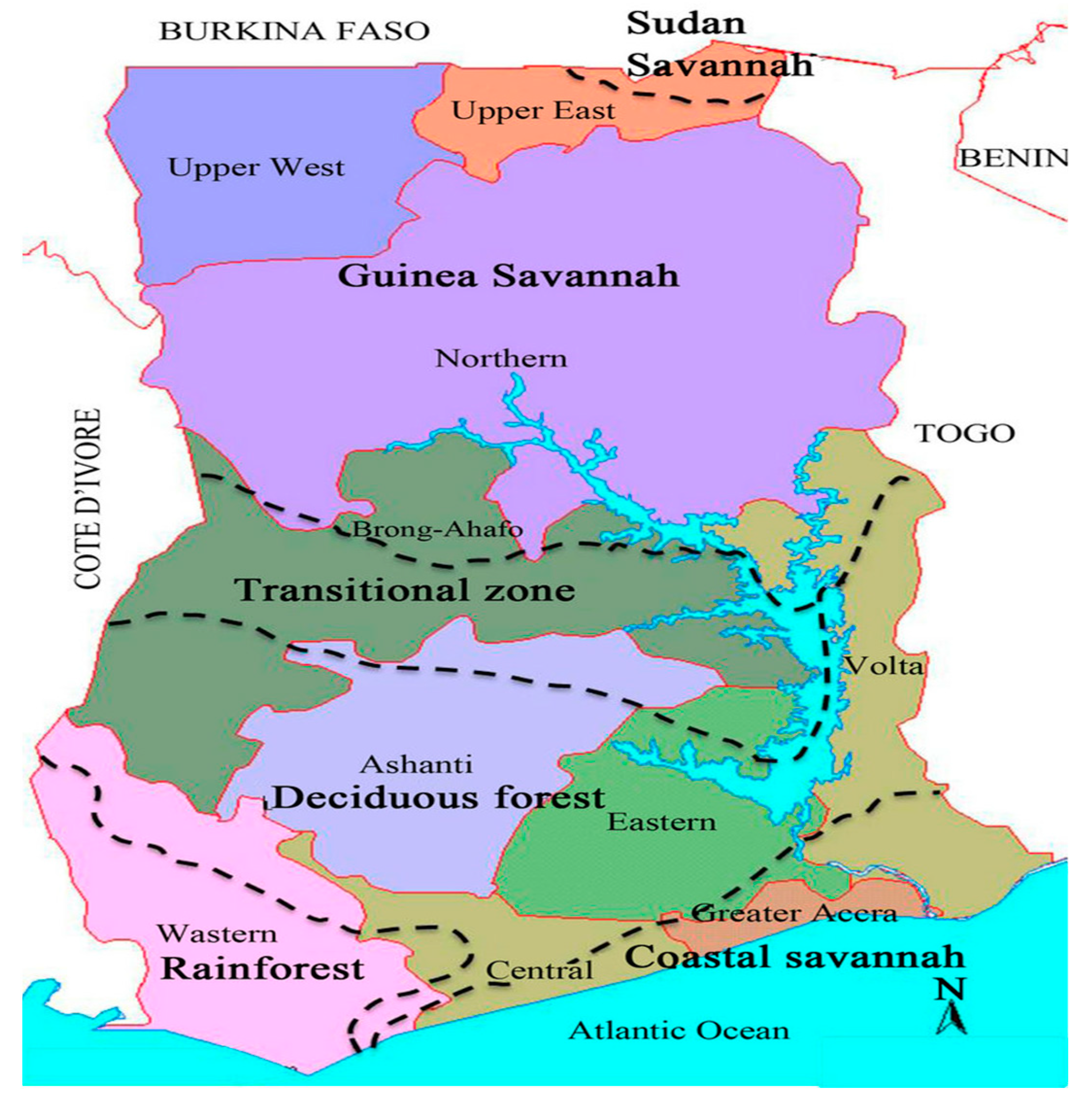
2.1. Climate Change and Variability in Ghana

The regional scenarios of seasonal precipitation and temperature changes in 32 regions globally analysed by (IPCC, 2014) show the current variations in climate and the range of variations in 30-year period predicted by GCM, focused in 2025, 2055, and 2085. This background information is critical in explaining the probable effects of climate variation on livestock and crop production.

The IPCC approximate that the past period saw temperatures increased by an average of 0.6 °C. The preceding 25 years, there was no observation of atmospheric temperatures from 1995–2006, 11 out of 12 was the warmest years [51]. Countries are beginning to experience consequences related to global warmings, such as the long-term drought within the Sahel zone in Africa and the expansion of the malaria transmission belt of tropical Africa [52]. Universally, the figure noted for weather-associated natural adversities is fast increasing. From the 1960s, accounts of natural risks have tripled. During 2007, fifteen (14) out of fourteen (15), “emergency appeals” for emergency public-spirited assistance were in the areas of storms, droughts and floods, five times more than in the prior year [53]. Ghana’s, climate variation is experiencing increasing unpredictable rainfall and temperatures in all regions [54].

Also, global warming is predicted to show variations in rainfall patterns, acidification, and moisture [55]. In this context, the global effect of climate variation on global life-assistance systems remains uncertain. Some parts experience extreme precipitation resulting in flooding; for example, the Mediterranean areas are experiencing a decline that could result in drought conditions [55]. By some reports [55], the anticipation of global average temperatures will rise between 1.4–5.8 °C by close of the century, as sea levels, increase as melting glaciers melt. Observations recently, however, indicate that many predictions concerning climate change are near the higher limit of the IPCC estimates. Sea levels, for example, have exceeded the IPCC estimates of up to 30 cm [56].

Based on a study by Reference [57], is establish that an estimated 35% of the entire land in Ghana is affected by increasing desertification. The unexpected variability of precipitation patterns is observed for years in Ghana as affirmed by Reference [58]. With the historical data, precipitation was mostly high in the 1960s, but fell to low levels by the end of 1970s and then rose again in 1980s. This fall in precipitation patterns is still prevalent currently, as Reference [59], with 20 years of data, observed this; temperatures are rising throughout Ghana and is precipitation decreasing and becoming gradually unpredictable. The effects of changing climate are anticipated to be severe in Ghana, even though there are rises and fall in both yearly temperatures and precipitation. Conceding to the World Bank’s projection, the temperature trend from 2010–2050 shows warming in almost the highest-temperature parts of Ghana, including the North and the Upper Regions.

Nevertheless, the region with the lowest temperature is the Brong Ahafo region. These are base on different climate scenarios [58]. For example, looking at the scenario, it was recognised that the temperatures of the three northern regions would increase by 2.1–2.4 °C by 2050. On the contrary, the predicted increase in Ashanti, West, East, Volta, and Central regions ranges from 1.7–2.0 °C and those of Brong Ahafo 1.3–1.6 °C.

We also reviewed the latest temperature and precipitation forecasts from the Intergovernmental Panel on Climate Change (IPCC) [60] to simulate the impact of climate change on agricultural production in Ghana. These projections are on Phase Five of the Coupled Model Inter-comparison Project (CMIP5), which brings together the results of 39 different global models. We used projections for West Africa until 2035. According to the first scenario, the most optimistic, the temperature should increase by 0.7 degrees and precipitation by 8%. These increases represent the expected minimum increase in temperature and the maximum expected increase in precipitation. The second scenario concerns the median increase in temperature (0.9 degrees) and precipitation (1%). The third scenario, the least optimistic, concerns the maximum expected increase in temperature (1.5 degrees) and the maximum decrease in precipitation (4%). A meta-analysis of crop yield response to climate change, using local average temperature as an indicator of change, concluded that global warming at 2 °C could lead to an increase in wheat, rice, and maize yields, with yields subsequently decreasing with increased warming. The AR4 also showed that crop-level adaptations had a markedly positive effect on all crops, regions, and warming levels [61].

According to Reference [62],

Table 1. The projections of precipitation in Ghana.

Location	Climate Type	Forecast Changes
Accra	Coastal Savanna Zone	From 52% decreases to 44% increases in wet season rainfall by the year 2080.
Kumasi	Deciduous Forest Zone	From 48% decreases to 45% increases in wet season rainfall by the year 2080. Based on their A2 scenario, which generally shows the largest greenhouse gas (GHG) impact, predicts the weakest increase in wet season rainfall, 1.13%.
Tarkwa	Rain Forest Zone	From 45% decreases to 31% increases in wet season rainfall.
Techiman	Forest-Savanna Transition Zone	From 46% decreases to 36% increases in wet season rainfall. The A2 scenario, which generally shows the largest GHG impact, predicts the largest decrease in wet season rainfall, −2.94%.
Tamale	Guinea Savanna Zone	From 36% decreases to 32% increases in wet season rainfall consistent trend toward decreased rainfall.
Walembelle	Northern Guinea Savanna Zone	From 25% decreases to 24% increases in wet season rainfall
Bawku	Sudan Savanna Zone	Range from 28% decreases to 30% increases in wet season rainfall.

Source: Extracted from [8,43].

and

Table 2. Temperature projections in various climate stations in Ghana.

Location	Climate Type	Temperature Projections
		Wet Season	Dry Season
Accra	Coastal Savanna Zone	1.68 ± 0.38 °C by 2050 2.54 ± 0.75 °C by 2080	1.74 ± 0.60 °C by 2050 2.71 ± 0.91 °C by 2080
Kumasi	Deciduous Forest Zone	1.71 ± 0.39 °C by 2050 2.60 ± 0.77 °C by 2080	1.81 ± 0.68 °C by 2050 2.83 ± 1.04 °C by 2080.
Tarkwa	Rain Forest Zone	1.69 ± 0.37 °C by 2050 2.56 ± 0.75 °C by 2080	1.76 ± 0.67 °C by 2050 2.76 ± 1.01 °C by 2080.
Techiman	Forest-Savanna Transition Zone	1.77 ± 0.43 °C by 2050 2.71 ± 0.85 °C by 2080	1.95 ± 0.79 °C by 2050 3.05 ± 1.20 °C by 2080.
Tamale	Guinea Savanna Zone	1.84 ± 0.46 °C by 2050 2.83 ± 0.91 °C by 2080	2.05 ± 0.75 °C by 2050 3.18 ± 1.18 °C by 2080.
Walembelle	Northern Guinea Savanna Zone	1.92 ± 0.52 °C by 2050 2.96 ± 0.98 °C by 2080	2.10 ± 0.71 °C by 2050 3.27 ± 1.11 °C by 2080.
Bawku	Sudan Savanna Zone	1.92 ± 0.53 °C by 2050 2.97 ± 0.98 °C by 2080	2.11 ± 0.68 °C by 2050 3.25 ± 1.08 °C by 2080

Source: Extracted from [8,43].

show some of the climate changes in Ghana and the corresponding time periods.

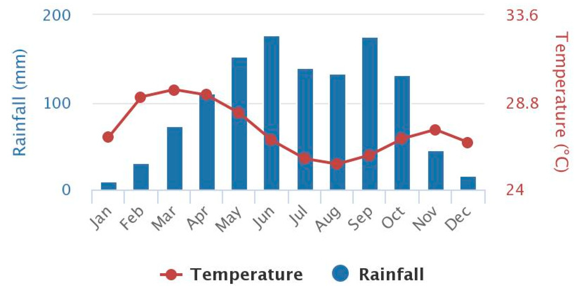
2.2. Seasonal Changes of Precipitation and Temperature

The climate of Ghana is tropical, with a dry season in winter and a rainy season during the summer due to an African monsoon. The duration of the rains varies according to the ecological zones. As shown in Figure 1, the rainy season is usually from May to September to the north, from April to October in the centre, and from April to November to the south. However, on the east coast, the rainy season is shorter than the rains from April to June, with no rainfall in July and August, and it picks up slightly in September and October. The south is the coolest part of Ghana, where it has more than 1500 mm (per year), and even more the small west coast, where it reaches 2000 mm (80 inches) per year. The north is the driest in Ghana, where rainfall is about 1000 mm (40 inches) per year and the east coast, including the city of Accra, where it falls below 800 mm (31.5 in).

2.3. The trend of Climate Change in Ghana

Ghana is located in West Africa, bordered to the north by Burkina Faso, east to Togo, west to Ivory Coast, and south to the Gulf of Guinea. It is located between 4.50 degrees north and 11.50 degrees north and longitude 3.50° west and 1.30° east. The country has an area of 239,460 Km² and a surface area of 8520 Km² as seen in Figure 2. The country has a population of around 24 million since 2010, with an annual growth rate of about 2.5% [63]. Young people dominate this population. The main exports are cocoa, gold, wood, diamonds, bauxite, manganese, and hydroelectricity. Until recently, the country also began to export crude oil. In 1991/92, the poverty level in Ghana reached 51.7 per cent, and this figure has steadily declined in recent years to 39.5 per cent in 1998/99, 28.5 per cent in 2005/06, and 24.2 per cent in 2012/2013. The country enjoys a high temperature while the average annual temperature is between 24 °C and 30 °C. Despite the average annual temperature, temperatures may be 18 °C and 40 °C in the southern and northern parts of Ghana. Rainfall in Ghana is generally declining from south to north. A more prosperous region in Ghana is the far southwest, with an annual rainfall of about 2000 mm. However, the annual rainfall in northern Ghana is less than 1100 mm. The country has two major systems of rain: the double-twin system and the single maximum regime. For the maximum binary system, the maximum periods are from April to July and from September to November in southern Ghana. While the only maximum system is from May to October in northern Ghana, the prolonged drought lasts from November to May. Over the years, temperatures have risen in all ecological regions of Ghana, while rainfall levels have generally declined and standards have steadily increased [9].

Despite dramatic improvements in technology and crop yields, food production continues to depend heavily on the climate because solar radiation, temperature and rainfall are the critical factors of increase in crop production. The climate is affected by the diseases of plant and the spread of pests, including the supply and demand for irrigation water. For instance, in recent decades, the ongoing drought in the Sahel has caused a continued deterioration in food production [64] in Ghana. The effect of the changing climate on crops was in 1990, where the crop has suffered or decreased. Also, due to drought, climate indicators such as rainfall and average mean temperature are associated with crop change [57].

Table 3. Climatic variations experienced in Ghana.

Time Period	Climatic Variations
January–July 1976	Scorching weather conditions
1983–1984	Drought: A yearlong of bushfires
October–December 1989	Scorching weather conditions
1991	Lots of rains throughout the year
1995	About 40 days of intensive rains
2004	Noticeable are frigid winds during March–April (Easter) and November–January was very cold weather
2005	Cold periods resulting in animal deaths
August 2006	One week of intensive rains, and
2007	Lots of rains in August and September.

Source: Extracted from [62].

below presented climate change variations experienced.

2.4. The Generalized Extreme Value Distribution (GEVD)

The GEVD is part of the family of continuous distribution functions that allows a continuous range of shapes and consists of classes of distribution functions such as Gumbel, Fréchet, and Weibull. Considering the Fisher-Tippett Gnedenko theorem, the GEVD is a limit-form distribution function, which maximises the maxima of the sequence of random variable considered as independent and identical distributed (i.i.d). It, therefore, models the maximum of a finite sequence of random variables. The combined model of maxima is by Equation (1):

$$\begin{array}{l}{G}_{\gamma ,\mu ,\sigma }=\exp \left\{-\left(1+\gamma {\left(\frac{x-\mu }{\sigma }\right)}^{-\frac{1}{\gamma }}\right)\right\}\mathrm{with},\gamma \ne 0,\sigma >0\mathrm{and}\gamma \left(\frac{x-\mu }{\sigma }\right)>0\\ \sigma >0\end{array}$$

(1)

The derivative of Equation (1), give a probability density function in Equation (2) as:

$$g_{\gamma ,\mu ,\sigma }=\frac{1}{\sigma }{\left(1+\gamma \left(\frac{x-\mu }{\sigma }\right)\right)}^{-1-\frac{1}{\gamma }}\exp \left\{-{\left(1+\gamma \left(\frac{x-\mu }{\sigma }\right)\right)}^{-\frac{1}{\gamma }}\right\},\gamma \ne 0$$

(2)

where $\mu$ and $\sigma$ are the location and scale parameters, respectively [20].

The GEVD shape parameter $\gamma$ also termed as the extreme value index. The decay rate of GEVD seen as ${\gamma }^{-1}$. If $\gamma >0$ for a class of distributions, G fits distributions as; the heavy-tailed Fréchet distribution, Cauchy, Student’s t, Pareto class, and mixture other distributions. G fit into the short-tailed Weibel distribution, uniform, and beta distribution if $\gamma <0$. G fits the right-tailed Gumbel distributions (normal, exponential, gamma, and lognormal) if $\gamma =0$ [65,66,67].

2.5. Maximum Likelihood Estimation for GEVD

The assumption that X₁, …, X_m follows an (i.i.d) and also from generalised extreme value distribution with parameter when $\gamma \ne 0$ the log-likelihood function given as:

$$\mathrm{Provided}\mathrm{that}1+\gamma \left(\frac{x_{(i)}-\mu }{\sigma }\right)>0\mathrm{for}i=1,2,\dots ,m$$

(3)

$$l\left(\mu ,\sigma ,\gamma \right)=-m\ln \sigma -\left(1+1/\gamma \right){\displaystyle \sum _{i=1}^m\ln \left[1+\gamma \left(\frac{x_{(i)}-\mu }{\sigma }\right)\right]}-{{\displaystyle \sum _{i=1}^m\left[1+\gamma \left(\frac{x_{(i)}-\mu }{\sigma }\right)\right]}}^{-1/\gamma }$$

(4)

Parameters combination that deviates from the above conditions (Equation (3)), i.e., in a configuration where at least one of the observed data exceeds the endpoint of the distribution (Equation (4)), the likelihood is zero, and the log-likelihood is equal to −∞. This case $\gamma =0$ requires separate treatment with GEVD’s Gumbel restriction leading to logarithmic log-likelihood as in Equation (5);

$$l\left(\mu ,\sigma \right)=-m\ln \sigma -{\displaystyle \sum _{i=1}^m\left(\frac{x_{(i)}-\mu }{\sigma }\right)}-{\displaystyle \sum _{i=1}^m\exp \left\{-\left(\frac{x_{(i)}-\mu }{\sigma }\right)\right\}}$$

(5)

Equations (2) and (3) are differentiated and maximised concerning the parameter vector $(\mu ,\sigma ,\gamma )$, Solving for $(\mu ,\sigma ,\gamma )$, results to the maximum likelihood estimates for the whole GEVD model [20,28,68,69]. Maximum likelihood estimation offers the advantage of estimation of the three parameters together and applicable to the series of maxima per block [70].

Model Checking for GEVD

The model fit of GEVD measure after estimating the parameters by utilising residual plots function as defined by Equation (6),

$$res=\{\begin{array}{ll}{\left(1+\frac{\gamma }{\sigma }\left(x-\mu \right)\right)}^{-1/\gamma }& if\gamma =0\\ \exp \left[-\exp \left(-\frac{x-\mu }{\sigma }\right)\right]& if\gamma \ne 0\end{array}$$

(6)

Ascertain by Reference [20] conversion of data to unit exponential distributed residuals is on the null assumption that GEVD fits the data.

2.6. Return Period or Level Estimates

The frequency of extreme quantiles incidence estimated with a fixed value of return level. The return level is the mean number of events taking place within a unit period, e.g., one year [71]. Return levels are essential for prediction purposes and estimated from stationary models. The expected return time is the number of time (years) one is expected to wait on average before the observation of another extreme event of at least the same intensity. If a threshold exceedance of a given probability of an observed extreme incidence in any given time (year) is p, then the mean return period T is such that $T=1/p$.

2.7. Test for Stationarity and Seasonality

The stationarity of the data conducted by the augmented Dickey-Fuller (ADF) stationarity test on the assumption that there is no trend [72]. The quality of convergence of the weather extremes is access using the Kolmogorov–Smirnov (K-S) and Anderson–Darling goodness-of-fit tests. The K-S test, relying on the empirical study of the cumulative distribution function, is used to determine whether the sample is from the hypothesised continuous distribution. The K-S approach is less sensitive for normal distribution [72]. The Anderson-Darling test, an enhancement of the K-S test, compares the fit to the expected cumulative distribution function of the observed cumulative distribution function. This test gives more substantial weight to the tail of the distribution than the K-S test [72].

The assumption is that the data is from a population which is independent identically distribution (i.i.d). The alternative hypothesis is a two-tail test on the assumption that the data follow a monotonic trend. Thus, the following test statistics by Mann-Kendall determine by Equation (7):

$$S={\displaystyle \sum _k^{n-1}{\displaystyle \sum _{j=k+1}^n\mathrm{sgn}\left(x_j-x_k\right)}}$$

(7)

with sgn the signum function.

3. Methodology

This paper analyses past Composite Indexes in Agriculture ranges from 1961–2016: crops production, cocoa production, livestock production, cereal production, and food production in Ghana. The data also consider records of maximum rainfall, maximum temperature, and minimum temperature value as weather indicators from January 1965 till July 2016. We sourced the data from the Ghana Meteorological Agency for climate data, and agriculture production indexes from the Food and Agriculture Organization also in Ghana. Rainfall and temperature are assumed to be the primary determinants of weather in Ghana as seen in Figure 1. The first task was to check for stationarity of the weather variables using Augmented Dickey-Fuller (ADF) unit root test and then the Mann-Kendall Trend Test of seasonality. It was necessary to apply methods that explicitly allow for testing non-stationarity in the distribution parameters of climate variables [20].

Next step was to model from the dataset of the weather indicators employing the Block Maximum Method for the weather extremes under Generalized Extreme Value Distribution (GEVD). There were two approaches to the modelling of Block minima data for the minimum temperature. Either the GEVD for minima fitted to this data or the data negated and the GEVD for maxima fitted [20]. The latter approach was adopted since the Extremes Toolkit does not include a routine to estimate the GEVD for minima directly. The block maxima method is a parametric approach to Extreme Value Theory. It entails fitting the GEVD to a specific group of maximum values chosen in a given sample of data. It focuses on the statistical behaviour of the largest or smallest value in a sequence of independent random variables. Assume that the sequence is grouped into blocks of size N (with a reasonably large number) and that only the maximum score $M_i\left(i=1,2,3,\dots ,n\right)$ of each block extracted. Each $M_i\left(i=1,2,3,\dots ,n\right)$ of the weather indicators is then used to estimate the relationship between the composite indexes of agriculture production.

The mean return period defines the amount of time (e.g., years) that is expected to pass on average before a new extreme with the same or increased intensity. Given the likelihood that events past a certain threshold will follow an extreme of a particular security at any given time (year) is defined as p, then the mean return period T can be calculated as $T=1/p$.

Food production index includes food crops that are considered edible, and that contain nutrients with the exclusion of coffee and tea because they have no nutritive value although edible (FAO). Figure 3 shows the primary crop food calendar.

Finally, we investigated the relationship between extreme weather events and agriculture production using SEM software to evaluate the potential impacts of weather extremes on Agriculture production. We used SEM regression for the paths equation modelling analysis with the partial least squares (SEM) estimation technique [73]. SEM is a modelling approach with a flexible procedure, which can handle data with missing values, strongly correlated variables, and small samples. SEM-regression works with both continuous and discrete observed variables as indicators. The SEM estimates loading and path parameters between variables and maximises the variance explained for the outcome variables [73].

4. Results and Discussion

4.1. Stationarity Test for the Weather Indicators

The ADF test is captured in

Table 4. Stationarity and Seasonality test.

Augmented Dickey-Fuller Stationarity Test
Test Variable		Test’s Critical Values			Test Statistics	p-Value
		1%	5%	10%
Annual maxi. Rainfall		−3.958	−3.410	−3.127	−16.350	0.0000
Annual maxi. Temperature		−10.007	−3.431	−2.862	−2.567	0.0000
Annual mini. Temperature		−12.482	−3.431	−2.862	−2.567	0.0000
Seasonal Mann-Kendall Trend Test
Series	Statistics		p-value		tau	Slope 95% CI
	z (trend)	z (Het)	p (trend)	p (Het)
Maxi. Rainfall	0.434	22.376	0.664	0.0216	0.0019	0.0044 [−0.0194,0.0308]
Maxi. Temperature	21.842	4.779	<0.001	0.9410	0.1320	0.0318 [0.0286,0.0346]
Mini. Temperature	25.123	23.894	<0.001	0.1320	0.1520	0.0231 [0.0212,0.0250]

95% confidence interval in parenthesis.

indicating the significance of the p-value statistics. The premise of non-stationary at 1%, 5%, and 10% rejected, and therefore we conclude the stationarity of the weather indicators.

It is reported by scholars that, Mann-Kendall Trend Test of stationarity is reliable and efficient. In line with this, analysing environmental data demands the exposure of movements of events on separate points [74]. Based on this, the test outcome illustrates high or low trends in weather conditions of a particular jurisdiction.

In Table 4, the estimated annual trend is 0.0044 mm/year, a yearly increase in the maximum annual rainfall. The p-value based on the Kendall seasonal trend test is p = 0.6640, which shows no importance. The 95% confidence interval on both sides for the trend (−0.014,0.0307), the chi-square test for heterogeneity (Het) gave a p-value of 0.0216. Therefore, there is a difference in the level of a trend in the different seasons of the maximum annual rainfall. As shown in Table 4, the estimated annual trend is 0.0318 degrees Celsius (°C)/year, which is a yearly increase in the yearly maximum temperature. The p-value corresponds to the Kendall seasonal test for the p < 0.001 trends, indicating that it is statistically significant. The 5% level of significance on both sides for the trend is (0.0286, 0.0346). The chi-square heterogeneity test (Het) provides a p-value of 0.9410, so there is no evidence for different sets of stresses at different times of the maximum annual temperature. The estimated annual trend is 0.0231 degrees Celsius (°C)/year, a yearly increase in the maximum annual temperature. The p-value of the Kendall seasonal trend test, p < 0.001, indicating that it is statistically significant. The 5% level of significance on both sides for the trend is (0.0212,0.0250). The chi-square test for heterogeneity (Het) gives a p-value of 0.1318, i.e., no indication of the different trend in different seasons of the minimum annual temperature.

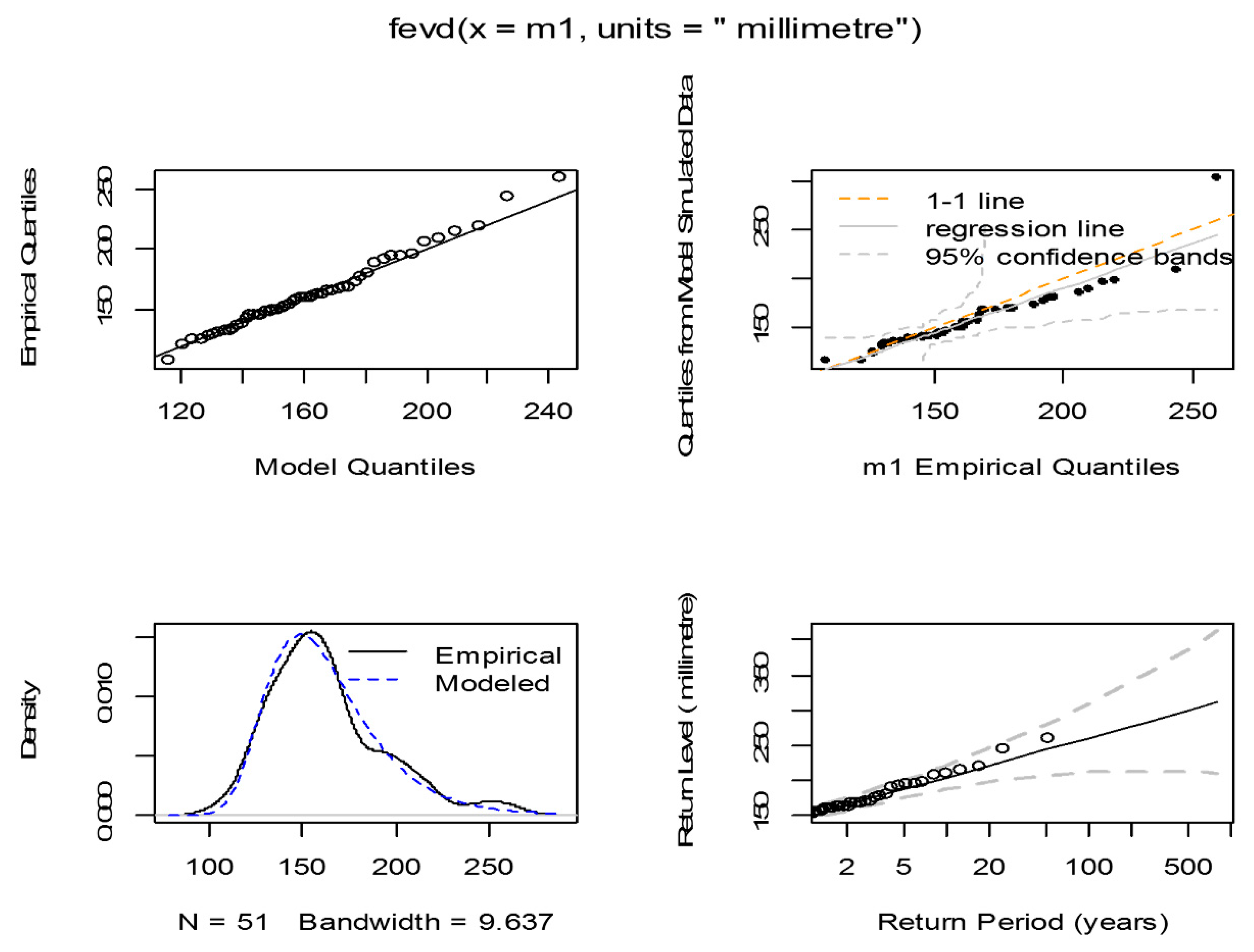
4.2. GEVD Model for Extreme Maximum Rainfall

In

Table 5. Generalised extreme value estimates of maximum rainfall.

GEV	Maximum Rainfall
	Location	Scale	Shape
Estimates	$\mu$ = 149.03	$\sigma$ = 23.98	$\gamma$ = 0.0024
Std error	3.758	2.718	0.1002
95% CI (normal app)	(141.67,156.39)	(18.65,29.31)	(−0.193,0.198)
Estimated Return Levels	95% Lower	Estimate	95% Upper
5-year return level	173.14	185.06	196.98
10-year return level	186.59	203.13	219.68
20-year return level	196.99	220.50	244.03
50-year return level	206.49	243.04	279.57
100-year return level	210.72	259.95	309.05

, the estimated return periods of maximum rainfall likely to occur over the next 5, 10, 20, 50 or even 100 years fitted by GEVD. The estimated results are $\left(\mu ,\sigma ,\gamma \right)$ (149.03,23.98,0.0024), with standard errors (3.758, 2.718, 0.1002). The approximate 95% confidence intervals for the parameters are thus (141.67, 156.39) for $\mu$, (18.65, 29.31) for $\sigma$, and (−0.193,0.198) for $\gamma$.

The validity and reliability of the extrapolation of GEVD fit is assessed base on the observed data. Four graphical analyses assist with model checking [20,75]. Figure 4 shows diagnostic plots assessing the accuracy of the GEVD model fitted. Neither the quantile plot nor the density plot has any reason to doubt the validity of the fitted model: each drawn set of points is almost linear. The return level plots asymptotically converge to a determinate value due to the positive estimates, with the curve approaches a straight line. The sample variable under consideration provides an adequate representation graphically of the empirical estimates. Finally, the corresponding density estimate appears to be consistent with the density curve. As a result, all four diagnostic diagrams support the GEVD model as in Figure 4 (Top-left: empirical plot; Top-right: empirical quartile plot; Bottom-left: density plot; Bottom-right: return level plot).

The determination of the limiting distribution by maximising the GEV negative log-likelihood for annual maximum rainfall leads to the following function in Equation (8):

$$G\left(z\right)=\exp \left\{-{\left[1+0.00243\left(\frac{z-23.98}{149.03}\right)\right]}^{\raisebox{1ex}{$-1$}\!\left/ \!\raisebox{-1ex}{$0.00243$}\right.}\right\}$$

(8)

Equation (8) gave estimates of return levels for 5, 10, 20, 50, and 100-years and their 5% significant level as shown in Table 3. Thus, based on the data from 1965 to 2016, once in 50 years we should expect to see an extreme annual maximum rainfall hit between 206.5 and 279.6 mm. The upper bound of the model prediction for the 50-years Return level of 279.6, but 510 mm extreme rainfall recorded in 1968. Of course, this is undoubtedly extreme beyond regular extreme events, which is not expected based on the model’s predictions. Results from Table 2, indicates that extreme maximum rainfall is steadily increasing significantly over the 100 years.

4.3. GEVD Model for Extreme Maximum Temperature

As shown in

Table 6. GEVD estimates of maximum temperature.

GEVD	Maximum Temperature
	Location	Scale	Shape
Estimates	$\mu$ = 42.08	$\sigma$ = 0.826	$\gamma$ = −0.292
Std error	0.128	0.0912	0.0942
95% CI (normal app)	(41.664,42.202)	(0.686,1.098)	(0.046,0.359)
Estimated Return Levels	95% lower	Estimate	95% upper
5-year return level	42.82	43.08	43.35
10-year return level	43.16	43.44	43.72
20-year return level	43.39	43.72	44.04
50-year return level	43.59	44.00	44.41
100-year return level	43.67	44.17	44.67

, the estimated return level of maximum temperature likely to occur over the next 5, 10, 20, 50, or even 100 years by fitting these data to the GEVD. The maximum rainfall data yield estimates for $\left(\mu ,\sigma ,\gamma \right)$ of (41.933,0.892, 0.203), with standard errors (0.137,0.105,0.079). The approximate 95% confidence intervals for the parameters are thus (41.66,42.20) for $\mu$, (0.686,1.098) for $\sigma$, and (0.0463,0.359) for $\gamma$.

Analytic plots used in estimating the accuracy of the GEVD model fitted to the annual maximum temperature data shown in Figure 5 (Top-left: empirical plot; Top-right: empirical quartile plot; Bottom-left: density plot; Bottom-right: return level plot). All four diagnostic schemes provide support for fitting the GEVD to the maximum annual temperature.

The determination of the limiting distribution by maximising the GEV negative log-likelihood for annual maximum temperature leads to the following function, Equation (2): $\left(\mu ,\sigma ,\gamma \right)$ of (42.081, 0.826, −0.292)

$$G\left(z\right)=\exp \left\{-{\left[1+0.826\left(\frac{z-0.892}{42.08}\right)\right]}^{\raisebox{1ex}{$-1$}\!\left/ \!\raisebox{-1ex}{$-0292$}\right.}\right\}$$

(9)

From Equation (9), estimates of return periods for 5, 10, 20, 50, and 100-years and their confidence intervals at 95% as shown in Table 6. Thus, based on the data from 1965 to 2016, once in 100 years we should expect to see an extreme annual maximum temperature hit between 43.6 °C and 44.4 °C maximum temperature. The upper bound of the model prediction for the 100-years return is 44.4 °C, but 65 °C extreme annual temperature recorded in 1989. Of course, this is also undoubtedly extreme beyond regular extreme events, which is not expected based on the model’s predictions. It is revealed by Table 6, that extreme maximum temperature consistently increasing marginally over the 100 years.

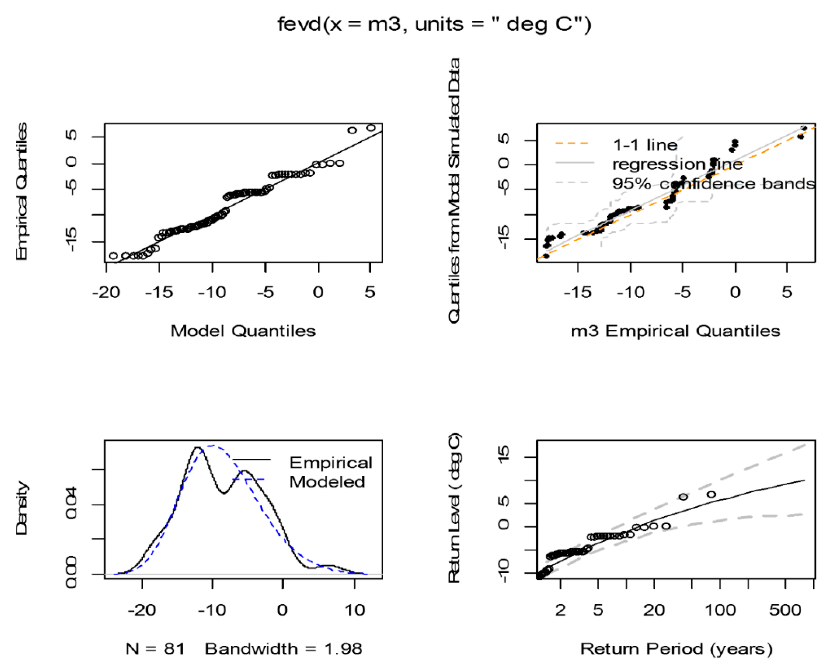
4.4. GEVD Model for Extreme Minimum Temperature

In

Table 7. GEV estimates of Minimum Temperature.

GEV	Minimum Temperature
	Location	Scale	Shape
Estimates	$\mu$ = 6.408	$\sigma$ = 5.261	$\gamma$ = −0.632
Std error	0.817	0.758	0.148
95% CI(normal app)	(4.806,8.011)	(3.774,6.747)	(−0.922,−0.342)
Estimated Return Levels	95% lower	Estimate	95% upper
5-year return level	10.355	11.506	12.657
10-year return level	11.882	12.723	13.564
20-year return level	12.761	13.456	14.151
50-year return level	13.233	14.022	14.812
100-year return level	13.333	14.274	15.216

below, the estimated return periods of minimum rainfall likely to occur over the next 5, 10, 20, 50 or even 100 years fitted to the GEVD. The maximum rainfall variable yields estimates for $\left(\mu ,\sigma ,\gamma \right)$ of $\left(6.408,5.261,-0.632\right)$, with standard errors (0.817, 0.758, 0.148) respectively. Approximate 95% confidence intervals for the parameters are thus (4.806, 8.011) for $\mu$, (3.774, 6.747) for $\sigma$, and (−0.922, −0.342) for $\gamma$.

Equation (10) is the determination of the limiting distribution by maximising the GEV negative log-likelihood for annual minimum temperature leads to the following function:

$$G\left(z\right)=\exp \left\{-{\left[1-0.632\left(\frac{z-5.261}{6.408}\right)\right]}^{\raisebox{1ex}{$-1$}\!\left/ \!\raisebox{-1ex}{$(-0.632)$}\right.}\right\}$$

(10)

Supposing the relative stability of the GEVD process producing estimates for annual minimum temperature in degree Celsius (°C), the model estimates that the 5-year return level is 11.5 °C with 95% confidence interval (10.4, 12.7). For ten years it is a 12.7 °C extreme minimum temperature with 95% confidence interval (11.9, 13.6), and for 50 years it is 14.0 °C extreme minimum temperature with 95% confidence interval (13.2, 14.8). Thus, based on the data from 1968 to 2016, once in 100 years we should expect to see an extreme annual minimum temperature hit between 13.3 °C and 15.2 °C. For the period under annual extreme minimum temperature, there was no extreme beyond normal extreme events. In Table 7, the extreme minimum temperature is consistently increasing over the 100 years’ duration. In Figure 6 (Top-left: empirical plot; Top-right: empirical quartile plot; Bottom-left: density plot; Bottom-right: return level plot), all four diagnostic schemes provide support for fitting the GEVD to the minimum annual temperature.

4.5. Return Level

Given 50-year return level for each of the indicators of extreme weather (for the year 2076), the return levels of extreme maximum rainfall in Ghana is higher than 150 mm reaching a warning line of extremely torrential rain, as defined by the Meteorological Service of Ghana. Similarly, the 50 years return level for maximum temperature exceeds 40 °C reaching a warning line of unusual temperature as defined by the Meteorological Service of Ghana. Also, the 50 years return level for extreme minimum temperature is lower than 20 °C reaching a warning line of frigid cold, as defined by the Meteorological Service of Ghana.

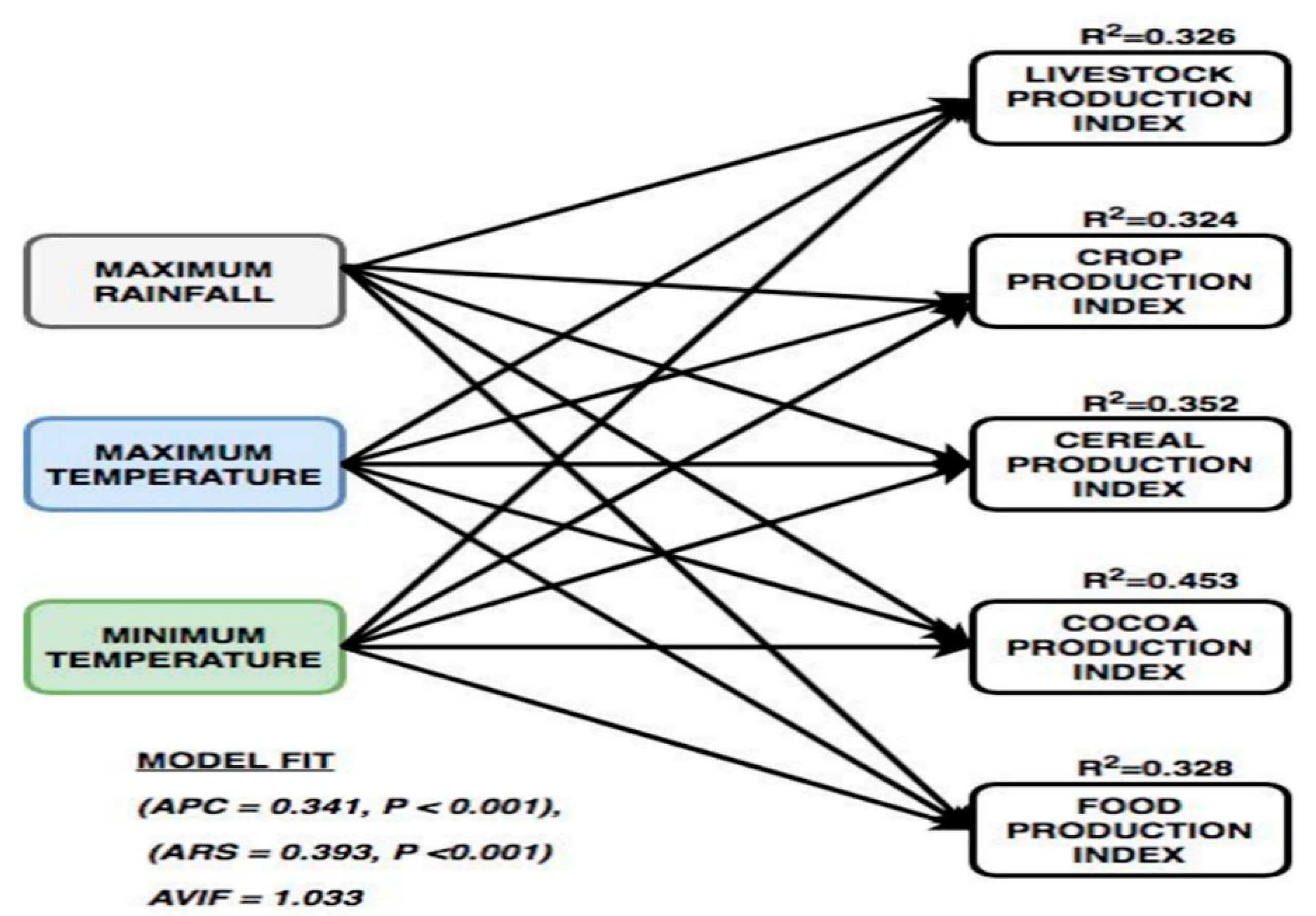
4.6. Structural Equation Modeling (SEM)-Regression Analysis

The term “structural equation modelling” (SEM) conveys two significant phases of the process: (a) causal effects under the research epitomised by a lot of structural equations (i.e., regression), and (b) these structural relationships can be presented to enable more specific concepts of theory studying. The assumed model (Figure 7) can then be statistically tested in a simultaneous analysis of the entire variables system to determine its compatibility with the data. If the suitability is appropriate, the model argues for the acceptance of assumed interactions between the variables; if inappropriate, the likelihood of such relationships fails to accept [76]. We chose PLS-SEM in present work for the following reasons: It is suitable for studies of theory construction [77,78]. It is appropriate to assess the sophisticated models of the cause-effect interaction [79,80]. The PLS-SEM assume a non-boundary approach, with fewer restrictions regarding sample size and data distribution [77].

SEM-regression estimation procedure was used to examine the hypothesised relationships as shown in Figure 4 between weather indicators and agriculture production. The results of SEM analysis showed a significant correlation between extreme weather and Agriculture production.

4.6.1. The relationship between Maximum Rainfall and Composite Agriculture Indexes

The analysis as showed in

Table 8. Standardised Regression Weights and significance of correlations.

Predictor	Outcome	Path Coefficient	p-Values
Maximum Rainfall	Livestock Production Index	−0.184	0.144
	Crop production index	−0.189	0.133
	Cereal Production index	−0.266 *	0.031
	Cocoa production	−0.461 ***	<0.001
	Food Production Index	−0.190	0.131
Maximum Temperature	Livestock Production Index	0.305 *	0.015
	Crop production index	0.263 *	0.037
	Cereal Production index	0.276 *	0.025
	Cocoa production	0.424 *	0.023
	Food Production Index	0.268 *	0.033
Minimum Temperature	Livestock Production Index	0.457 ***	<0.001
	Crop production index	0.482 ***	<0.001
	Cereal Production index	0.415 ***	<0.001
	Cocoa production	−0.211 *	0.038
	Food Production Index	0.484 ***	<0.001

Significance of coefficient: *** p < 0.001 and * p < 0.050.

is that, Livestock production index ($\beta$ = −0.1840, p = 0.144), crop production ($\beta$ = −0.189, p < 0.133), Cereal production ($\beta$ = −0.266, p < 0.031), Cocoa ($\beta$ = −0.461, p < 0.001), and food production index ($\beta$ = −0.190, p < 0.131). Each is influenced by the effect of extreme maximum rainfall negatively on all composite agriculture indexes with no significant effect on crop production, food production, and livestock indexes. There has been a significant effect on cereal production and cocoa production indexes.

The results as shown in Table 8, shows each index is influenced by the effect of extreme maximum rainfall negatively, with no significant impact on crop production, food production, and livestock indexes. There has been a considerable effect on cereal production and cocoa production indexes. Maximum extreme rainfall hurts the performance of cereals.

Consequently, a unit increase in maximum extreme rainfall leads to a decrease in cereal production by 0.266 units. Maximum extreme rain leads to filtration of essential nutrients necessary for grain growth. Under such condition, any nutrient whether organic or inorganic leached beyond the reach of the roots, will result in reduced yields.

For cereals to bear maximum yields, rainfall, especially during tasseling for maize, is needed in moderation, inter-sparse with sunlight for maximum yields. Torrential rains do not favour most crops production and most especially cereals. Several studies have shown the importance of rainfall variability in crop production in various spatial scales [33,38].

Excessive rain has an adverse impact on agriculture. These effects run via different mechanisms. Heavy rains and floods have resulted in crop damage and the creation of poor conditions for harvesting, storage and transport of agricultural products. It is not astonishing that maximum rainfall has a negative association with all the variables under consideration, but only cereal and cocoa production indexes are statistically significant. Rainfall affects more variations in cocoa yields from year to year than with any other climatic factor. Trees are prone to a soil water shortage. The rain should be abundant and well distributed throughout the year. The annual precipitation between 1500 mm to 2000 mm is generally preferred. Droughts with rainfall below 100 mm per month should not exceed three months. The flooding of farmland leads to the leaching of nutrients needed for the growth of cocoa trees. If the phenomenon occurs over a period, this often leads to the death of cocoa trees or poor yields are observed [81]. It affects the flowering of cocoa trees and leads to flower aborting in some instances.

4.6.2. The Relationship between Maximum Temperature and Composite Agriculture Indexes

As shown in Table 8, Livestock production index ($\beta$ = 0.305, p = 0.015), crop production ($\beta$ = −0.263, p = 0.037), Cereal production ($\beta$ = 0.276, p = 0.025), Cocoa ($\beta$ = 0.424, p = 0.023), and food production index ($\beta$ = 0.268, p < 0.033). Each is influenced significantly by the effect of extreme maximum temperature positively on all agriculture production indexes.

As shown in Table 8, each outcome is influenced significantly by the effect of extreme maximum temperature positively on all agriculture production indexes. The result indicates that a unit change in the maximum temperature will result in about 0.305 change in livestock production index. The nature of Ghana’s livestock production immune it from the effects of extreme temperature conditions. Most animals are subject to a free or semi-intensive management system where animals are about to move freely.

Also, most cattle raised in Ghana are more adaptable to the state of the coast. As a result, maximum temperatures in Ghana does not affect them negatively since most of the animal rearing areas are almost in the coastal savannah region where the temperatures are not as high as the actual Sahel regions.

Breeding animals are sensitive to climate change and are severely affected by heat stress with an adverse effect on reproductive function [44,82]. According to Reference [83], high temperature and radiant heat load affect the reproductive rhythm through the hypothalamohypophyseal-ovarian axis. The primary factor in regulating ovarian activity is GnRH of thalamus and gonadotropin, i.e., FSH and LH of the anterior pituitary wall.

Research by [84,85] showed that the LH pulse amplitude and frequency of heat stressed cattle decreased. However, this is not the case in Ghana as shown in the results. Extreme temperatures that result in detrimental conditions not recorded in Ghana. High extreme temperatures hurt the crop production index, cereals production index, cocoa production, and food production index.

The maize pollen viability declines at temperatures above 35 °C [86,87,88]. Temperature increases in the 21st century may lead to yield losses of between 2.5% and 10% in some agronomic species [46]. Other assessments of crop yield due to temperature have produced different outcomes. Studies conducted by [89,90] showed estimates of yield between 3.8% and 5% decreases According to [90], crop growth for maize, soybeans and cotton will increase gradually with temperatures ranging from 29 °C to 32 °C and then sharply decrease as temperatures rise above this limit. It is however not surprising that maximum temperature in Ghana does not have adverse effects on yields. Maximum temperatures in Ghana is from 29 °C to 32 °C recorded in a dry season where no cultivation is taking place.

The period for production is the rainy season where temperatures hardly get close to 29 °C to 32 °C. Cocoa especially requires much heat, but direct sunshine damages it. As a result, some level of protection is necessary, especially when trees are young. Cocoa trees respond well to moderately high temperatures with a maximum yearly mean of 30 °C to 32 °C [91]. It is however not surprising that maximum temperature associate positively with cocoa production in Ghana where the maximum temperature falls within the acceptable range for cocoa.

4.6.3. The Relationship between Minimum Temperature and Composite Agriculture Indexes

As shown in Table 8, livestock ($\beta$ = 0.457, p < 0.001), crop ($\beta$ = 0.482, p < 0.001), Cereal ($\beta$ = 0.415, p < 0.001), Cocoa ($\beta$ = −0.211, p = 0.038), and food ($\beta$ = 0.439, p < 0.001). Each is influenced significantly by the effect of extreme minimum temperature adversely on cocoa and positively on food, livestock, cereal, and crop production indexes.

As shown in Table 8, each outcome is influenced significantly by the effect of extreme minimum temperature adversely on cocoa production index and positively on (food, livestock, cereal, and crop) production index. Except for the cocoa sector, which is associated negatively with minimum extreme temperature the remaining areas are associated positively with low temperature. Average monthly temperatures below 23 °C are considered to suppress flowering.

The range in the average monthly temperature of the mainstream of cocoa-growing regions is found to be from 15 °C to 32 °C and considered to be the optimum for cocoa growth. The absolute minimum for any reasonable period is taken to be 10 °C, below which frost injury is likely [82]. Temperatures below the absolute minimum have a devastating impact on cocoa yields, as the results show.

Low arable yields caused by unfavourable weather conditions during certain stages of the growing season. The effects of unfavourable weather situations have shown reduced arable yields in recent decades. During the vegetative stage, low temperatures cause a reduction in barley yields. Low temperatures account for about 42% of the decrease in yield. Estimates show low temperatures in April, high rainfall in May and a heat wave in July followed by a cold and rainy August created unfavourable growth conditions for potatoes resulting in a decrease in yields [47].

Low yields of corn associated with a combination of low amounts of irradiation during the growing season (64% of low yields) and cold and wet spring (79% of low yields) cause delayed planting and slow biomass growth. Delayed frost has often worsened this situation (36% of low returns). Also, low yields contributed to the stress of drought and heat in flowering (21 per cent of low yields) and the recording of water during harvesting (29% of low yields) [47]. The type of low temperatures that often result in yield reduction is not the type often recorded in Ghana. Shallow temperatures experienced during the growing seasons in Ghana, hence its positive association with all the parameters except cocoa.

Regression estimates showed in Figure 7, extreme weather could explain almost 35.2% of the variance seen in cereal production (R² = 0.352), 45.3% of the variance seen in cocoa production (R² = 0.453), 32.6% of the variance seen in livestock production (R² = 0.326), 32.4% of the variance seen in crop production (R² = 0.324), and 32.9% of the variance seen in food production index (R² = 0.328). The whole model demonstrated an acceptable fit to the data for (APC = 0.341, p < 0.001), (ARS = 0.393, p < 0.001) and AVIF = 1.033

4.6.4. Paths Equations

As seen below, Equations (11)–(15) are the path equations for prediction of the agriculture production indexes and weather extremes.

Let $X_1$ = Extreme Maximum Rainfall, $X_2$ = Extreme Maximum Temperature

$X_3$ = Extreme Minimum Temperature

Thus, obtained are the following regression models for indexes prediction

$$Livestockproductionindex=-0.184MaxRain+0.305MaxTemp+0.457MinTemp$$

(11)

$$Cropproductionindex=-0.189MaxRain+0.206MaxTemp+0.482MinTemp$$

(12)

$$Cerealproductionindex=-0.266MaxRain+0.276MaxTemp+0.455MinTemp$$

(13)

$$Cocoaproductionindex=-0.461MaxRain+0.257MaxTemp-0.211MinTemp$$

(14)

$$Foodproductionindex=-0.190MaxRain+0.268MaxTemp+0.484MinTemp$$

(15)

5. Conclusions

In this present study, we created and examined a model that could contribute to understanding the linkage, and predictability of severe weather and agriculture production in Ghana. The model and structure outlined, tested the nature of extreme maximum rainfall, extreme maximum temperature, extreme minimum temperature and the relationship that exist on agriculture production.

The annual maximum rainfall showed a decreasing trend. However, the yearly maximum temperature and minimum temperature exhibited a significant increase. As observed, there appears no significant trend heterogeneity for each month of the yearly minimum and maximum temperatures, while the annual maximum rainfall shows homogeneity for precipitation in each month. The results show that Extreme Value Theory (EVT) is a reliable tool for climate extreme scenarios construction, where maximum likelihood method supported the evaluation of distribution parameters for weather extreme. Generalised extreme value model is found to be the most suitable model with fulfilling all statistical selection criteria. The return level for the model is constructed to predict the weather extremes for a long run in future. There is generally an increase in weather extreme as it consistently increasing from time to time for the next 100 years.

Evidence from results indicated extreme maximum rainfall adversely affects cereal and cocoa production. Cereals and cocoa thrive well when the rainfall is well distributed and not concentrated in some months and leaving other months virtually without rains.

Maximum extreme temperatures contribute positively to all the indicators under consideration. Minimum extreme temperatures also except cocoa production have a positive impact on the remaining parameters. In the case of cocoa minimum extreme temperatures result in black pod diseases which causes yield reduction. The effect of the temperature and rainfall that is maximum or minimum on food production index depends on their impact on other cereals, livestock and crop productions. Where their respective measures are positive, it results in a positive outcome for food production index. To help improve the food production index of the country there is the need to consider investing in other production sectors. Based on the results the following recommendations are proposed for consideration by policymakers.

The planting time for cereals should be considered going forward, to avoid the detrimental effects of maximum extreme rainfalls. By so doing the yields of cereals will not be affected since they will avoid the period of torrential rains, which affects yields. The diversification of cereals production will help guide against the effect of maximum extreme rainfall on the cereals sector. Some cereals can withstand the impact of maximum extreme rains; diversification into those areas will help reduce the impact of maximum extreme rains if not eliminated.

Minimum extreme temperatures are reported to have detrimental effects on cereals. We recommend the developing of resistant varieties that can withstand the minimum extreme temperatures, which are negatively affecting cereals production. In the case of developing a resistant variety for cocoa, it will help deal with the situation. Since cocoa it is a perennial crop, it will be impossible to use planting period to help deal with the effects of maximum extreme rainfalls. Developing a resistant cocoa variety that will be able to withstand both extreme conditions will be a key in mitigating extreme effects on cocoa yields.

Other research focuses on the more complex problem of catastrophic agricultural risk. To some degree, the catastrophic agricultural risk is the result of extreme weather events. However, the catastrophic agricultural risk is not the same as extreme weather risk. Factors such as environment, agricultural investment, and farmer management should be of interest. To this extent, the distribution of potential damages and losses after a particular type of extreme weather condition should be of interest.

Improving the resilience of Ghanaian agriculture sector is essential. To help do this, farmers and stakeholders in the food production chain should consider the options for adaptation. Adaptation is highly context-specific; this is important for crop, region and climatic zone to use specific adaptation strategies to help minimise the effect of weather extremes on agriculture. The ability of the agricultural sector to deal with climate events will assume a downward trend as the globe warms, and is likely to exceed or fall at specific temperatures and rainfalls. Therefore, farmers need to get used to measures for effective, sustainable, and resilient crop and animal production. Thereby enhancing farmers understanding of growing seasons, improved crop rotation systems, adaptive water management techniques, and higher quality weather forecasts.

For further study, researchers can make a long-term prediction for another weather parameter which indirectly affects the agriculture sector like, production industry on which human life is dependent.

References

1. Da Cunha, D.A.; Coelho, A.B.; Féres, J.G. Irrigation as an adaptive strategy to climate change: An economic perspective on Brazilian agriculture. Environ. Dev. Econ. 2015, 20, 57–79. [Google Scholar] [CrossRef]
2. Kurukulasuriya, P.; Mendelsohn, R.; Hassan, R.; Benhin, J.; Deressa, T.; Diop, M.; Eid, H.M.; Fosu, K.Y.; Gbetibouo, G.; Jain, S. Will African agriculture survive climate change? World Bank Econ. Rev. 2006, 20, 367–388. [Google Scholar] [CrossRef]
3. Mendelsohn, R.; Dinar, A.; Williams, L. The distributional impact of climate change on rich and poor countries. Environ. Dev. Econ. 2006, 11, 159–178. [Google Scholar] [CrossRef]
4. Di Falco, S. Adaptation to climate change in Sub-Saharan agriculture: Assessing the evidence and rethinking the drivers. Eur. Rev. Agric. Econ. 2014, 41, 405–430. [Google Scholar] [CrossRef]
5. Ministry of Food and Agriculture. Medium Term Agriculture Sector Investment Plan (METASIP)—2011–2015; Ministry of Food and Agriculture: Accra, Ghana, 2010.
6. MOFA. Agriculture in Ghana: Facts and Figures 2010; MOFA: Accra, Ghana, 2011.
7. World Bank Group. Economics of Adaptation to Climate Change-Ghana; World Bank Group: Washington, DC, USA, 2010. [Google Scholar]
8. Asante, F.A.; Amuakwa-Mensah, F. Climate change and variability in Ghana: Stocktaking. Climate 2014, 3, 78–99. [Google Scholar] [CrossRef]
9. EPA (Environmental Protection Agency). Ghana’s Second National Communication to the UNFCCC; Environmental Protection Agency and Ministry of Environment, Science and Technology: Accra, Ghana, 2011.
10. Owusu, K.; Waylen, P.; Qiu, Y. Changing rainfall inputs in the Volta basin: Implications for water sharing in Ghana. GeoJournal 2008, 71, 201–210. [Google Scholar] [CrossRef]
11. Bernstein, L.; Bosch, P.; Canziani, O.; Chen, Z.; Christ, R.; Davidson, O.; Hare, W.; Huq, S.; Karoly, D.; Kattsov, V.; et al. Fourth Assessment Report; Longer Report; IPCC: Geneva, Switzerland, 2007. [Google Scholar]
12. Al-Hassan, R.; Poulton, C. Agriculture and Social Protection in Ghana. 2009. Available online: http://opendocs.ids.ac.uk/opendocs/handle/123456789/2340 (accessed on 22 October 2018).
13. Senaratne, A.; Scarborough, H. Coping with climatic variability by rain-fed farmers in dry Zone, Sri Lanka: Towards understanding adaptation to climate change. In AARES 2011: Australian Agricultural & Resource Economics Society 55th Annual Conference Handbook; AARES: Reston, VA, USA, 2011; pp. 1–22. [Google Scholar]
14. FAO. The State of Food Insecurity in the World 2008: High Food Prices and Food Security–Threats and Opportunities 2008. Available online: http://www.fao.org/docrep/011/i0291e/i0291e00.htm (accessed on 22 October 2018).
15. Garcia-Aristizabal, A.; Bucchignani, E.; Palazzi, E.; D’Onofrio, D.; Gasparini, P.; Marzocchi, W. Analysis of non-stationary climate-related extreme events considering climate change scenarios: An application for multi-hazard assessment in the Dar es Salaam region, Tanzania. Nat. Hazards 2015, 75, 289–320. [Google Scholar] [CrossRef]
16. Jin, Z.; Zhuang, Q.; Wang, J.; Archontoulis, S.V.; Zobel, Z.; Kotamarthi, V.R. The combined and separate impacts of climate extremes on the current and future US rainfed maize and soybean production under elevated CO2. Glob. Chang. Biol. 2017, 23, 2687–2704. [Google Scholar] [CrossRef] [PubMed]
17. Berezuk, A.G.; da Silva, C.A.; Lamoso, L.P.; Schneider, H. Climate and Production: The Case of the Administrative Region of Grande Dourados, Mato Grosso do Sul, Brazil. Climate 2017, 5, 49. [Google Scholar] [CrossRef]
18. Adger, W.N.; Arnell, N.W.; Tompkins, E.L. Successful adaptation to climate change across scales. Glob. Environ. Chang. 2005, 15, 77–86. [Google Scholar] [CrossRef]
19. Withanachchi, S.S.; Köpke, S.; Withanachchi, C.R.; Pathiranage, R.; Ploeger, A. Water resource management in dry zonal paddy cultivation in Mahaweli River Basin, Sri Lanka: An analysis of spatial and temporal climate change impacts and traditional knowledge. Climate 2014, 2, 329–354. [Google Scholar] [CrossRef]
20. Coles, S. An Introduction to Statistical Modeling of Extreme Values; Springer: Berlin, Germany, 2001; ISBN 1-85233-459-2. [Google Scholar]
21. Field, C.B.; Barros, V.; Stocker, T.F.; Qin, D.; Dokken, D.J.; Ebi, K.L.; Mastrandrea, M.D.; Mach, K.J.; Plattner, G.K.; Allen, S.K. A special report of working groups I and II of the intergovernmental panel on climate change. In Managing the Risks of Extreme Events and Disasters to Advance Climate Change Adaptation; IPCC: Geneva, Switzerland, 2012. [Google Scholar]
22. Mannshardt, E.; Craigmile, P.F.; Tingley, M.P. Statistical modeling of extreme value behavior in North American tree-ring density series. Clim. Chang. 2013, 117, 843–858. [Google Scholar] [CrossRef]
23. Rahimpour, V.; Zeng, Y.; Mannaerts, C.M.; Su, Z. (Bob) Attributing seasonal variation of daily extreme precipitation events across The Netherlands. Weather Clim. Extrem. 2016, 14, 56–66. [Google Scholar] [CrossRef]
24. Thiombiano, A.N.; El Adlouni, S.; St-hilaire, A.; Ouarda, T.B.M.J.; El-jabi, N. Nonstationary frequency analysis of extreme daily precipitation amounts in Southeastern Canada using a peaks-over-threshold approach. Theor. Appl. Climatol. 2016. [Google Scholar] [CrossRef]
25. Minkah, R. An application of extreme value theory to the management of a hydroelectric dam. Springerplus 2016, 5, 96. [Google Scholar] [CrossRef] [PubMed]
26. Ouarda, T.; El-Adlouni, S. Bayesian nonstationary frequency analysis of hydrological variables. JAWRA J. Am. 2011, 47, 496–505. [Google Scholar]
27. Seidou, O.; Ramsay, A.; Nistor, I. Climate change impacts on extreme floods II: Improving flood future peaks simulation using non-stationary frequency analysis. Nat. Hazards 2012, 60, 715–726. [Google Scholar] [CrossRef]
28. Katz, R.W. Statistics of extremes in climate change. Clim. Chang. 2010, 100, 71–76. [Google Scholar] [CrossRef]
29. Lekina, A.; Chebana, F.; Ouarda, T.B.M.J. Weighted estimate of extreme quantile: An application to the estimation of high flood return periods. Stoch. Environ. Res. Risk Assess. 2014, 28, 147–165. [Google Scholar] [CrossRef]
30. Panthou, G.; Vischel, T.; Lebel, T. Recent trends in the regime of extreme rainfall in the Central Sahel. Int. J. Climatol. 2014, 34, 3998–4006. [Google Scholar] [CrossRef] [Green Version]
31. Zahiri, E.P.; Bamba, I.; Famien, A.M.; Koffi, A.K.; Ochou, A.D. Mesoscale extreme rainfall events in West Africa: The cases of Niamey (Niger) and the Upper Ouémé Valley (Benin). Weather Clim. Extrem. 2016, 13, 15–34. [Google Scholar] [CrossRef]
32. Yabi, I.; Afouda, F. Extreme rainfall years in Benin (West Africa). Quat. Int. 2012, 262, 39–43. [Google Scholar] [CrossRef]
33. Ray, D.K.; Gerber, J.S.; MacDonald, G.K.; West, P.C. Climate variation explains a third of global crop yield variability. Nat. Commun. 2015, 6, 5989. [Google Scholar] [CrossRef] [PubMed] [Green Version]
34. Jones, P.G.; Thornton, P.K. The potential impacts of climate change on maize production in Africa and Latin America in 2055. Glob. Environ. Chang. 2003, 13, 51–59. [Google Scholar] [CrossRef]
35. Pachauri, R.K.; Allen, M.R.; Barros, V.R.; Broome, J.; Cramer, W.; Christ, R.; Church, J.A.; Clarke, L.; Dahe, Q.; Dasgupta, P. Climate Change 2014: Synthesis Report. Contribution of Working Groups I, II and III to the Fifth Assessment Report of the Intergovernmental Panel on Climate Change; IPCC: Geneva, Switzerland, 2014; ISBN 9291691437. [Google Scholar]
36. Warner, K.; Afifi, T. Where the rain falls: Evidence from 8 countries on how vulnerable households use migration to manage the risk of rainfall variability and food insecurity. Clim. Dev. 2014, 6, 1–17. [Google Scholar] [CrossRef]
37. Adamgbe, E.M.; Ujoh, F. Effect of variability in rainfall characteristics on maize yield in Gboko, Nigeria. J. Environ. Prot. (Irvine, Calif.) 2013, 4, 881. [Google Scholar] [CrossRef]
38. Ogunrayi, O.A.; Akinseye, F.M.; Goldberg, V.; Bernhofer, C. Descriptive analysis of rainfall and temperature trends over Akure, Nigeria. J. Geogr. Reg. Plan. 2016, 9, 195–202. [Google Scholar]
39. Nair, K.P.P. The Agronomy and Economy of Important Tree Crops of the Developing World; Elsevier: Amsterdam, The Netherlands, 2010; ISBN 0123846781. [Google Scholar]
40. Anim-Kwapong, G.J.; Frimpong, E.B. Vulnerability and Adaptation Assessment Under the Netherlands Climate Change Studies Assistance Programme Phase 2 (NCCSAP2). Cocoa Res. Inst. Ghana 2005, 2, 1–30. [Google Scholar]
41. Rao, G.P. Climate Change Adaptation Strategies in Agriculture and Allied Sectors; Scientific Publishers: Valencia, CA, USA, 2011; ISBN 9386347474. [Google Scholar]
42. Ali, F.M. Effects of rainfall on yield of cocoa in Ghana. Exp. Agric. 1969, 5, 209–213. [Google Scholar] [CrossRef]
43. Stanturf, J.A.; Warren, M.L.; Charnley, S.; Polasky, S.C.; Goodrick, S.L.; Armah, F.; Nyako, Y.A. Ghana Climate Change Vulnerability and Adaptation Assessment; United States Agency for International Development: Washington, DC, USA, 2011.
44. Amundson, J.L.; Mader, T.L.; Rasby, R.J.; Hu, Q.S. Environmental effects on pregnancy rate in beef cattle 1. J. Anim. Sci. 2006, 84, 3415–3420. [Google Scholar] [CrossRef] [PubMed]
45. Sprott, L.R.; Selk, P.G.E.; Adams, D.C. Factors affecting decisions on when to calve beef females. Prof. Anim. Sci. 2001, 17, 238–246. [Google Scholar] [CrossRef]
46. Hatfield, J.L.; Boote, K.J.; Kimball, B.A.; Ziska, L.H.; Izaurralde, R.C.; Ort, D.; Thomson, A.M.; Wolfe, D. Climate impacts on agriculture: Implications for crop production. Agron. J. 2011, 103, 351–370. [Google Scholar] [CrossRef]
47. Gobin, A. Weather related risks in Belgian arable agriculture. Agric. Syst. 2018, 159, 225–236. [Google Scholar] [CrossRef]
48. Piao, S.; Ciais, P.; Huang, Y.; Shen, Z.; Peng, S.; Li, J.; Zhou, L.; Liu, H.; Ma, Y.; Ding, Y. The impacts of climate change on water resources and agriculture in China. Nature 2010, 467, 43. [Google Scholar] [CrossRef] [PubMed]
49. Adger, W.N.; Huq, S.; Brown, K.; Conway, D.; Hulme, M. Adaptation to climate change in the developing world. Prog. Dev. Stud. 2003, 3, 179–195. [Google Scholar] [CrossRef] [Green Version]
50. Schlenker, W.; Lobell, D.B. Robust negative impacts of climate change on African agriculture. Environ. Res. Lett. 2010, 5, 14010. [Google Scholar] [CrossRef] [Green Version]
51. United Nations Framework Convention on Climate Change (UNFCCC). Climate Change: Impacts, Vulnerabilities and Adaptation in Developing Countries 2007. Available online: https://www.preventionweb.net/publications/view/2759 (accessed on 22 October 2018).
52. Wealth, C. Economics for a Crowded Planet; Allen Lane: London, UK, 2008. [Google Scholar]
53. Organization, W.H. Protecting the health of vulnerable people from the umanitarian consequences of climate change and climate related disasters. In Proceedings of the 6th session of the Ad Hoc Working Group on Long-Term Cooperative Action under the Convention (AWG-LCA 6), Bonn, Germany, 1–12 June 2009; pp. 1–12. [Google Scholar]
54. NCCPF (National Climate Change Policy Framework); Policy, C.; Goals, M.D.; African, W. Government of Ghana Ghana Goes for Green Growth Discussion Document—Summary Climate Change in Ghana. 2015. Available online: https://cdkn.org/wp-content/uploads/2011/04/NCCPF-Summary-FINAL.pdf (accessed on 22 October 2018).
55. Intergovernmental Panel on Climate Change. IPCC Climate Change 2007: The physical science basis. Agenda 2007, 6, 333. [Google Scholar]
56. Kearney, M. Hot rocks and much-too-hot rocks: Seasonal patterns of retreat-site selection by a nocturnal ectotherm. J. Therm. Biol. 2002, 27, 205–218. [Google Scholar] [CrossRef]
57. Agyemang-Bonsu, W.K.; Minia, Z.; Dontwi, J.; Dontwi, I.K.; Buabeng, S.N.; Baffoe-Bonnie, B.; Frimpong, E.B. Ghana Climate Change Impacts, Vulnerability and Adaptation Assessments; Environmental Protection Agency: Accra, Ghana, 2008.
58. World Bank Group. The Costs to Developing Countries of Adapting to Climate Change—New Methods and Estimates; World Bank Group: Washington, DC, USA, 2010; p. 20433. [Google Scholar]
59. Cameron, C. Climate Change Financing and Aid Effectiveness: Ghana Case Study. 2011. Available online: http://www.eldis.org/document/A61721 (accessed on 22 October 2018).
60. Christensen, J.H.; Kanikicharla, K.K.; Marshall, G.; Turner, J. Climate Phenomena and Their Relevance for Future Regional Climate Change. 2013. Available online: https://www.ipcc.ch/pdf/assessment-report/ar5/wg1/WG1AR5_Chapter14_FINAL.pdf (accessed on 22 October 2018).
61. Challinor, A.J.; Watson, J.; Lobell, D.B.; Howden, S.M.; Smith, D.R.; Chhetri, N. A meta-analysis of crop yield under climate change and adaptation. Nat. Clim. Chang. 2014, 4, 287. [Google Scholar] [CrossRef]
62. Codjoe, S.N.A.; Owusu, G. Climate change/variability and food systems: Evidence from the Afram Plains, Ghana. Reg. Environ. Chang. 2011, 11, 753–765. [Google Scholar] [CrossRef]
63. Ghana Statistical Service. Ghana Multiple Indicator Cluster Survey with an Enhanced Malaria Module and Biomarker. 2011; Final Report. Available online: https://www.popline.org/node/577148 (accessed on 22 October 2018).
64. Rosenzweig, C.; Iglesius, A.; Epstein, P.R.; Chivian, E. Climate Change and Extreme Weather Events—Implications for Food Production, Plant Diseases, and Pests. 2001. Available online: https://digitalcommons.unl.edu/cgi/viewcontent.cgi?article=1023&context=nasapub (accessed on 22 October 2018).
65. Huang, C.; Lin, J.-G. Modified maximum spacings method for generalized extreme value distribution and applications in real data analysis. Metrika 2014, 77, 867–894. [Google Scholar] [CrossRef]
66. Karmakar, M.; Shukla, G.K. Managing Extreme Risk in Some Major Stock Markets: An Extreme Value Approach. Int. Rev. Econ. Financ. 2015, 35, 1–25. [Google Scholar] [CrossRef]
67. Switzer, L.N.; Wang, J.; Lee, S. Extreme risk and small investor behavior in developed markets. J. Asset Manag. 2017, 18, 457–475. [Google Scholar] [CrossRef]
68. Davison, A.C.; Padoan, S.A.; Ribatet, M. Statistical Modeling of Spatial Extremes. Stat. Sci. 2012, 27, 161–186. [Google Scholar] [CrossRef]
69. Bader, B. Automated, Efficient, and Practical Extreme Value Analysis with Environmental Applications. 2016. Available online: https://arxiv.org/pdf/1611.08261.pdf (accessed on 22 October 2018).
70. Chinhamu, K.; Huang, C.K.; Huang, C.S.; Hammujuddy, J. Empirical analyses of extreme value models for the South African mining index. S. Afr. J. Econ. 2015, 83, 41–55. [Google Scholar] [CrossRef]
71. Yee, T.W. Vector Generalized Linear and Additive Models: With an Implementation in R; Springer: Berlin, Germany, 2015; ISBN 9781493928187. [Google Scholar]
72. Statistics, J. Distribution Fitting 2. Pearson-Fisher, Kolmogorov-Smirnov, Anderson- Darling, Wilks-Shapiro, Cramer-von-Misses and Jarque-Bera Statistics. Bull. UASVM Hortic. 2009, 66, 691–697. [Google Scholar]
73. Hair, J.F.; Sarstedt, M.; Ringle, C.M.; Mena, J.A. An assessment of the use of partial least squares structural equation modeling in marketing research. J. Acad. Mark. Sci. 2012, 40, 414–433. [Google Scholar] [CrossRef]
74. Pohlert, T. Non-parametric trend tests and change-point detection. CC BY-ND 2016, 4. Available online: http://cran.stat.upd.edu.ph/web/packages/trend/vignettes/trend.pdf (accessed on 29 October 2018).
75. Castillo, E.; Hadi, A.; Balakrishnan, N.; Sarabia, J. Extreme Value and Related Models with Applications in Engineering and Science; Wiley: New York, NY, USA, 2005. [Google Scholar]
76. Byrne, B.M. Structural Equation Modeling with AMOS: Basic Concepts, Applications, and Programming; Routledge: London, UK, 2016; ISBN 131763313X. [Google Scholar]
77. Vinzi, V.E.; Trinchera, L.; Amato, S. PLS path modeling: From foundations to recent developments and open issues for model assessment and improvement. In Handbook of Partial Least Squares; Springer: Berlin, Germany, 2010; pp. 47–82. [Google Scholar]
78. Hair, J.F.; Ringle, C.M.; Sarstedt, M. Partial least squares: The better approach to structural equation modeling? Long Range Plan. 2012, 45, 312–319. [Google Scholar] [CrossRef]
79. Richter, N.F.; Sinkovics, R.R.; Ringle, C.M.; Schlaegel, C. A critical look at the use of SEM in international business research. Int. Mark. Rev. 2016, 33, 376–404. [Google Scholar] [CrossRef] [Green Version]
80. Lowry, P.B.; Gaskin, J. Partial least squares (PLS) structural equation modeling (SEM) for building and testing behavioral causal theory: When to choose it and how to use it. IEEE Trans. Prof. Commun. 2014, 57, 123–146. [Google Scholar] [CrossRef]
81. Field, C.B.; Barros, V.; Stocker, T.F.; Qin, D.; Dokken, D.J.; Ebi, K.L.; Mastrandrea, M.D.; Mach, K.J.; Plattner, G.-K.; Allen, S.K.; et al. Managing the Risks of Extreme Events and Disasters to Advance Climate Change Adaptation. A Special Report of Working Groups I and II of the Intergovernmental Panel on Climate Change; Cambridge University Press: Cambridge, UK; New York, NY, USA, 2012. [Google Scholar]
82. Montagnon, C.; Leroy, T.; Eskes, A. Amélioration variétale de# Coffea canephora#. 2: Les programmes de sélection et leurs résultats. Plant. Rech. Dév. 1998, 5, 89–98. [Google Scholar]
83. Madan, M.L.; Prakash, B.S. Reproductive endocrinology and biotechnology applications among buffaloes. Soc. Reprod. Fertil. Suppl. 2007, 64, 261–281. [Google Scholar] [CrossRef] [PubMed]
84. Gilad, E.; Meidan, R.; Berman, A.; Graber, Y.; Wolfenson, D. Effect of heat stress on tonic and GnRH-induced gonadotrophin secretion in relation to concentration of oestradiol in plasma of cyclic cows. J. Reprod. Fertil. 1993, 99, 315–321. [Google Scholar] [CrossRef] [PubMed] [Green Version]
85. Wise, M.E.; Armstrong, D.V.; Huber, J.T.; Hunter, R.; Wiersma, F. Hormonal Alterations in the Lactating Dairy Cow in Response to Thermal Stress1. J. Dairy Sci. 1988, 71, 2480–2485. [Google Scholar] [CrossRef]
86. Dupuis, I.; Dumas, C. Influence of temperature stress on in vitro fertilization and heat shock protein synthesis in maize (Zea mays L.) reproductive tissues. Plant Physiol. 1990, 94, 665–670. [Google Scholar] [CrossRef] [PubMed]
87. Herrero, M.P.; Johnson, R.R. High Temperature Stress and Pollen Viability of Maize 1. Crop Sci. 1980, 20, 796–800. [Google Scholar] [CrossRef]
88. Schoper, J.B.; Lambert, R.J.; Vasilas, B.L.; Westgate, M.E. Plant factors controlling seed set in maize: The influence of silk, pollen, and ear-leaf water status and tassel heat treatment at pollination. Plant Physiol. 1987, 83, 121–125. [Google Scholar] [CrossRef] [PubMed]
89. Rowhani, P.; Lobell, D.B.; Linderman, M.; Ramankutty, N. Climate variability and crop production in Tanzania. Agric. For. Meteorol. 2011, 151, 449–460. [Google Scholar] [CrossRef]
90. Schlenker, W.; Roberts, M.J. Nonlinear temperature effects indicate severe damages to U.S. crop yields under climate change. Proc. Natl. Acad. Sci. USA 2009, 106, 15594–15598. [Google Scholar] [CrossRef] [PubMed] [Green Version]
91. Growing Cocoa—The International Cocoa Organization. Available online: https://www.icco.org/about-cocoa/growing-cocoa.html (accessed on 5 August 2018).
Figure 1. The Monthly trend of temperature and rainfall in Ghana.
Climate 06 00086 g001
Figure 2. Location Map of Ghana.
Climate 06 00086 g002
Figure 3. Major food crops calendar in Ghana.
Climate 06 00086 g003
Figure 4. Diagnostic annual maximum rainfall plots.
Climate 06 00086 g004
Figure 5. Diagnostic annual maximum temperature plots.
Climate 06 00086 g005
Figure 6. Diagnostic annual minimum temperature plots.
Climate 06 00086 g006
Figure 7. The Conceptual frame of the relationship of extreme weather on agriculture production indexes.
Climate 06 00086 g007