
Future Water Availability from Hindukush-Karakoram-Himalaya upper Indus Basin under Conflicting Climate Change Scenarios


Abstract
:1. Introduction
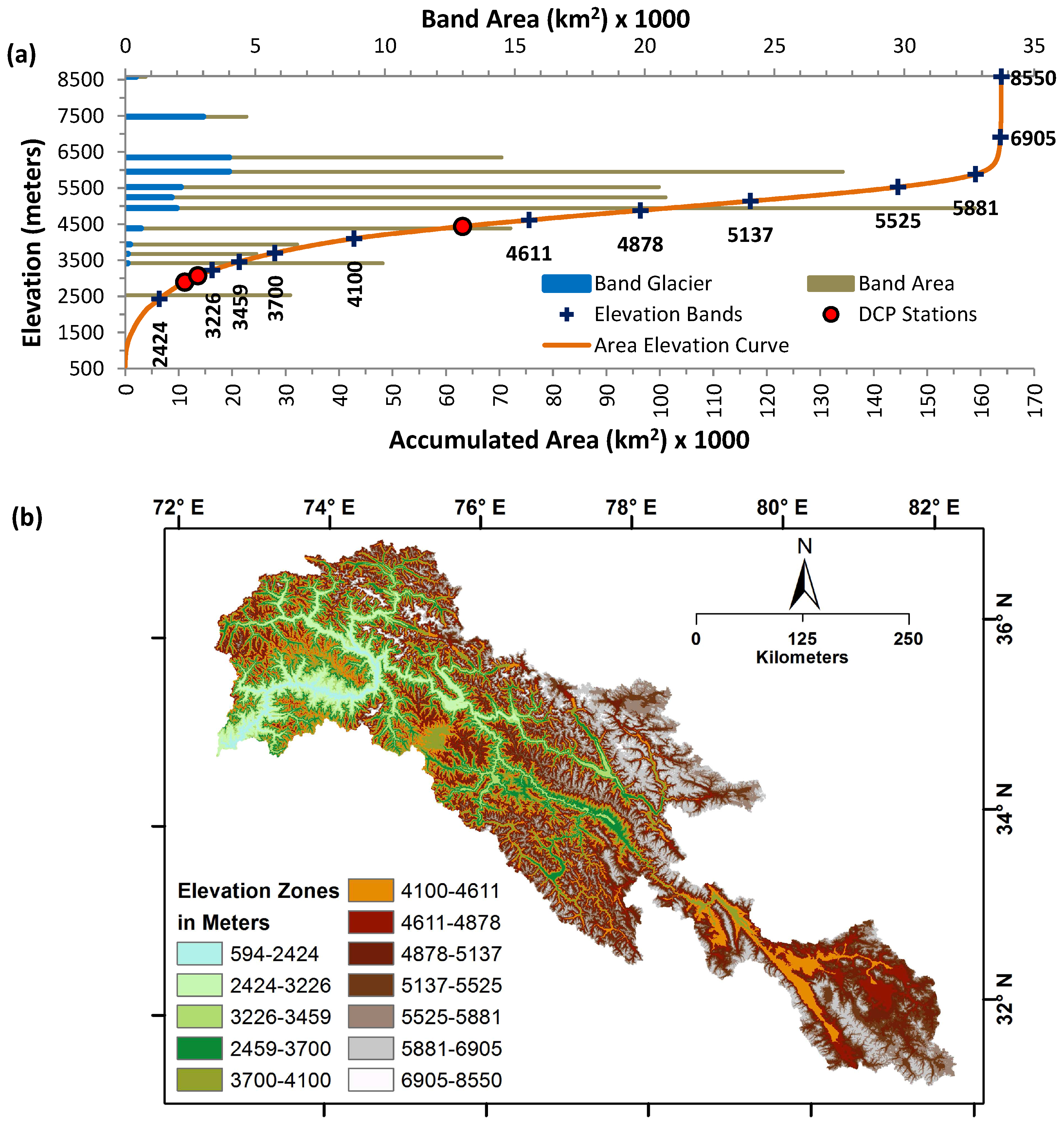
2. Study Area
3. Data Used
4. Methods
4.1. Hydrological Model
4.2. Model Setup, Calibration and Validation
4.2.1. Model Setup
4.2.2. Calibration and Validation
4.3. Climate Change Scenarios
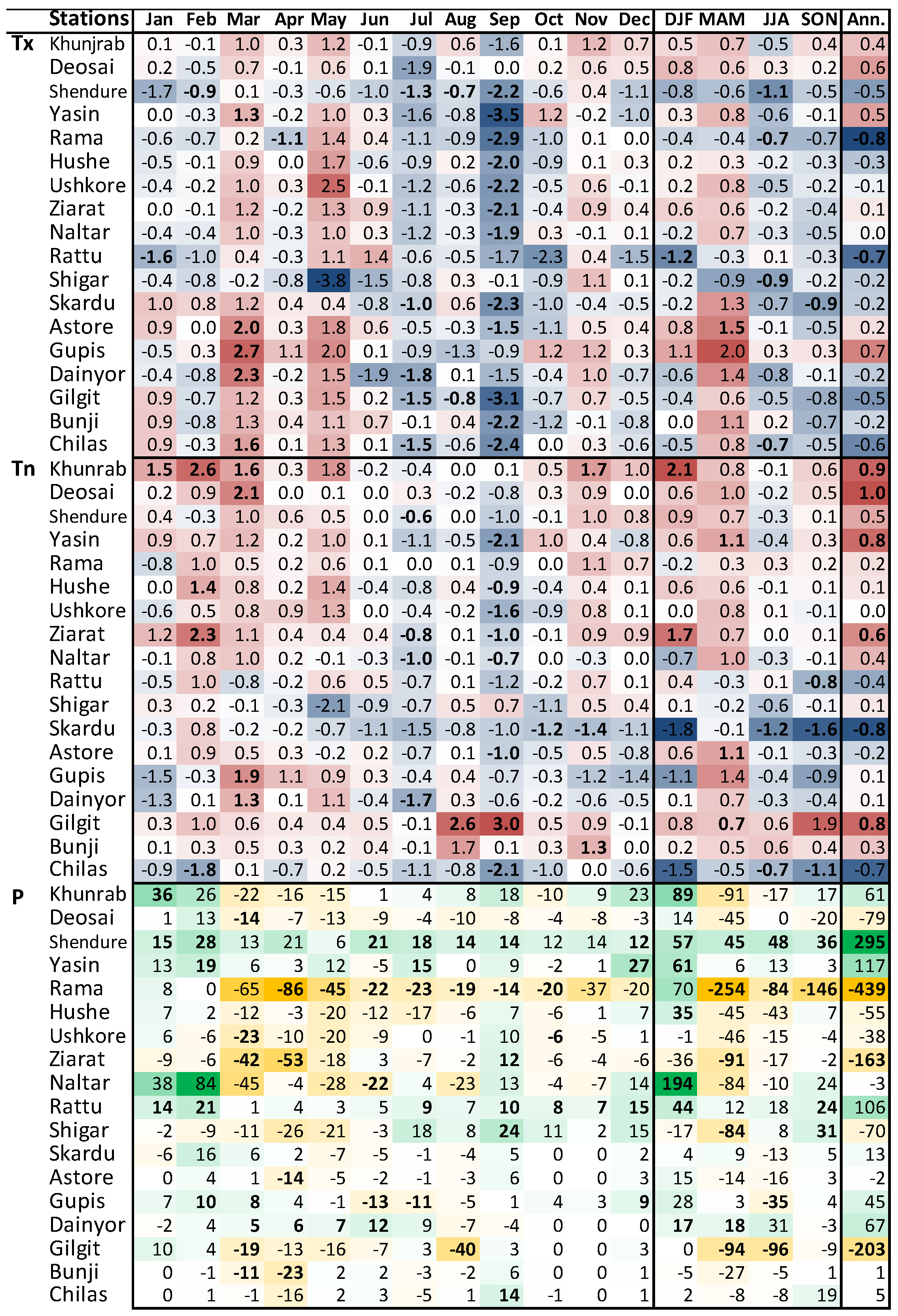
4.3.1. Prevailing Hydro-Cryo-Climatic Changes
4.3.2. Near-Future Climate Change Scenario
4.3.3. Far-Future Climate Change Scenario
5. Results
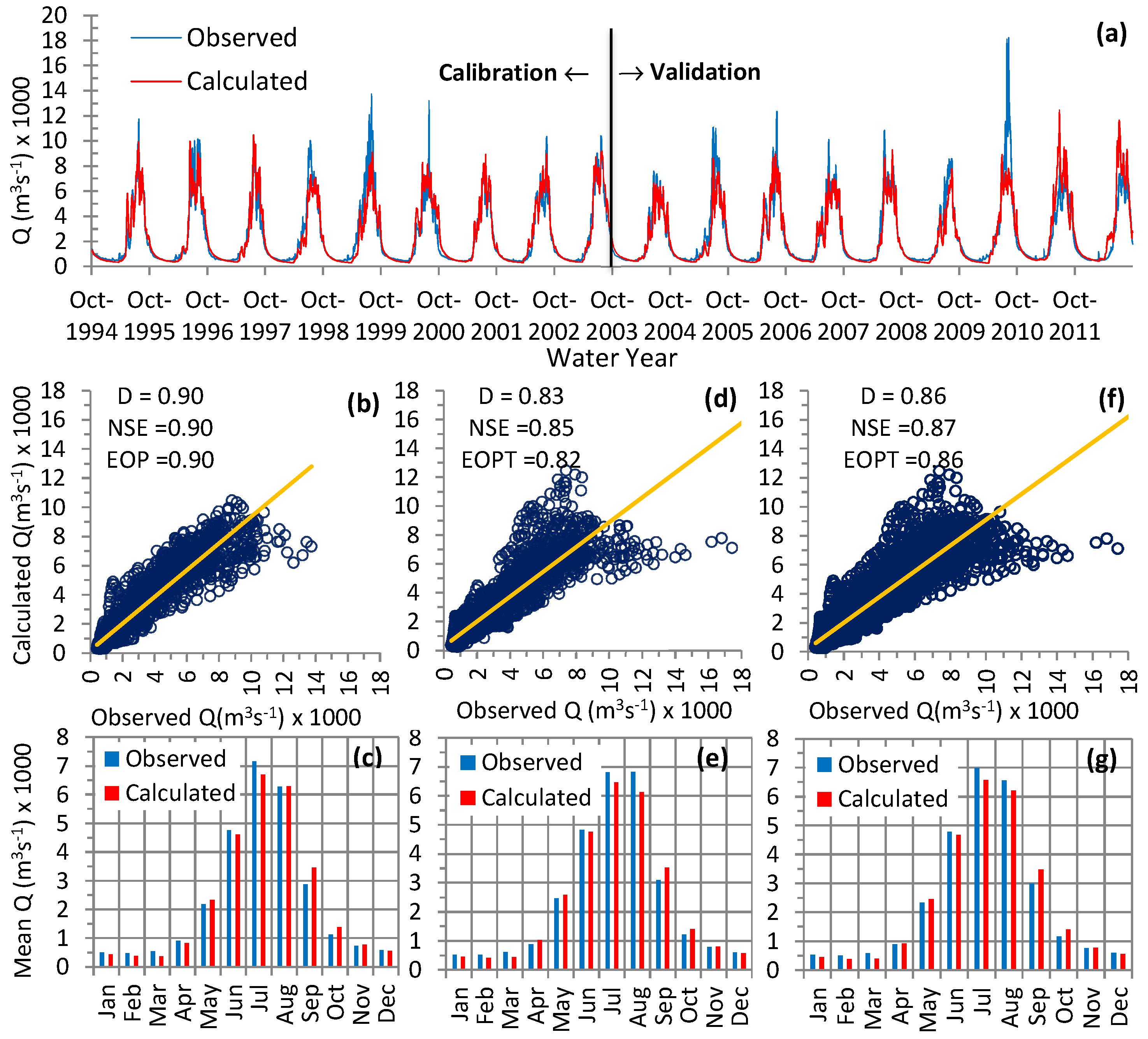
5.1. Calibration and Validation
5.1.1. UBC Model
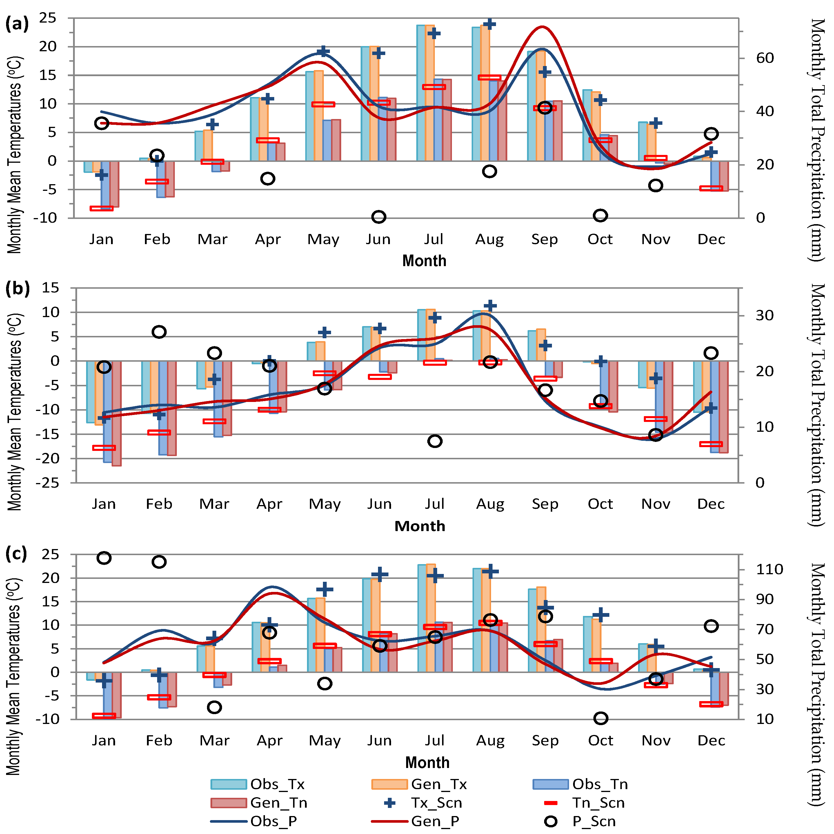
5.1.2. LARS-WG
5.2. Future Water Availability
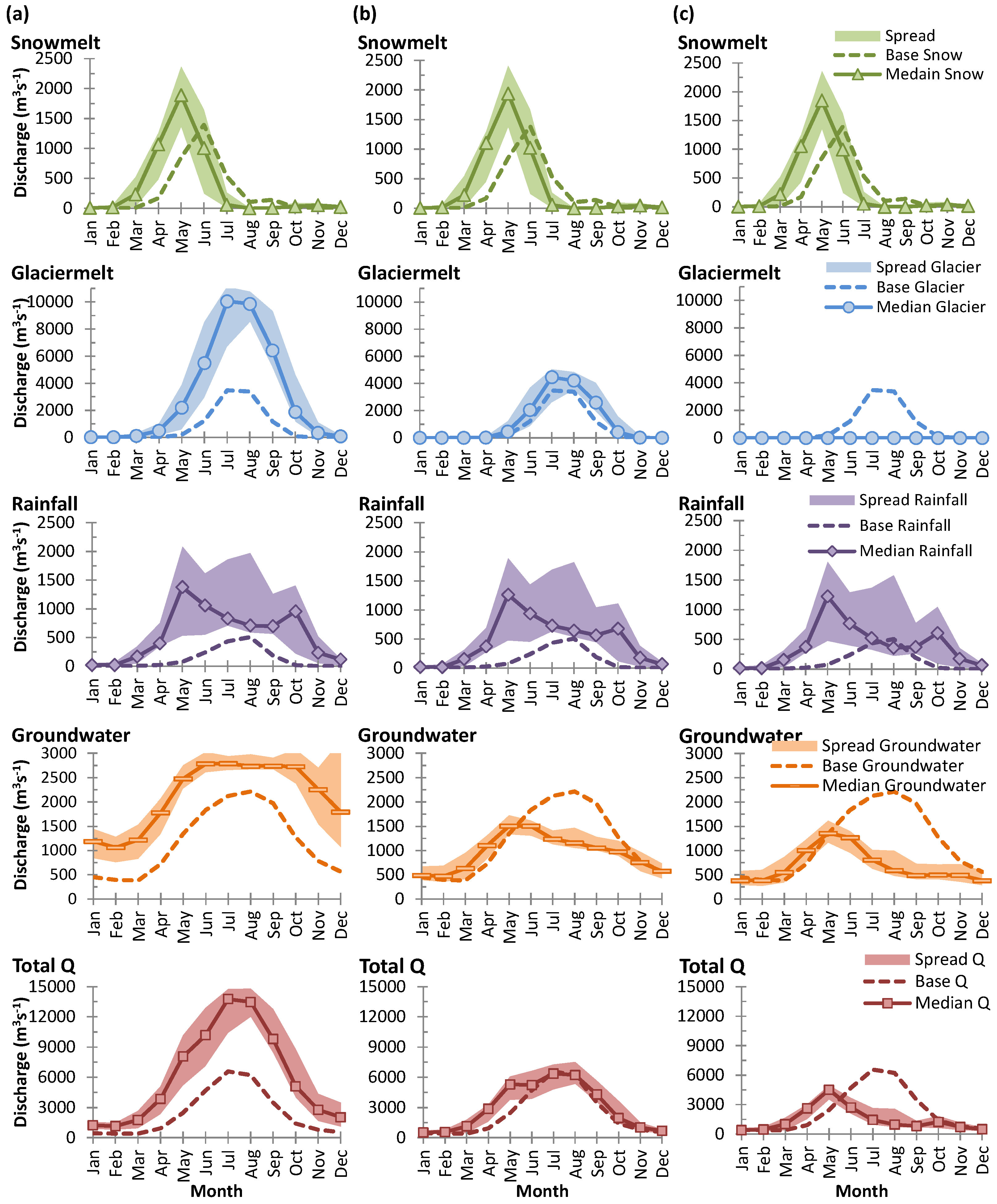
5.2.1. Near-Future Climate Change Scenarios
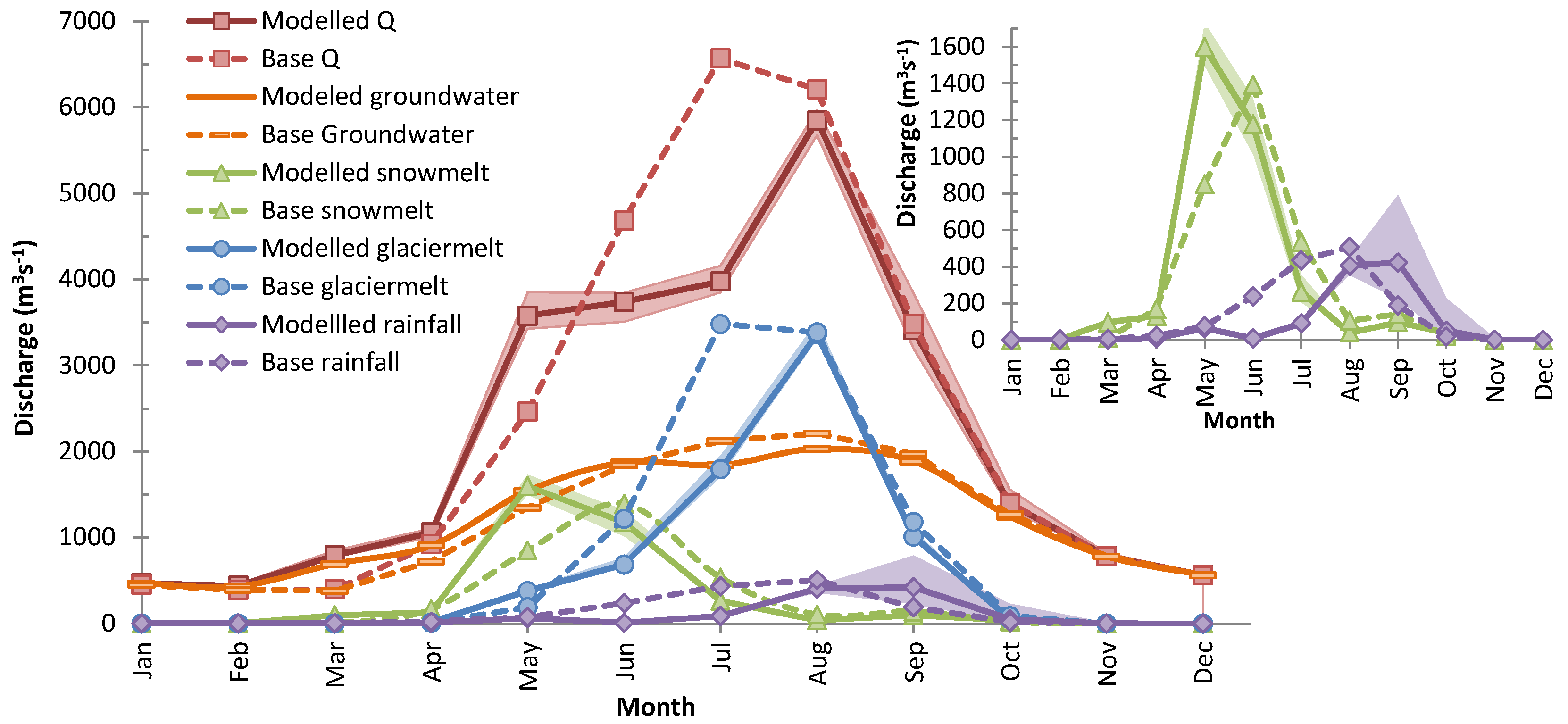
5.2.2. Far-Future Climate Change Scenario (Intact Glacier)
5.2.3. Far-Future Climate Change Scenario (50% Glacier)
5.2.4. Far-Future Climate Change Scenario (No Glacier)
6. Discussion
7. Conclusions
Acknowledgments
Author Contributions
Conflicts of Interest
Abbreviations
| UIB | Upper Indus Basin |
| HKH | Hindukush-Karakoram-Himalaya |
| UBC | University of British Columbia |
| AEC | Area Elevation Curve |
| DEM | Digital Elevation Model |
| MODIS | MODerate Resolution Imaging Spectroradiometer |
| CORDEX-SA | Coordinated Regional Climate Downscaling Experiments for South Asia |
Appendix A UBC Snowmelt Routine and Snowpack Budget
References
- IPCC. Climate Change 2013: The Physical Science Basis. Contribution of Working Group I to the Fifth Assessment Report of The Intergovernmental Panel on Climate Change; IPCC: New York, NY, USA, 2013. [Google Scholar]
- MRI. Elevation-dependent warming in mountain regions of the world. Nat. Clim. Chang. 2015, 5, 424–430. [Google Scholar]
- Hasson, S.; Gerlitz, L.; Schickhoff, U.; Scholten, T.; Böhner, J. Recent climate change over high Asia. In Climate Change, Glacier Response, and Vegetation Dynamics in the Himalaya; Springer: Basel, Switzerland, 2016; pp. 199–217. [Google Scholar]
- Hasson, S.; Böhner, J.; Lucarini, V. Prevailing climatic trends and runoff response from Hindukush- Karakoram-Himalaya, upper Indus basin. Earth Syst. Dyn. Discuss. 2015, 6, 579–653. [Google Scholar] [CrossRef]
- Immerzeel, W.W.; Droogers, P.; de Jong, S.; Bierkens, M. Large-scale monitoring of snow cover and runoff simulation in Himalayan river basins using remote sensing. Remote Sens. Environ. 2009, 113, 40–49. [Google Scholar] [CrossRef]
- Lutz, A.; Immerzeel, W.; Shrestha, A.; Bierkens, M. Consistent increase in High Asia’s runoff due to increasing glacier melt and precipitation. Nat. Clim. Chang. 2014, 4, 587–592. [Google Scholar] [CrossRef]
- Ali, S.; Li, D.; Congbin, F.; Khan, F. Twenty first century climatic and hydrological changes over Upper Indus Basin of Himalayan region of Pakistan. Environ. Res. Lett. 2015, 10, 014007. [Google Scholar] [CrossRef]
- Khan, F.; Pilz, J.; Amjad, M.; Wiberg, D.A. Climate variability and its impacts on water resources in the Upper Indus Basin under IPCC climate change scenarios. Int. J. Glob. Warm. 2015, 8, 46–69. [Google Scholar] [CrossRef]
- Akhtar, M.; Ahmad, N.; Booij, M. The impact of climate change on the water resources of Hindukush- Karakorum-Himalaya region under different glacier coverage scenarios. J. Hydrol. 2008, 355, 148–163. [Google Scholar] [CrossRef]
- Tahir, A.A.; Chevallier, P.; Arnaud, Y.; Neppel, L.; Ahmad, B. Modeling snowmelt-runoff under climate scenarios in the Hunza River basin, Karakoram Range, Northern Pakistan. J. Hydrol. 2011, 409, 104–117. [Google Scholar] [CrossRef]
- Bocchiola, D.; Diolaiuti, G.; Soncini, A.; Mihalcea, C.; D’Agata, C.; Mayer, C.; Lambrecht, A.; Rosso, R.; Smiraglia, C. Prediction of future hydrological regimes in poorly gauged high altitude basins: The case study of the upper Indus, Pakistan. Hydrol. Earth Syst. Sci. 2011, 15, 2059–2075. [Google Scholar] [CrossRef]
- Naeem, U.A.; Hashmi, H.N.; Shamim, M.; Ejaz, N. Flow variations in Astore River under assumed glaciated extents due to climate change. Pak. J. Eng. Appl. Sci. 2012, 11, 73–81. [Google Scholar]
- Immerzeel, W.; Pellicciotti, F.; Bierkens, M. Rising river flows throughout the twenty-first century in two Himalayan glacierized watersheds. Nat. Geosci. 2013, 6, 742–745. [Google Scholar] [CrossRef]
- Soncini, A.; Bocchiola, D.; Confortola, G.; Bianchi, A.; Rosso, R.; Mayer, C.; Lambrecht, A.; Palazzi, E.; Smiraglia, C.; Diolaiuti, G. Future hydrological regimes in the Upper Indus Basin: A case study from a high-altitude glacierized catchment. J. Hydrometeorol. 2015, 16, 306–326. [Google Scholar] [CrossRef]
- Mishra, V. Climatic uncertainty in Himalayan water towers. J. Geophys. Res. Atmos. 2015, 120, 2689–2705. [Google Scholar] [CrossRef]
- Hasson, S.; Böhner, J.; Chishtie, F. Low fidelity of present-day climate modelling experiments and future climatic uncertainty over Himalayan watersheds of Indus basin. Clim. Dyn. 2016. under review. [Google Scholar]
- Fowler, H.; Archer, D. Conflicting signals of climatic change in the Upper Indus Basin. J. Clim. 2006, 19, 4276–4293. [Google Scholar] [CrossRef]
- Sheikh, M.; Manzoor, N.; Adnan, M.; Ashraf, J.; Khan, A.M. Climate Profile and Past Climate Changes in Pakistan; GCISC Report No. RR-01; Global Change Impact Studies Centre (GCISC): Islamabad, Pakistan, 2009. [Google Scholar]
- Khattak, M.S.; Babel, M.; Sharif, M. Hydro-meteorological trends in the upper Indus River basin in Pakistan. Clim. Res. 2011, 46, 103–119. [Google Scholar] [CrossRef]
- Minora, U.; Bocchiola, D.; D’Agata, C.; Maragno, D.; Mayer, C.; Lambrecht, A.; Mosconi, B.; Vuillermoz, E.; Senese, A.; Compostella, C.; et al. 2001–2010 glacier changes in the Central Karakoram National Park: A contribution to evaluate the magnitude and rate of the “Karakoram anomaly”. Cryosphere Discuss. 2013, 7, 2891–2941. [Google Scholar] [CrossRef]
- Bocchiola, D.; Diolaiuti, G. Recent (1980–2009) evidence of climate change in the upper Karakoram, Pakistan. Theor. Appl. Climatol. 2013, 113, 611–641. [Google Scholar] [CrossRef]
- Minora, U.; Bocchiola, D.; D’Agata, C.; Diolaiuti, G.; Mayer, C.; Lambrecht, A.; Vuillermoz, A.; Senese, A.; Compostella, C.; Smiraglia, C. Glacier area stability in the Central Karakoram National Park (Pakistan) in 2001–2010: The “Karakoram Anomaly” in the spotlight. Prog. Phys. Geogr. 2013. [Google Scholar] [CrossRef]
- Zafar, M.U.; Ahmed, M.; Rao, M.P.; Buckley, B.M.; Khan, N.; Wahab, M.; Palmer, J. Karakorum temperature out of phase with hemispheric trends for the past five centuries. Clim. Dyn. 2015, 46, 1943–1952. [Google Scholar] [CrossRef]
- Archer, D.R.; Fowler, H.J. Spatial and temporal variations in precipitation in the Upper Indus Basin, global teleconnections and hydrological implications. Hydrol. Earth Syst. Sci. 2004, 8, 47–61. [Google Scholar] [CrossRef]
- Hasson, S.; Lucarini, V.; Khan, M.; Petitta, M.; Bolch, T.; Gioli, G. Early 21st century snow cover state over the western river basins of the Indus River system. Hydrol. Earth Syst. Sci. 2014, 18, 4077–4100. [Google Scholar] [CrossRef]
- Tahir, A.A.; Adamowski, J.F.; Chevallier, P.; Haq, A.U.; Terzago, S. Comparative assessment of spatiotemporal snow cover changes and hydrological behavior of the Gilgit, Astore and Hunza River basins (Hindukush- Karakoram-Himalaya region, Pakistan). Meteorol. Atmos. Phys. 2016. [Google Scholar] [CrossRef]
- Hewitt, K. The Karakoram anomaly? Glacier expansion and the ‘elevation effect’, Karakoram Himalaya. Mt. Res. Dev. 2005, 25, 332–340. [Google Scholar] [CrossRef]
- Scherler, D.; Bookhagen, B.; Strecker, M.R. Spatially variable response of Himalayan glaciers to climate change affected by debris cover. Nat. Geosci. 2011, 4, 156–159. [Google Scholar] [CrossRef]
- Bhambri, R.; Bolch, T.; Kawishwar, P.; Dobhal, D.; Srivastava, D.; Pratap, B. Heterogeneity in glacier response in the upper Shyok valley, northeast Karakoram. Cryosphere 2013, 7, 1385–1398. [Google Scholar] [CrossRef]
- Rankl, M.; Kienholz, C.; Braun, M. Glacier changes in the Karakoram region mapped by multimission satellite imagery. Cryosphere 2014, 8, 977–989. [Google Scholar] [CrossRef]
- Hewitt, K. Glacier change, concentration, and elevation effects in the Karakoram Himalaya, Upper Indus Basin. Mt. Res. Dev. 2011, 31, 188–200. [Google Scholar] [CrossRef]
- Gardelle, J.; Berthier, E.; Arnaud, Y. Slight mass gain of Karakoram glaciers in the early twenty-first century. Nat. Geosci. 2012, 5, 322–325. [Google Scholar] [CrossRef]
- Gardelle, J.; Berthier, E.; Arnaud, Y.; Kaab, A. Region-wide glacier mass balances over the Pamir- Karakoram-Himalaya during 1999–2011. Cryosphere 2013, 7, 1885–1886. [Google Scholar] [CrossRef]
- Kaab, A.; Berthier, E.; Nuth, C.; Gardelle, J.; Arnaud, Y. Contrasting patterns of early twenty-first-century glacier mass change in the Himalayas. Nature 2012, 488, 495–498. [Google Scholar] [CrossRef] [PubMed]
- Kääb, A.; Treichler, D.; Nuth, C.; Berthier, E. Brief communication: Contending estimates of 2003–2008 glacier mass balance over the Pamir-Karakoram-Himalaya. Cryosphere 2015, 9, 557–564. [Google Scholar] [CrossRef]
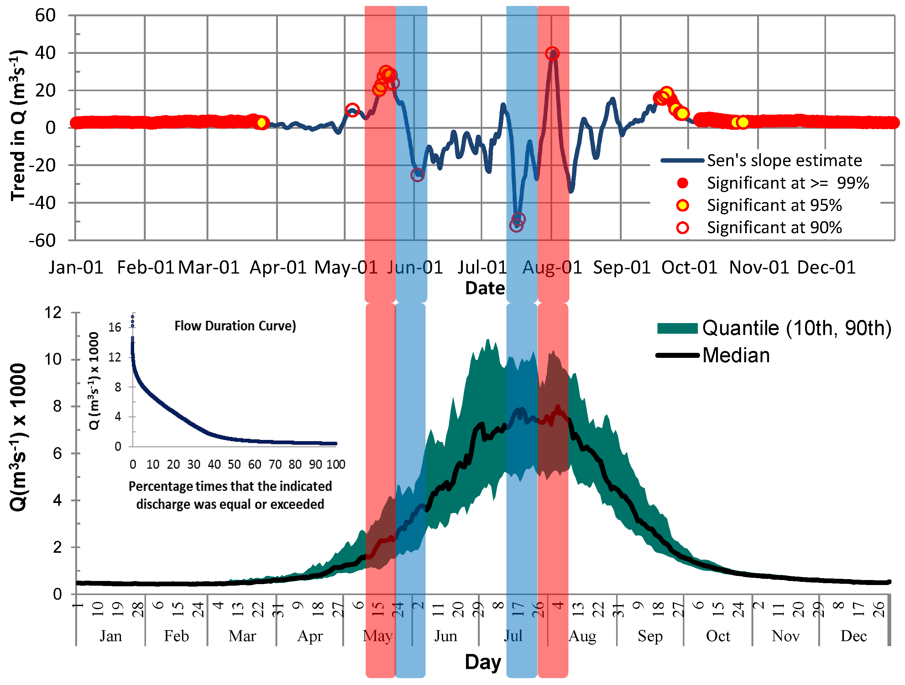
- Sharif, M.; Archer, D.R.; Fowler, H.J.; Forsythe, N. Trends in timing and magnitude of flow in the Upper Indus Basin. Hydrol. Earth Syst. Sci. 2013, 17, 1503–1516. [Google Scholar] [CrossRef]
- Wi, S.; Yang, Y.; Steinschneider, S.; Khalil, A.; Brown, C. Calibration approaches for distributed hydrologic models in poorly gaged basins: Implication for streamflow projections under climate change. Hydrol. Earth Syst. Sci. 2015, 19, 857–876. [Google Scholar] [CrossRef]
- Quick, M.C.; Pipes, A. A combined snowmelt and rainfall runoff model. Can. J. Civ. Eng. 1976, 3, 449–460. [Google Scholar] [CrossRef]
- Arendt, A.; Bliss, A.; Bolch, T.; Cogley, J.G.; Gardner, A.S.; Hagen, J.-O.; Hock, R.; Huss, M.; Kaser, G.; Kienholz, C.; et al. Randolph Glacier Inventory—A Dataset of Global Glacier Outlines, 5th ed.; Global Land Ice Measurements from Space; Digital Media: Boulder, CO, USA, 2015. [Google Scholar]
- Krasovskaia, I.; Arnell, N.; Gottschalk, L. Flow regimes in northern and western Europe: Development and application of procedures for classifying flow regimes. IAHS Publ. 1994, 221, 185–192. [Google Scholar]
- SIHP. Snow and Ice Hydrology; Pakistan Phase-II Final Report to CIDA, IDRC File No.88-8009-00; International Development Research Centre: Ottawa, ON, Canada, 1997. [Google Scholar]
- Archer, D. Contrasting hydrological regimes in the upper Indus Basin. J. Hydrol. 2003, 274, 198–210. [Google Scholar] [CrossRef]
- Wake, C.P. Glaciochemical investigations as a tool for determining the spatial and seasonal variation of snow accumulation in the central Karakoram, northern Pakistan. Ann. Glaciol. 1989, 13, 279–284. [Google Scholar]
- Ali, G.; Hasson, S.; Khan, A.M. Climate Change: Implications and Adaptation of Water Resources in Pakistan; Technical Report GCISC-RR-13; Global Change Impact Studies Centre (GCISC): Islamabad, Pakistan, 2009. [Google Scholar]
- Palazzi, E.; Hardenberg, J.; Provenzale, A. Precipitation in the Hindu-Kush Karakoram Himalaya: Observations and future scenarios. J. Geophys. Res. Atmos. 2013, 118, 85–100. [Google Scholar] [CrossRef]
- Hasson, S.; Lucarini, V.; Pascale, S.; Böhner, J. Seasonality of the hydrological cycle in major South and Southeast Asian river basins as simulated by PCMDI/CMIP3 experiments. Earth Syst. Dyn. 2014, 5, 67–87. [Google Scholar] [CrossRef]
- Hasson, S.; Pascale, S.; Lucarini, V.; Böhner, J. Seasonal cycle of precipitation over major river basins in South and Southeast Asia: A review of the {CMIP5} climate models data for present climate and future climate projections. Atmos. Res. 2016, 180, 42–63. [Google Scholar] [CrossRef]
- Shaman, J.; Tziperman, E. The effect of ENSO on Tibetan Plateau snow depth: A stationary wave teleconnection mechanism and implications for the South Asian monsoons. J. Clim. 2005, 18, 2067–2079. [Google Scholar] [CrossRef]
- Syed, F.; Giorgi, F.; Pal, J.; King, M. Effect of remote forcings on the winter precipitation of central southwest Asia part 1: Observations. Theor. Appl. Climatol. 2006, 86, 147–160. [Google Scholar] [CrossRef]
- UNEP. As Compiled from USGS/NASA—Distributed Active Archive Center; United Nations Environment Programme: Geneva, Switzerland, 2015. [Google Scholar]
- Pipes, A.; Quick, M.C. Modelling large scale effects of snow cover. In Large Scale Effects of Seasonal Snow Cover; International Association of Hydrological Sciences Press & Institute of Hydrology: Wallingford, UK, 1987; pp. 151–160. [Google Scholar]
- Loukas, A.; Vasiliades, L.; Dalezios, N.R. Potential climate change impacts on flood producing mechanisms in southern British Columbia, Canada using the CGCMA1 simulation results. J. Hydrol. 2002, 259, 163–188. [Google Scholar] [CrossRef]
- Loukas, A.; Vasiliades, L. Streamflow simulation methods for ungauged and poorly gauged watersheds. Nat. Hazards Earth Syst. Sci. 2014, 14, 1641–1661. [Google Scholar] [CrossRef]
- Huntington, E. Pangong: A glacial lake in the Tibetan Plateau. J. Geol. 1906, 14, 599–617. [Google Scholar] [CrossRef]
- Brown, E.; Bendick, R.; Bourles, D.; Gaur, V.; Molnar, P.; Raisbeck, G.; Yiou, F. Early Holocene climate recorded in geomorphological features in Western Tibet. Palaeogeogr. Palaeoclimatol. Palaeoecol. 2003, 199, 141–151. [Google Scholar] [CrossRef]
- Hasson, S. Atypical uncertainties in modelling runoff from Hindukush-Karakoram-Himalaya, upper Indus basin. 2016; in preparation. [Google Scholar]
- Mayer, C.; Lambrecht, A.; Mihalcea, C.; Belò, M.; Diolaiuti, G.; Smiraglia, C.; Bashir, F. Analysis of glacial meltwater in Bagrot Valley, Karakoram: Based on short-term ablation and debris cover observations on Hinarche Glacier. Mt. Res. Dev. 2010, 30, 169–177. [Google Scholar] [CrossRef]
- Winiger, M.; Gumpert, M.; Yamout, H. Karakorum-Hindukush-western Himalaya: Assessing high-altitude water resources. Hydrol. Process. 2005, 19, 2329–2338. [Google Scholar] [CrossRef]
- Young, G.; Schmok, J. Ice loss in the ablation area of a Himalayan glacier: Studies on Miar Glacier, Karakorum Mountains, Pakistan. Ann. Glaciol. 1989, 13, 289–293. [Google Scholar]
- Young, G.; Hewitt, K. Hydrology research in the upper Indus basin, Karakoram Himalaya, Pakistan. Hydrol. Mt. Areas 1990, 190, 139–152. [Google Scholar]
- Hewitt, K. Tributary glacier surges: An exceptional concentration at Panmah Glacier, Karakoram Himalaya. J. Glaciol. 2007, 53, 181–188. [Google Scholar] [CrossRef]
- Tahir, A.A.; Chevallier, P.; Arnaud, Y.; Ashraf, M.; Bhatti, M.T. Snow cover trend and hydrological characteristics of the Astore River basin (Western Himalayas) and its comparison to the Hunza basin (Karakoram region). Sci. Total Environ. 2015, 505, 748–761. [Google Scholar] [CrossRef] [PubMed]
- Immerzeel, W.W.; Pellicciotti, F.; Shrestha, A.B. Glaciers as a proxy to quantify the spatial distribution of precipitation in the Hunza basin. Mt. Res. Dev. 2012, 32, 30–38. [Google Scholar] [CrossRef]
- Pratap, B.; Dobhal, D.; Mehta, M.; Bhambri, R. Influence of debris cover and altitude on glacier surface melting: A case study on Dokriani Glacier, central Himalaya, India. Ann. Glaciol. 2015, 56, 9–16. [Google Scholar] [CrossRef]
- Bolch, T.; Kulkarni, A.; Kääb, A.; Huggel, C.; Paul, F.; Cogley, J.; Frey, H.; Kargel, J.S.; Fujita, K.; Scheel, M.; et al. The state and fate of Himalayan glaciers. Science 2012, 336, 310–314. [Google Scholar] [CrossRef] [PubMed]
- Mihalcea, C.; Mayer, C.; Diolaiuti, G.; D’agata, C.; Smiraglia, C.; Lambrecht, A.; Vuillermoz, E.; Tartari, G. Spatial distribution of debris thickness and melting from remote-sensing and meteorological data, at debris-covered Baltoro glacier, Karakoram, Pakistan. Ann. Glaciol. 2008, 48, 49–57. [Google Scholar] [CrossRef]
- Minora, U.; Senese, A.; Bocchiola, D.; Soncini, A.; D’Agata, C.; Ambrosini, R.; Mayer, C.; Lambrecht, A.; Vuillermoz, E.; Smiraglia, C.; et al. A simple model to evaluate ice melt over the ablation area of glaciers in the Central Karakoram National Park, Pakistan. Ann. Glaciol. 2015, 56, 202–216. [Google Scholar] [CrossRef]
- Bajracharya, S.R.; Maharjan, S.B.; Shrestha, F.; Guo, W.; Liu, S.; Immerzeel, W.; Shrestha, B. The glaciers of the Hindu Kush Himalayas: Current status and observed changes from the 1980s to 2010. Int. J. Water Resour. Dev. 2015, 31, 161–173. [Google Scholar] [CrossRef]
- Herreid, S.; Pellicciotti, F.; Ayala, A.; Chesnokova, A.; Kienholz, C.; Shea, J.; Shrestha, A. Satellite observations show no net change in the percentage of supraglacial debris-covered area in northern Pakistan from 1977 to 2014. J. Glaciol. 2015, 61, 524–536. [Google Scholar] [CrossRef]
- SIHP. Snow and Ice Hydrology Project; Technical Report IDRC File No. 88-8009-00; Water and Power Development Authority (WAPDA), Hydrology and Research Directorate: Lahore, Pakistan, 1986. [Google Scholar]
- Mattson, L. Ablation on debris covered glaciers: An example from the Rakhiot Glacier, Panjab, Himalaya. IAHS Publ. 1993, 218, 289–296. [Google Scholar]
- Mihalcea, C.; Mayer, C.; Diolaiuti, G.; Lambrecht, A.; Smiraglia, C.; Tartari, G. Ice ablation and meteorological conditions on the debris-covered area of Baltoro glacier, Karakoram, Pakistan. Ann. Glaciol. 2006, 43, 292–300. [Google Scholar] [CrossRef]
- Krause, P.; Boyle, D.; Bäse, F. Comparison of different efficiency criteria for hydrological model assessment. Adv. Geosci. 2005, 5, 89–97. [Google Scholar] [CrossRef]
- Nash, J.E.; Sutcliffe, J.V. River flow forecasting through conceptual models part I—A discussion of principles. J. Hydrol. 1970, 10, 282–290. [Google Scholar] [CrossRef]
- Mukhopadhyay, B.; Khan, A.; Gautam, R. Rising and falling river flows: Contrasting signals of climate change and glacier mass balance from the eastern and western Karakoram. Hydrol. Sci. J. 2015, 60, 2062–2085. [Google Scholar] [CrossRef]
- Gioli, G.; Khan, T.; Scheffran, J. Climatic and environmental change in the Karakoram: Making sense of community perceptions and adaptation strategies. Reg. Environ. Chang. 2014, 14, 1151–1162. [Google Scholar] [CrossRef]
- Theil, H. A rank-invariant method of linear and polynomial regression analysis. In Collection of Henri Theil’s Contributions to Economics and Econometrics; Springer: Basel, Switzerland, 1992; pp. 345–381. [Google Scholar]
- Sen, P.K. Estimates of the regression coefficient based on Kendall’s tau. J. Am. Stat. Assoc. 1968, 63, 1379–1389. [Google Scholar] [CrossRef]
- Semenov, M.A.; Pilkington-Bennett, S.; Calanca, P. Validation of ELPIS 1980-2010 baseline scenarios using the observed European Climate Assessment data set. Clim. Res. 2013, 57, 1–9. [Google Scholar] [CrossRef]
- Moss, R.H.; Edmonds, J.A.; Hibbard, K.A.; Manning, M.R.; Rose, S.K.; van Vuuren, D.P.; Carter, T.R.; Emori, S.; Kainuma, M.; Kram, T.; et al. The next generation of scenarios for climate change research and assessment. Nature 2010, 463, 747–756. [Google Scholar] [CrossRef] [PubMed]
- Van Vuuren, D.P.; Edmonds, J.; Kainuma, M.; Riahi, K.; Thomson, A.; Hibbard, K.; Hurtt, G.C.; Kram, T.; Krey, V.; Lamarque, J.F.; et al. The representative concentration pathways: An overview. Clim. Chang. 2011, 109, 5–31. [Google Scholar] [CrossRef]
- Islam, S.; Rehman, N.; Sheikh, M.M.; Khan, A.M. High Resolution Climate Change Scenarios over South Asia Region Donscaled by Regional Climate Model PRECIS for IPCC SRES A2 Scneario; Technical Report GCISC-RR-06; Global Change Impact Studies Centre (GCISC): Islamabad, Pakistan, 2009. [Google Scholar]
- Kulkarni, A.; Patwardhan, S.; Kumar, K.K.; Ashok, K.; Krishnan, R. Projected climate change in the Hindu Kush-Himalayan region by using the high-resolution regional climate model PRECIS. Mt. Res. Dev. 2013, 33, 142–151. [Google Scholar] [CrossRef]
- Syed, F.S.; Iqbal, W.; Syed, A.A.B.; Rasul, G. Uncertainties in the regional climate models simulations of South-Asian summer monsoon and climate change. Clim. Dyn. 2014, 42, 2079–2097. [Google Scholar] [CrossRef]
- Rajbhandari, R.; Shrestha, A.; Kulkarni, A.; Patwardhan, S.; Bajracharya, S. Projected changes in climate over the Indus river basin using a high resolution regional climate model (PRECIS). Clim. Dyn. 2015, 44, 339–357. [Google Scholar] [CrossRef]
- Iqbal, W.; Syed, F.; Sajjad, H.; Nikulin, G.; Kjellström, E.; Hannachi, A. Mean climate and representation of jet streams in the CORDEX South Asia simulations by the regional climate model RCA4. Theor. Appl. Climatol. 2016. [Google Scholar] [CrossRef]
- Hasson, S. Seasonality of Precipitation over Himalayan Watersheds in CORDEX South Asia and their CMIP5 forcing experiments. Atmosphere 2016. under review. [Google Scholar]
- Hasson, S.; Lucarini, V.; Pascale, S. Hydrological cycle over South and Southeast Asian river basins as simulated by PCMDI/CMIP3 experiments. Earth Syst. Dyn. 2013, 4, 199–217. [Google Scholar] [CrossRef]
- Finger, D.; Vis, M.; Huss, M.; Seibert, J. The value of multiple data set calibration versus model complexity for improving the performance of hydrological models in mountain catchments. Water Resour. Res. 2015, 51, 1939–1958. [Google Scholar] [CrossRef]
- Rees, G.; Collins, D. An Assessment of the Potential Impacts of Deglaciation on the Water Resources of the Himalaya; Technical Report R7890; Centre for for Ecology and Hydrology: Oxfordshire, UK, 2004. [Google Scholar]
- Singh, P.; Kumar, N. Impact assessment of climate change on the hydrological response of a snow and glacier melt runoff dominated Himalayan river. J. Hydrol. 1997, 193, 316–350. [Google Scholar] [CrossRef]
- Kundzewicz, Z.W.; Gerten, D. Grand challenges related to the assessment of climate change impacts on freshwater resources. J. Hydrol. Eng. 2014, 20, A4014011. [Google Scholar] [CrossRef]


| S. No. | Station Name | From | To | Agency | Latitude | Longitude | Height (m) | Basin |
|---|---|---|---|---|---|---|---|---|
| Meteorological Stations | ||||||||
| 1. | Khunjrab | 1995 | 2012 | WAPDA | 36.841110 | 75.419170 | 4440 | Hunza |
| 2. | Naltar | 1995 | 2012 | WAPDA | 36.166670 | 74.183000 | 2898 | Hunza |
| 3. | Hushe | 1995 | 2012 | WAPDA | 35.423890 | 76.367000 | 3075 | Shyok |
| Discharge Station | ||||||||
| 1. | Besham Qila | 1969 | 2012 | WAPDA | 34.924167 | 75.381944 | 580 | UIB |
| S. No. | Experiment Name | Forcing GCM | RCM Employed |
|---|---|---|---|
| 1 | ACCESS1-0_CCAM | ACCESS1-0 | CCAM—Conformal-Cubic Atmospheric Model from Commonwealth Scientific and Industrial Research Organization |
| 2 | CCSM4_CCAM | CCSM4 | CCAM |
| 3 | CNRM-CM5_CCAM | CNRM-CM5 | CCAM |
| 4 | GFDL-CM3_CCAM | GFDL-CM3 | CCAM |
| 5 | MPI-ESM-LR_CCAM | MPI-ESM-LR | CCAM |
| 6 | EC-EARTH_RCA4 | EC-EARTH | RCA4—Rossby Centre regional atmospheric model version 4-2 |
| 7 | MPI-ESM-LR_REMOi | MPI-ESM-LR | REMO—The Regional Model for climate simulations was jointly developed by Max Plank Institute for Meteorology (MPI-M) and German Climate Computing Centre (DKRZ) |
| Parameters | Elevation Bands | |||||||||||
|---|---|---|---|---|---|---|---|---|---|---|---|---|
| 1 | 2 | 3 | 4 | 5 | 6 | 7 | 8 | 9 | 10 | 11 | 12 | |
| Mid-elevation (meters) | 1902 | 2884 | 3347 | 3584 | 3914 | 4373 | 4746 | 5008 | 5321 | 5678 | 6092 | 7180 |
| Area (km) | 5840 | 9765 | 5016 | 6565 | 14,793 | 32,837 | 21,324 | 20,995 | 28,206 | 14,986 | 4840 | 149 |
| Forested fraction | 0.15 | 0.08 | 0.04 | 0.02 | 0.01 | 0.00 | 0.00 | 0.00 | 0.00 | 0.00 | 0.00 | 0.00 |
| Forest canopy density | 0.13 | 0.08 | 0.38 | 0.03 | 0.01 | 0.00 | 0.00 | 0.00 | 0.00 | 0.00 | 0.00 | 0.00 |
| Orientation index | ||||||||||||
| (0 = North,1 = South) | 0.89 | 0.91 | 0.89 | 0.90 | 0.90 | 0.98 | 0.98 | 0.90 | 0.98 | 0.87 | 0.89 | 0.00 |
| Glacier cover (km) | ||||||||||||
| RGI5 Actual | 0.3 | 102.5 | 111.1 | 194.9 | 639.6 | 1980.3 | 1917.7 | 2402.7 | 4533.3 | 4158.8 | 3171.9 | 157.0 |
| For debris-cover ablation | 0.2 | 51.3 | 55.5 | 97.4 | 319.8 | 1536.0 | 1917.7 | 2402.7 | 4533.3 | 4158.8 | 3171.9 | 157.0 |
| South-oriented | ||||||||||||
| glaciated fraction | 0.94 | 0.89 | 0.95 | 0.95 | 0.94 | 0.94 | 0.96 | 0.95 | 0.94 | 0.94 | 0.95 | 0.96 |
| Change Factors | Variable | Jan | Feb | Mar | Apr | May | Jun | Jul | Aug | Sep | Oct | Nov | Dec |
|---|---|---|---|---|---|---|---|---|---|---|---|---|---|
| Naltar | Tx | −0.16 | −1.07 | 1.55 | −0.56 | 1.87 | 0.88 | −2.31 | −0.58 | −3.9 | 0.48 | −0.45 | −0.16 |
| Tn | 1.28 | 2.8 | 3.24 | 1.19 | 0.63 | −0.23 | −1.07 | 0.25 | −0.71 | 1 | −0.17 | 0.58 | |
| P | 2.39 | 1.46 | 0.31 | 0.68 | 0.47 | 0.94 | 1.04 | 1.13 | 1.62 | 0.35 | 0.77 | 1.18 | |
| Hushe | Tx | −0.53 | −0.5 | 1.14 | −0.24 | 3.41 | −1.18 | −1.49 | 0.59 | −3.58 | −1.72 | −0.07 | 0.76 |
| Tn | 0.07 | 2.72 | 1.71 | 0.41 | 2.66 | −0.94 | −1.4 | 0.58 | −1.21 | −0.87 | 0.92 | 0.47 | |
| P | 0.92 | 0.62 | −0.08 | 0.31 | −0.11 | 0.01 | −0.09 | 0.45 | 0.66 | 0.04 | 0.66 | 1.36 | |
| Khunjrab | Tx | 0.95 | −0.23 | 1.88 | 0.49 | 1.86 | −0.33 | −1.69 | 1.09 | −3.03 | 0.16 | 1.92 | 0.9 |
| Tn | 2.95 | 4.54 | 3.15 | 0.4 | 2.91 | −1.06 | −0.86 | −0.77 | −0.36 | 0.59 | 2.77 | 1.75 | |
| P | 1.7 | 1.76 | 1.68 | 1.25 | 1 | −0.05 | 0.31 | 0.74 | 1.16 | 1.46 | 1.09 | 1.78 |
| Simulation Period | NSE | VE% | EOPT | D | RMSE (m3·s−1) | |
|---|---|---|---|---|---|---|
| Calibration | October 1994 to September 2003 | 0.9 | −0.01 | 0.9 | 0.9 | 810 |
| Validation | October 2003 to September 2012 | 0.85 | −2.24 | 0.82 | 0.83 | 1027 |
| Overall | October 1994 to September 2012 | 0.87 | −1.15 | 0.86 | 0.86 | 925 |
| Station | Variable | Annual Bias | Absolute RMSE | Relative RMSE |
|---|---|---|---|---|
| Hushe | Tmin | 0.01 | 0.146 | 0.017 |
| Tmax | −0.03 | 0.213 | 0.015 | |
| P | 0.6 | 3.642 | 0.086 | |
| Naltar | Tmin | 0.19 | 0.264 | 0.038 |
| Tmax | −0.05 | 0.243 | 0.018 | |
| P | −0.53 | 5.481 | 0.088 | |
| Khunjrab | Tmin | −0.16 | 0.34 | 0.027 |
| Tmax | 0.02 | 0.23 | 0.029 | |
| P | 0.1 | 1.274 | 0.072 |
| Discharge Components | % Change Near-Future | % Change Far-Future | % Change Far-Future | %Change Far-Future | ||||||||
|---|---|---|---|---|---|---|---|---|---|---|---|---|
| Glacier Cover Intact | Glacier Cover Intact | Glacier Cover (−50%) | No Glacier Cover (−100%) | |||||||||
| Min | Max | Median | Min | Max | Median | Min | Max | Median | Min | Max | Median | |
| Snowmelt | 1.6 | 13.9 | 7 | −2 | 74 | 25 | 1 | 62 | 24 | −4 | 58 | 19 |
| Glacier melt | −20.8 | −25.2 | −23.5 | 166 | 433 | 295 | −4 | 116 | 54 | −100 | −100 | −100 |
| Rainfall | −0.3 | −43.4 | −29.2 | 205 | 520 | 344 | 154 | 442 | 286 | 104 | 366 | 233 |
| Groundwater | −0.2 | 3 | 1.8 | 56 | 101 | 86 | −5 | −25 | −19 | −29 | −48 | −45 |
| Total Discharge | −5.8 | −9.9 | −7.5 | 96 | 220 | 163 | −4 | 54 | 24 | −22 | −51 | −40 |
© 2016 by the author; licensee MDPI, Basel, Switzerland. This article is an open access article distributed under the terms and conditions of the Creative Commons Attribution (CC-BY) license (http://creativecommons.org/licenses/by/4.0/).
Share and Cite
Hasson, S.u. Future Water Availability from Hindukush-Karakoram-Himalaya upper Indus Basin under Conflicting Climate Change Scenarios. Climate 2016, 4, 40. https://doi.org/10.3390/cli4030040
Hasson Su. Future Water Availability from Hindukush-Karakoram-Himalaya upper Indus Basin under Conflicting Climate Change Scenarios. Climate. 2016; 4(3):40. https://doi.org/10.3390/cli4030040
Chicago/Turabian StyleHasson, Shabeh ul. 2016. "Future Water Availability from Hindukush-Karakoram-Himalaya upper Indus Basin under Conflicting Climate Change Scenarios" Climate 4, no. 3: 40. https://doi.org/10.3390/cli4030040
APA StyleHasson, S. u. (2016). Future Water Availability from Hindukush-Karakoram-Himalaya upper Indus Basin under Conflicting Climate Change Scenarios. Climate, 4(3), 40. https://doi.org/10.3390/cli4030040