Characteristics of CO₂ Greenhouse Gas Emissions from U.S. Electricity Generation

Abstract

We estimate the production function of CO₂ greenhouse gas emissions by the U.S. electric utility industry, responsible for 32% of all CO₂ emissions in the U.S. Our results show that the electric utility industry is aggressively mitigating greenhouse gas emissions by substituting generating plant technology and fuel types toward clean energy and exhibits decreasing returns to scale in the production of CO₂ emissions. As U.S. electric power generation has been flat, until recently, CO₂ emissions have declined.

1. Introduction

The U.S. electric utility industry produces the highest amount of carbon dioxide (CO₂) greenhouse gas of any industry in the U.S., the largest greenhouse gas (GHG) emitting country globally. The industry is responsible for 32% of all CO₂ emitted in the U.S. annually [1]. Ref. [2] states that “Electricity sector emissions were initially very small but would become the largest source of U.S. carbon emissions over the period 1980–2015, and the largest contributor to decarbonization since 2007.” Because the U.S. electricity industry is front and center as both a major contributor to and mitigator of climate change, we analyze the characteristics of the industry’s GHG emissions and electricity production. We use production function methods to understand how the industry has reduced GHG in the production of electric power. We find that the industry has made serious efforts at “redemption”, mitigating past levels of GHG outputs by switching from dirtier to cleaner sources of energy production.

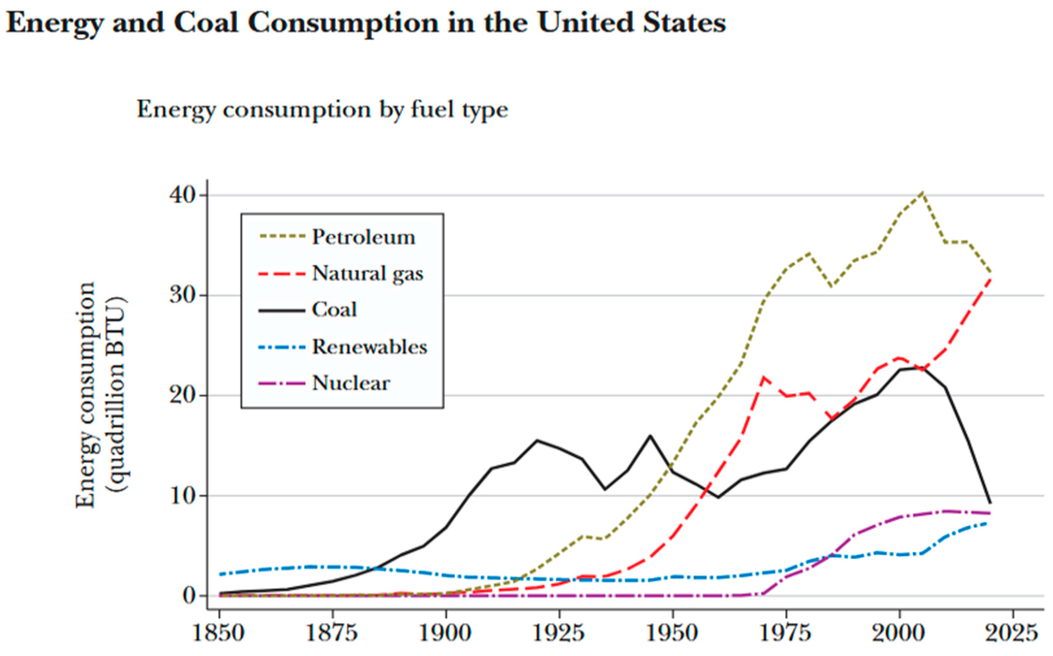
The trend in energy sources for the U.S. from 1850 to 2024 is shown in Figure 1 from Ref. [1]. Natural gas use has risen while coal and petroleum use have fallen in the past two decades, due mainly to electric generation fuel switching. Nuclear fission remains flat but is expected to rise as packaged nuclear generation plants, which should involve major reductions in financial, design and timing risk, are forthcoming. Some nuclear plants, closed because they could not compete on a price basis with natural gas plants, are expected to re-open due to (1) changing sentiments toward nuclear in the light of climate change, (2) the need to back up renewables generation, and (3) major forthcoming capacity needs due to AI data centers and increasing electrification (e.g., vehicles, space heating).

Since a small number of firms (less than 50 of them) in one industry produce the highest concentration of emissions in the U.S., this paper investigates the nature of the production function of CO₂ by U.S. utilities in the process of producing electric power. This research is one of very few papers that uses a production function to model a “bad” output in contrast to a good output.

The main methodological contribution of this paper is to model and empirically measure the efficiency of the U.S. electricity utility industry in reducing greenhouse gas emissions, or CO₂, and estimate the impacts of the contributions of generation technologies/fuel types on CO₂ emissions. Using a production function approach for estimation, considering CO₂ as the production output, a “bad” output rather than a good one, we find that nuclear, solar, wind, and hydropower reduce the total output of a utility’s CO₂ in the process of power generation and that gas provides a partial reduction relative to coal and oil. As a novel approach, power generation by fuel types are factor inputs and CO₂ the output. The summary result is that the U.S. utility industry has created diseconomies of scale in the production of the bad output CO₂. That is, if power generation is doubled, CO₂ output is less than doubled, demonstrating industry efficiency in reducing CO₂ emissions.

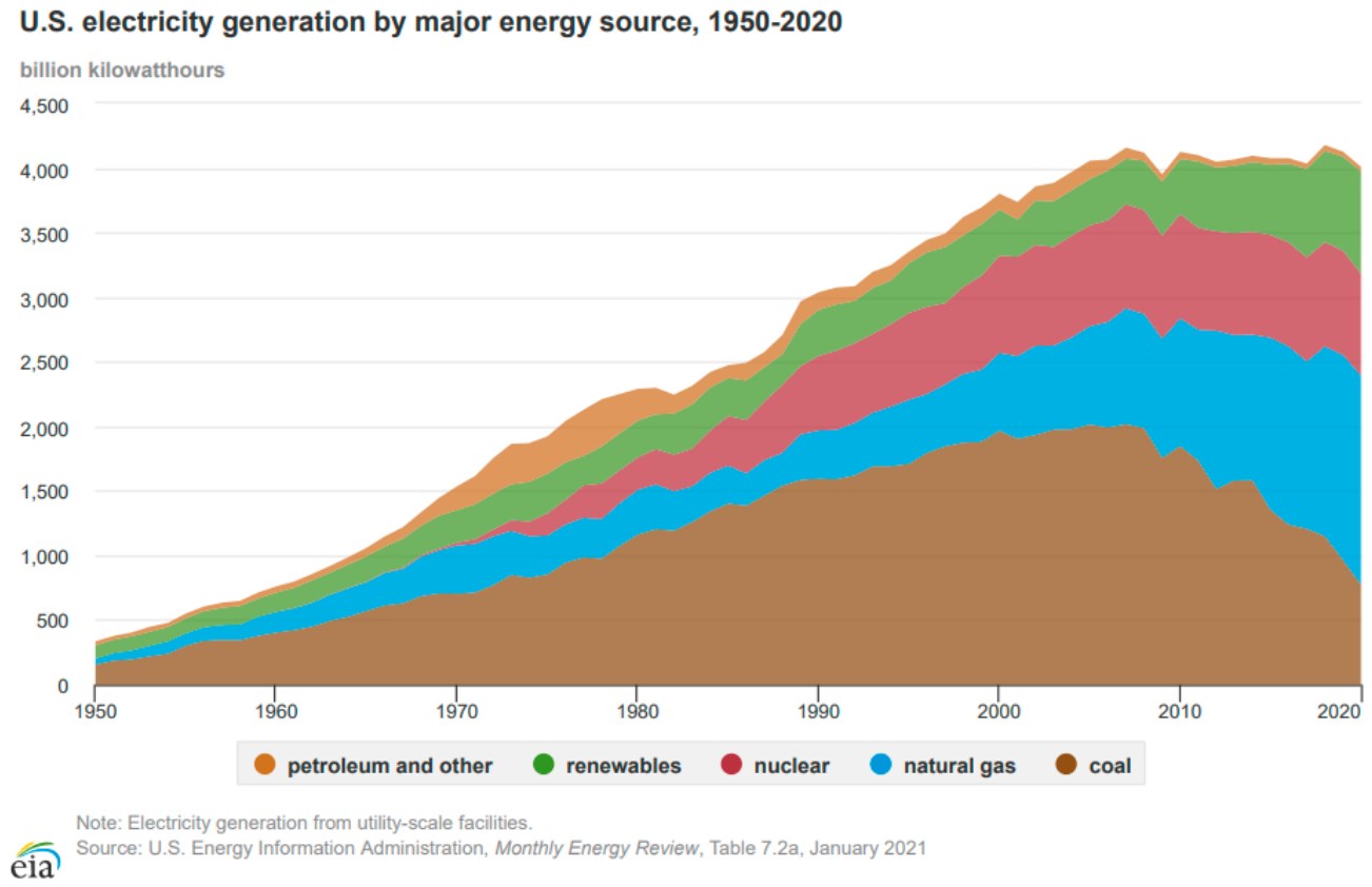
A review of the U.S. electric utility industry’s generation by fuel types for the last 70 years (1950–2020) is shown in Figure 2, a plot of GWHs (gigawatt-hours) generated by the U.S. electric utility industry by fuel type. The plot shows that, recently, the use of coal and oil is falling, natural gas is rising, nuclear is flat, and renewables (mainly wind and solar) are rising. Oil generation for base load generation is nil as utilities began substituting away from oil since the oil price and supply shocks in the 1970s. The diagram also shows that electric utility generation has been flat since the Great Recession that ended in 2009. That is mainly due to the adoption of efficient energy end-use technologies (such as high-efficiency household appliances, space cooling, electric motors, and LED lighting) and the accelerating diffusion of solar power projects owned by households, businesses, and other institutions. All these technologies reduce demand for utility power with efficient energy-using equipment and substitute usually clean self-generation, resulting in the reduction in the demand for utility power. The result is that U.S. utility power sales have been flat until very recently.

During the same time, utilities had been shifting away from coal and oil fossil fuels, not replacing their nuclear fleet of plants, and, at the margin, almost completely switching to wind and solar renewable generation. Note that there has been a substantial use of renewable power sources for many years, but historically they have been mainly hydropower plants. Also, nuclear power has recently been demonstrating a resurgence in the U.S. and Europe due to critically needed clean, large base–load power.

2. Literature Review and the Emissions Production Function

The literature clearly and consistently finds that electricity generation is a primary driver of global greenhouse gas emissions due to the combustion of fossil fuels [4] and a high positive correlation of energy consumption and emissions, sometimes at a level of 0.994 [5]. Recent studies (2025–2026) indicate a rising trend in low-carbon electricity generation globally, though progress is heterogeneous at the firm level [6,7]. In many regions, the rapid deployment of solar and wind technologies is directly displacing coal generation [6]. Approximately 40% of total global emissions originate from coal-fired power plants alone [8]. This is consistent with our modeling results below that show that, in the U.S., coal and oil power plants create the highest amount of CO₂ emissions for a given level of electricity generation. Ref. [9] examines the causal relationships between energy consumption, CO₂ emissions and GDP using a time-varying Granger causation approach for the G7 countries. They find that the time–variance relationship, among other relationships, between CO₂ and power production is from changes in country regulations, multinational agreements, use of pollution-abating technologies, natural disasters, economic cycles and composition of national economic sectors. Ref. [4] models the costs of CO₂ emissions from electricity generation in the U.S. and the benefits of co-pollutant reduction benefits (sulfur dioxide, nitrous oxide, and others) from CO₂ mitigation. This finding would result in higher potential economies of scale benefits from CO₂ by the industry, if the approach were to model all air pollution reduction from CO₂ mitigation.

A major contribution of this research is the classic production function approach for modeling economies of scale in reducing CO₂ as applied to one of the largest, if not the largest, single industry in the globe for creating CO₂ emissions: the U.S. electricity industry. We use a simple well-known and tested production function, the Cobb–Douglas production function. The purpose of this choice is to not distract from the core of the paper, which is the estimation of the efficiency in reducing CO₂ emissions in this industry and the relative contribution of fuel types and generation technologies in generating and reducing CO₂ emissions. The literature has provided a well-established analysis of the merits of the use and characteristics of various production function specifications, such as the constant elasticity of substation and the translog cost functions. The CO₂ and electricity generation and consumption literature adopt various forms and structures of customized regression models to estimate such relations. Although it is a simpler version of production function technology, we prefer to follow production theory to guide our research.

The form of production function used herein is the non-constant-returns-to-scale Cobb–Douglas production function (CD). The CD with n factor of production inputs is as follows:

$$Q=A X_1^{{\alpha }_1} X_2^{{\alpha }_2}{X}_3^{{\alpha }_3}{X}_4^{{\alpha }_4}\dots X_n^{{\alpha }_n}$$

(1)

where Q is the level of output, A is the total factor productivity parameter, X₁, …, X_n are the factors of production, and α₁, … α_n are factor of production elasticities of output. If α₁ + …+ α_n = 1.0, then the production function has constant returns-to-scale. Double the inputs X₁, …, X_n and the resulting output Q will double. If α₁ + … + α_n > 1.0, then there are increasing returns-to-scale. Double the inputs and output more than doubles and, for decreasing returns, ({α₁ + … + α_n} < 1.0), double the inputs, and output increases by less than double.

Another production function applied to model economies of scale and factor input substitution for electric utilities is the translog cost function. The advantage of the translog model is the flexibility in the substitution of the factor inputs across utilities. That modeling technology has not been adopted herein as it requires a lot of data that is largely not available, such as total costs for generation only. It also requires prices, total expenditures, and factor input shares for each factor input. It requires the estimation of the main equation and a series of equations, one for each factor input, simultaneously using the seemingly unrelated regressions method. For a standard application, it requires an additional three equations, one for each factor input, such as capital, labor and fuel. It requires many coefficient estimates (ranges from 10 to 20) that would overwhelm our small number of observations, especially as the specification requires log data. Our investigation is meant to be an early indicator of the efficiency for CO₂ mitigation by the single largest U.S. industry producer of CO₂ emissions that produces almost 1/3 of the CO₂ in the U.S., with lessons learned in the U.S. and implications for the world economy.

We are estimating the industry production function that uses all generation fuel types, not one for a specific utility, most of which do not use all generation fuel types. The intra-utility production function estimates may be subject to bias and inconsistency, but the industry production function should not be as it has all input types. The results are also consistent with a priori intuitive engineering coefficient estimates in both relative size and algebraic sign.

Rather than use the typical application of a production function to model the production of a good output, we use it to model a “bad” output, CO₂. We are particularly interested in the decreasing returns-to-scale case as we expect that as utilities have been using mitigating technologies to minimize emissions, decreasing returns should be realized in emissions production.

Refs. [9,10,11,12,13] specify emissions as driven by output in production functions and energy as a factor input. They develop computable general equilibrium models that perform simulations of energy efficiency investment and policy options that are meant to model pollution impacts because of production in the economy. Ref. [14] include sulfur dioxide (SO₂) emissions (that causes acid rain) as an input factor of production for electricity in a translog cost function (the cost function is the dual of production) specification. They find that substantial substitution occurs between SO₂ emissions, SO₂ permits to emit, capital, fuel, and labor and that SO₂ permit inventories are used to hedge SO₂ emissions risk. Ref. [15] specifies a multi-output production function: one is good (electric power) and one they refer to as bad, SO₂. They explain the shadow price of SO₂ emissions permits with their specifications and empirical analysis. Ref. [16] modeled emissions as a production input along with labor and capital with the Cobb–Douglas production function and found that the coefficient on the log of emissions is statistically significant at very low p values.

The less recent literature (before 2010) and U.S. EPA policy focused on nitrogen oxides, sulfuric oxides and particulates as these emissions directly affect human health and the environment (such as acid rain from SO₂). With the recent focus on climate change and greenhouse gas emissions, the attention has turned mainly to CO₂. However, the recent and older literature both provide guidance on modeling CO₂ emissions from electricity production.

This investigation estimates a production function to quantify economies of scale, the MRTSs (marginal rates of technical substitutions) between generation fuel types (inputs) as electric utilities, and other generation plant owners who mitigate emissions output by substituting fuel types. (Most retired coal plants were replaced by natural gas and, to a much lesser extent, renewables.) Electricity generation can be viewed as the same as energy consumed except for line losses. Supply is instantaneously demand-driven and cannot be cost-effectively stored in bulk.

In the specification and estimation of the emissions production function, we place no a priori returns-to-scale restrictions on the production function. It is hypothesized that the emissions production function has decreasing returns to scale as producers of electricity strive to mitigate emissions output as they meet the demand for power.

Like Ref. [13] we specify emissions as the output of a production function driven by factor inputs. Refs. [17,18] specify emissions as an input to produce, and, as a function of energy produced, respectively. We specify factor inputs as the volumes of electric power generated by the major fuel types used by electric utilities and other power generators: from fossil fuels (natural gas, coal, and oil), nuclear fission, and renewables, solar, wind and hydropower. One could view electricity output as a surrogate for the capital, labor and other factors of production used to produce electricity. We separate natural gas from oil and coal as natural gas produces substantially less emissions per megawatt-hour (MWH) output than the other fossil fuels and is almost 50% more efficient than coal combustion. The average efficiencies are 33% for coal and 46% for natural gas. (Most retired coal plants were replaced by natural gas and, to a much lesser extent, renewables.) The remainder of the heat produced in the process (100%—efficiency %) goes up the plant stack into the atmosphere, except for co-generation plants that capture what would be waste heat and convert it into steam that is sold to a steam host customer (usually large institutional and industrial facilities). The key difference between the fuel types’ engineering efficiency is indicated by the energy conversion ratio, or “heat rate” in industry parlance, which is the ratio of the British Thermal Units (BTUs) of fuel input required to produce 1 kilowatt-hour, KWH or BTU/KWH. The heat rate is theoretically similar within the same fuel type but very different across fuel types. Efficiency is the reciprocal of the energy conversion factor. (With perfect efficiency in energy conversion, 1 KWH is equivalent to 3412 BTUs, so it would take 3412 BTUs of fuel input with perfect efficiency to generate 1 KWH. The typical base coal plant in the U.S. runs at about 33% efficiency, which means that it takes 10,339 BTUs of input coal to generate 3412 BTUs of electric output, 1 KWH (efficiency = 1/heat rate = 1/{10,339/3412} = 0.33). Combined cycle natural gas plants have a typical heat rate of 7340 BTUs per KWH or are 46% efficient (.46 = 1/{7340/3412}). Heat rate data from the U.S. EIA’s Form EIA-860. Data Tables are available upon request.) They are complex to quantify for some fuel types, such as hydroelectric, nuclear, wind and solar power, but are important as these systems create no direct carbon emissions in the production of electricity. A standard approach would use BTU input as a factor of production, so the use of KWHs generated reflects different conversion ratios of the BTUs to KWHs. Here, we use gigawatt-hours (GWHs) volumes produced as inputs. A pure theoretical engineering approach would be to use conversion rates among fossil fuel types for differences in emissions and 0 for nuclear and renewable energy fuel types. We do not use theoretical engineering conversion rates as the actual operating emissions data from plant use are far different than theoretical physical estimates. (Theoretical engineering conversion rates are useful for plant design and developing general estimates of the carbon emissions by fuel type. They also serve as a general guideline for what is possible to expect from actual plant data. But the operating data can be far different than theoretical engineering conversion rates. If all plants in the utility portfolio are not all running at capacity, the actual emissions can deviate substantially from the conversion rates. For example, if the utility uses nuclear and natural gas only and the nuclear plant has a forced outage or is being re-fueled with new fuel rods, either of these will result in the plant being offline for months. Since natural gas is the sole power-producing plant type and the utility has enough gas plant reserve, all of the power is produced by natural gas. There are many combinations of plant types that may or may not be operating relative to the portfolio of plant types owned by the utility. There are also differences between new and older-technology plants (e.g., single-cycle v. combined-cycle natural gas plants). Combined-cycle plants capture and use the otherwise waste heat from the initial gas turbine to power a secondary steam turbine, significantly increasing the total electricity generated from the same amount of fuel and emissions, and are 50 to 60% more efficient than single-cycle plants. There may be co-generation plants, usually fired by natural gas, that also use the otherwise waste heat byproduct. Fuel quality, the quality of plant maintenance practices, and many other variables can also substantially affect the actual v. theoretical conversion rates and therefore affect the production efficiency of CO₂ emissions. The relative contribution of the actual emissions reductions by “fuel” types for actual output generation of power is not known without regression. This involves a substitution question, and production functions are naturally suited to address such questions. However, it is not the only approach to address substitutions, such as that presented in the work of Ref. [19].)

The unrestricted (no a prior specification on returns to scale) production function is

$$Q_{i,t}={\alpha }_0 F_{i,t}^{{\alpha }_1} G_{i,t}^{{\alpha }_2} H_{i,t}^{{\alpha }_3} N_{i,t}^{{\alpha }_4} R_{i,t}^{{\alpha }_5} e^{{\epsilon }_{i,t}}$$

(2)

where Q_i,t is the output of CO₂ emissions by firm i at time t; F_i,t, G_i,t, H_i,t, N_i,t, and R_i,t are, respectively, the power volumes generated by fossil fuels other than natural gas (coal and oil), natural gas, hydropower (water power), nuclear fission, and renewable energy (solar and wind) for firm i at time t. Hydropower is also a form of renewable energy. These can also be viewed as the electricity used by fuel type in the production of emissions.

The α_is except for α₀ are the emissions output elasticities of each fuel type, and α₀ is the coefficient of total factor productivity. The term ε_i,t is the regression error term. We hypothesize that α₁, the coefficient for oil and coal generation, and α₂, the natural gas emissions output elasticity, are positive. But the natural gas coefficient should be materially less than other fossil fuels as it combusts much more efficiently and generates less emissions. The slopes α₃, α₄, and α₅, for hydropower, nuclear and renewable generation, respectively, are negative as coal and oil are the least energy efficient as they generate the highest level of emissions for a given level of output and the others generate power with no emissions output. As the utility switches to non-fossil fuels to generate power, the emissions output will decline further.

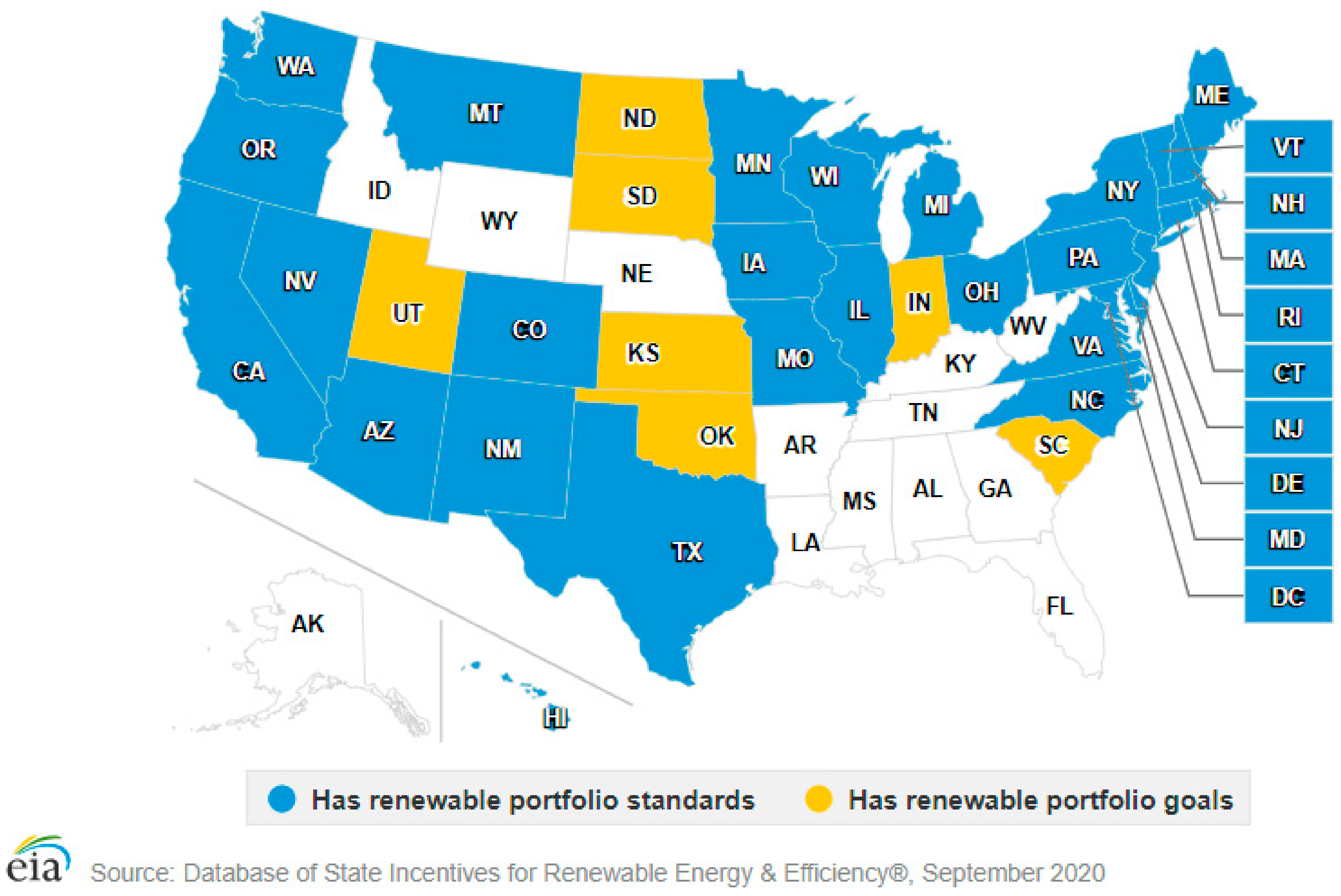
Since electric utility firms are subject to the Clean Air Act II, and many states have renewable portfolio requirements for electric utilities that are required to sell increasingly greater shares of power produced from renewable energy (as shown in Figure 3), electric utilities have been decommissioning coal plants, investing in and buying more power from combined-cycle (more efficient than single-cycle) natural gas plants and renewable projects, and have enacted very limited re-commissioning of nuclear plants for longer service lives. Only two new nuclear units (one project with two units) have recently been developed in the U.S. at the time of writing this paper. They are the two Vogtle reactors with a capacity of 1117 MWs each, located near Augusta, Georgia, and mainly owned by Southern Company. The budget has risen from an initial $14 billion to $28 billion; the units were to be operational by 2017 and are now operating as of 2024. This déjà vu adverse experience of nuclear plant development from the 1980s makes it unlikely that additional large base load nuclear plants will be newly built in the U.S. However, there are many that are being refurbished or filing for permission to extend the life of older units. Smaller modular reactors are in development experimental modes currently. They are approximately 500 MWs in size. There is one under construction in Tuckerton, New Jersey, at the Oyster Creek Nuclear Power Plant Site where the former large base load plant was closed due to the cost of upgrading the cooling system. The cooling system was causing thermal pollution (increasing the temperature) in the waters of the Barnegat Bay, and a cooling tower investment was made a requirement of its re-licensing, so it was closed by the owners at the time as it was not cost-effective to its investors.

An important empirical question concerns the MRTS among fuel inputs between those that do and do not generate emissions experienced by the industry. (There has been major substitution between coal and natural gas in the past 10 years or so. There has been very little oil use in recent decades, except for its use for combustion turbines that are only used a few hours per year during peak load days. They are jet engines fired by kerosene with inexpensive capacity costs that are easy to install but have high variable costs. The trend in oil being pulled from base load generation fuel mix started after the two oil price and supply shocks in the 1970s. We develop the heat rate conversion factor between natural gas and coal above, and the conversion rate for CO₂ emissions is similar. The heat rates are substantially different between coal and natural gas. So, a matter of perspective is whether natural gas is a pseudo-clean resource regarding CO₂ emissions reductions relative to coal. Also, utilities in many states are subject to renewable portfolio standards, which means that they must use by law and deliver the specified percentage of their output from renewable energy. They must purchase renewable energy credits from the owners of the renewable energy plants or their output. So, in effect, they do make substantial substitutions from fossil fuels to renewable energy. See Figure 3 and the associated discussion. Most states have a portfolio renewable standard, many of which are mandates baked into state laws. Many of them require major mixes of renewables in the range of 20 to 40% of all power sold in the near term and much higher in the long term. For example, the State of New Jersey (NJ) mandated that 35% of all power sold in NJ come from renewable energy as of 2025 and 80% by 2050.) Although we use the production function approach to model fuel-type substitutions in addition to economies of scale, both of which the production function literature was developed for, it is not the only approach to model fuel-type substitutions. Ref. [19] performed regression modeling analysis of direct fuel displacement of coal and oil by natural gas, nuclear, hydro, and renewable energy for 40 countries. The results show that substitution is small for nuclear, relatively larger for natural gas and hydro, and solar and wind have the largest substitution impact. We would expect that nuclear power will grow in impact as it has very recently received renewed focus. That is because it is the only large-scale, base load power plant type that has no CO₂ emissions. Renewables are trending into a larger role, but they require backup generation as they are mainly dispatched by weather.

MRTS is the rate at which one input factor can be substituted for another without changing the level of output. It can also be shown that it is the ratio of the marginal products of two factors of production. Given a generic production function with two factor inputs labor (L) and capital (K), Q = f (L,K), take the total differential and set it equal to 0 as we seek the needed substitution level between K and L to keep Q constant (subscripts refer to partial derivatives with respect to Q): dQ = f_L dL + f_K dK = 0. Solving for MRTS, which is the change in one factor relative to the other factor input, we get −dK/dL = f_L/f_K. That is, MRTS_L,K = MP_L/MP_K. MP_L, for example, refers to the marginal production increment of output generated by increasing labor one unit (one hour,…). For example, MRTS_F,R = −dF/dR = MP_R/MP_F. The MPs of emissions for non-fossil fuels are negative. As you generate more power with non-fossil fuels, you increasingly substitute the use of fossil fuels and emissions fall. Therefore, the MRTSs between non-fossil fuels and fossil fuels should be negative if the utilities are aggressively substituting non-fossil fuels for fossil fuels.

To estimate the MRTSs, we estimate the natural log form of Equation (1). Lowercase letters refer to the log of each variable:

$$q_{i,t}={\alpha }_0+{\alpha }_1{f}_{i,t}+{\alpha }_2{g}_{i,t}+{\alpha }_3{h}_{i,t}+{\alpha }_4{n}_{i,t}+{\alpha }_5{r}_{i,t}+{\epsilon }_{i,t}$$

(3)

The MRTSs among the various fuel types and fossil fuels are as follows (subscripts refer to partial derivatives). The first one below in Equation (4) is the example of the MRTS between renewables and fossil fuels excluding natural gas:

Renewable:

$$Q_{r,f}={\displaystyle \frac{\partial r}{\partial f}}={\displaystyle \frac{1}{\frac{\partial q}{\partial r}}}{\displaystyle \frac{\partial q}{\partial f}}={\displaystyle \frac{{\alpha }_1}{{\alpha }_5}}$$

(4)

Therefore, the other MRTSs with fossil fuels except natural gas are the following:

Natural Gas:

$$Q_{g,f}={\displaystyle \frac{{\alpha }_1}{{\alpha }_2}}$$

(5)

Hydropower:

$$Q_{h,f}={\displaystyle \frac{{\alpha }_1}{{\alpha }_3}}$$

(6)

Nuclear:

$$Q_{n,f}={\displaystyle \frac{{\alpha }_1}{{\alpha }_4}}$$

(7)

The parameters α₃, α₄, and α₅ are hypothesized to be negative as their increased use as a substitute for fossil generation will cause emissions output to decline. Their MRTSs are negative. This is an adverse result if producing a good output, as far too much substitution in the U.S., of a factor input is occurring to the point that the marginal product from the factor input is negative. This is analogous to substituting so much labor for capital that congestion is occurring at the production site, and resulting additional output from adding more labor to too little capital is declining. For the production of a “bad” output, this is a favorable outcome. R is so intensely substituted for F that the MP_R is negative. The MRTS estimates show the experienced redemption as they strive to reduce CO₂ greenhouse emissions by fuel substitution to clean inputs. The natural gas MRTS (Q_g,f) shows the level of switching reduction in the growth of emissions when switching from coal/oil to natural gas to maintain a constant level of emissions. The other coefficients quantify the reduction in emissions from fuel switching away from non-gas fossil fuels. The factor MRTSs with negative signs are interpreted as follows. As you reduce the use of factor input, say, coal (percentage change in the generation of GWHs from coal falls), you increase the percentage change in another factor (you increase the percentage change in generation of GWHs from renewables).

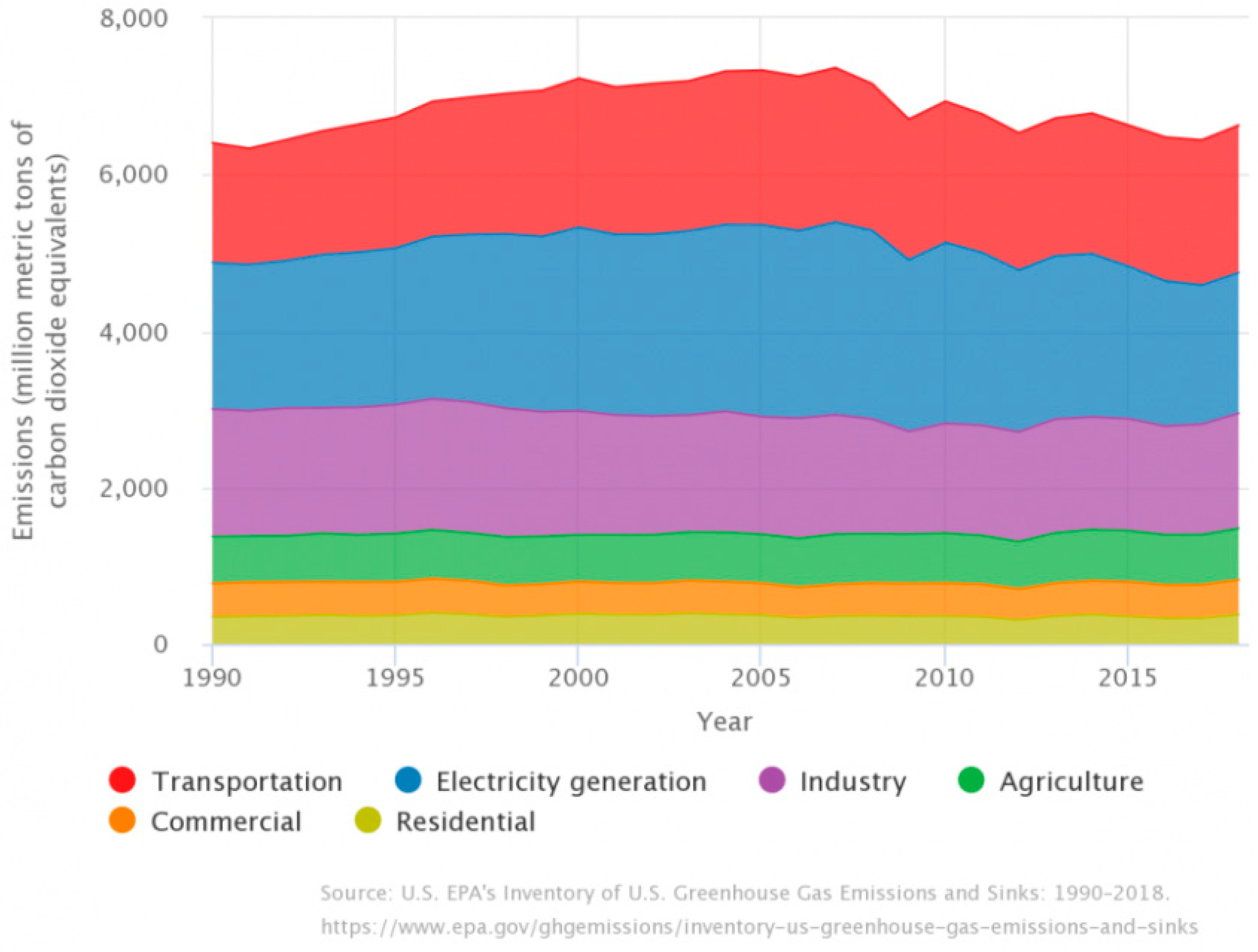
Another important issue is whether the electric utility industry has increasing, constant or decreasing returns to scale in the production of CO₂ emissions. Figure 4 shows that emissions from the entire electricity utility sector of the economy are dropping while power production has changed from flat to slightly growing, which is an intuitive indicator of decreasing returns to scale. It also shows that electricity generation is the largest CO₂ emitter of all the key economic sectors in the U.S. It is moderately higher than transportation.

If all the factor input parameters sum to 1 {(α₁ + α₂ + α₃ + α₄ + α₅ = 1)}, there are constant returns to scale in emissions production. If they sum to more (or less) than 1, there are increasing (decreasing) returns to scale. Since we are modeling a production function for a “bad” output, it is desired to have decreasing returns to scale. That is, as we grow electricity production over time or as electricity production remains flat, emissions output should drop.

3. Data and Empirical Results

Our emissions and power generation data are from Bloomberg Finance L.P. The original source of most of the emissions data that we extract from Bloomberg is the CDP (formerly the Carbon Disclosure Project). The CDP is an international non-profit organization that requests information from the world’s largest companies on behalf of institutional investors. Recently, the CDP had over 590 institutional investor signatories with a combined $110 trillion in assets. Each year since 2003, the CDP has distributed questionnaires encouraging corporations to disclose annual CO₂ emissions and other climate-related information in a standardized way. Any corporation’s decision to disclose is voluntary. In our sample, Bloomberg occasionally supplements CDP data with emissions reported in publicly available corporate sustainability reports.

Our emissions data are Scope 1 emissions, which are direct GHG emissions from facilities controlled by a company and under their control, such as emissions from fossil fuels used in production. GHGs are those that contribute to the trapping of heat in Earth’s atmosphere, including CO₂, methane, and nitrous oxide. Emissions of gases other than CO₂ are converted to CO₂ to produce an overall measure of firms’ GHG emissions. Scope 1 emissions are by far the predominant source of emissions for producers of electricity in the U.S. We expect Scope 1 emissions to be accurately measured by power producers, because power producers have been required by the U.S. EPA to measure and report direct emissions hourly by generating facility location since 1995. For consistency of measurement and to maximize our sample size, we exclude Scope 2 and Scope 3 emissions, both of which are small relative to Scope 1 emissions for our sample firms and less often disclosed. We extracted 290 Scope 1 and 222 Scope 2 firm-year observations from Bloomberg. Mean Scope 1 and Scope 2 emissions are 32.8 million and 1.7 million metric tons, respectively. Moreover, there has been less consistency in the methods used to measure Scope 2 and Scope 3 emissions. Scope 2 emissions are indirect, coming from the generation of purchased heat, steam, and electricity purchased and consumed by a company. The methodology for reporting Scope 2 emissions to CDP changed in 2015. Scope 3 emissions are the result of activities from assets not owned or controlled by the reporting company but that the company indirectly impacts in its value chain. There is less agreement as to how to accurately measure Scope 3 emissions, so Scope 1 and Scope 2 emissions are more consistently reported by data providers than Scope 3 emissions.

Our Bloomberg sample of 48 investor-owned U.S. power producers consists of 28 electric utilities, 15 multi-utilities, and 5 independent power producers. Thirty-four Scope 1 emissions were reported during the years 2006 to 2018. The available data is sparse as utilities consistently began reporting greenhouse emissions voluntarily in 2006 on a total utility basis. Our data sourced from Bloomberg consists mainly of CDP data but is supplemented in a few cases by utilities’ sustainability reports. The CDP is an organization in the United Kingdom, Japan, India, China, Germany and the United States. The CDP has been reporting voluntary disclosures by companies and governments of their environmental impacts since its inception in 2002. Over 8400 companies to date publicly disclosed environmental information through the CDP. GWHs generated by fuel type for each utility are obtained from the Bloomberg data system.

Since utilities produce or buy power from different generation portfolios, many do not have nuclear, hydropower, or renewables produced power. Also, some do not have coal or oil, although most do have natural gas. There are 48 firms in our investor-owned utility universe and a potential of 13 years of emissions data from 2006 to 2018 (data is incomplete for some utilities) which therefore includes time series and panel observations. Of the universe of utilities, 33 reported CO₂ emissions and had emissions data and 15 did not. Therefore, a potential of 34 utilities with a maximum of 13 years of time series are included in the regressions. Due to missing years of emissions data and some utilities not having all fuel types (many do not have nuclear or hydropower), this reduces the total dataset for the regressions when using logs to estimate the model.

The emissions data are metric tons of CO₂ directly produced by the generation assets of the specific firm (Scope 1). The other two CO₂ emissions variables are as follows: Scope 2 emissions come from the generation of purchased heat, steam, and electricity consumed by the company. Scope 3 emissions are caused by supply chain impacts on emissions and occur from sources not owned or controlled by the company. These include emissions from the production of purchased materials, product use, waste disposal, and outsourced activities. We address Scope 1 emissions only.

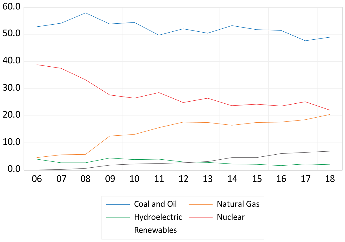
Figure 5 shows the trends in the percentage of each fuel type used by the electric utilities in the sample. Whereas coal and oil are in long-term decline, natural gas and renewable energy have risen. Nuclear generation is also in long-term decline. As utilities retire old plants, they do not want the exposure of the investment risk associated with building new nuclear generation and the physical and financial risk of operating them, regardless of the recent resurgence in the acceptability of nuclear power.

Figure 6 lists all the investor-owned electric and electric and gas utilities in the data set. Only a few of them have all fuel types. Therefore, to maximize the number of retained observations, we combine hydro and renewables as an alternative variable, as both are renewable and do not produce emissions, and coal/oil and natural gas as one variable in an alternative regression model (Model 2). Renewables were historically defined in the industry as those energy sources that have an inexhaustible supply, but some of them produce emissions such as methane gas from landfills that are used to fuel a power plant. The original intent of identifying resources as “renewable” was to secure inexhaustible energy supply sources as we reached the exhaustion of finite energy resources [22]. Others are spent vehicle tires, wood, other biomass, corn ethanol and other organic fuels that can be burned in a power plant combustion chamber. They are not included in the definition of renewables for this research as the recent definition includes only those that are environmentally sustainable and produce no CO₂ emissions or other GHG emissions.

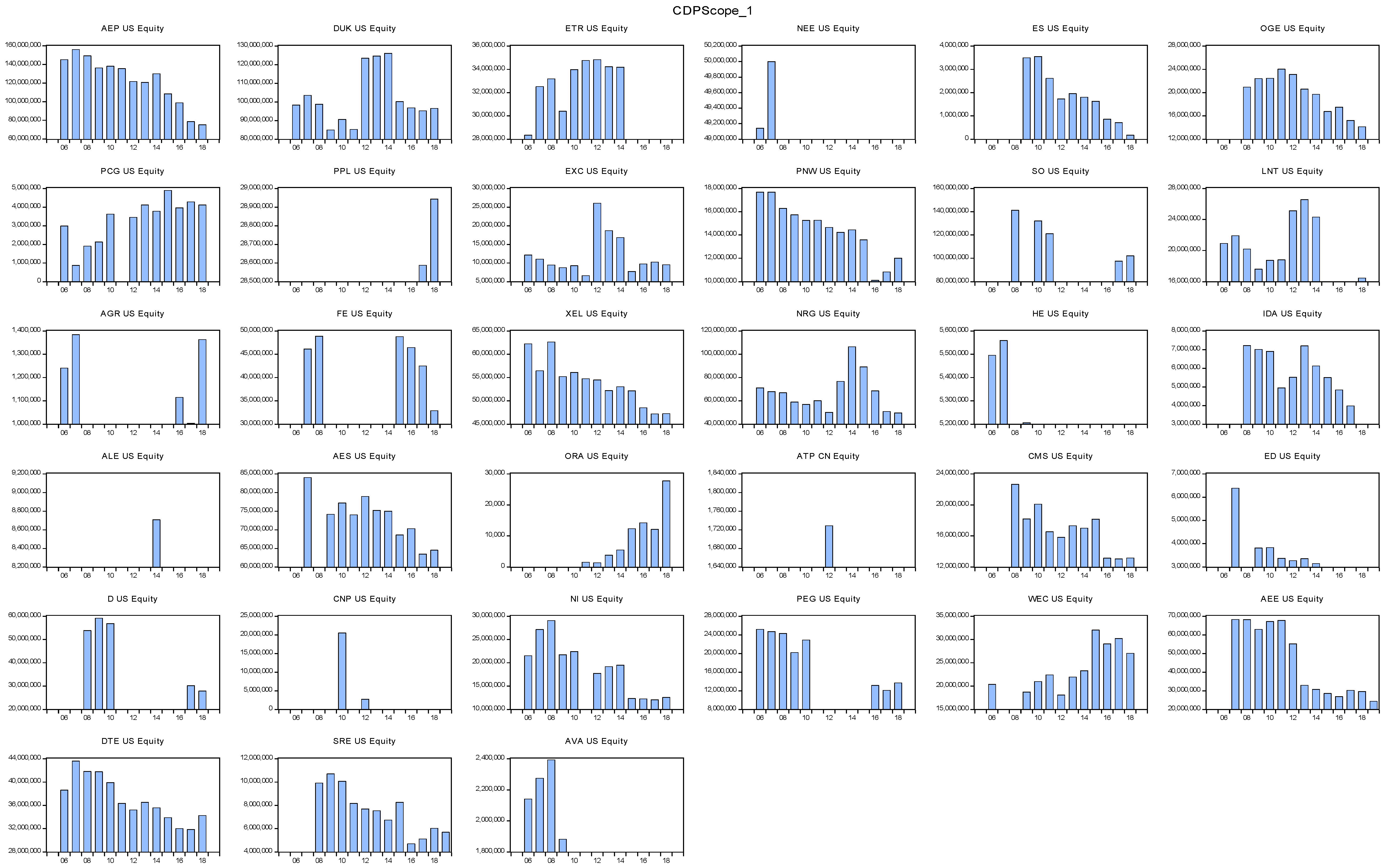
Figure 7 shows the CO₂ trend for every utility in the dataset from 2006 to 2018. Data is incomplete for many utilities. The data shows a general downward trend in emissions for most utilities. It also shows the extent of the missing data and sparseness in the dataset.

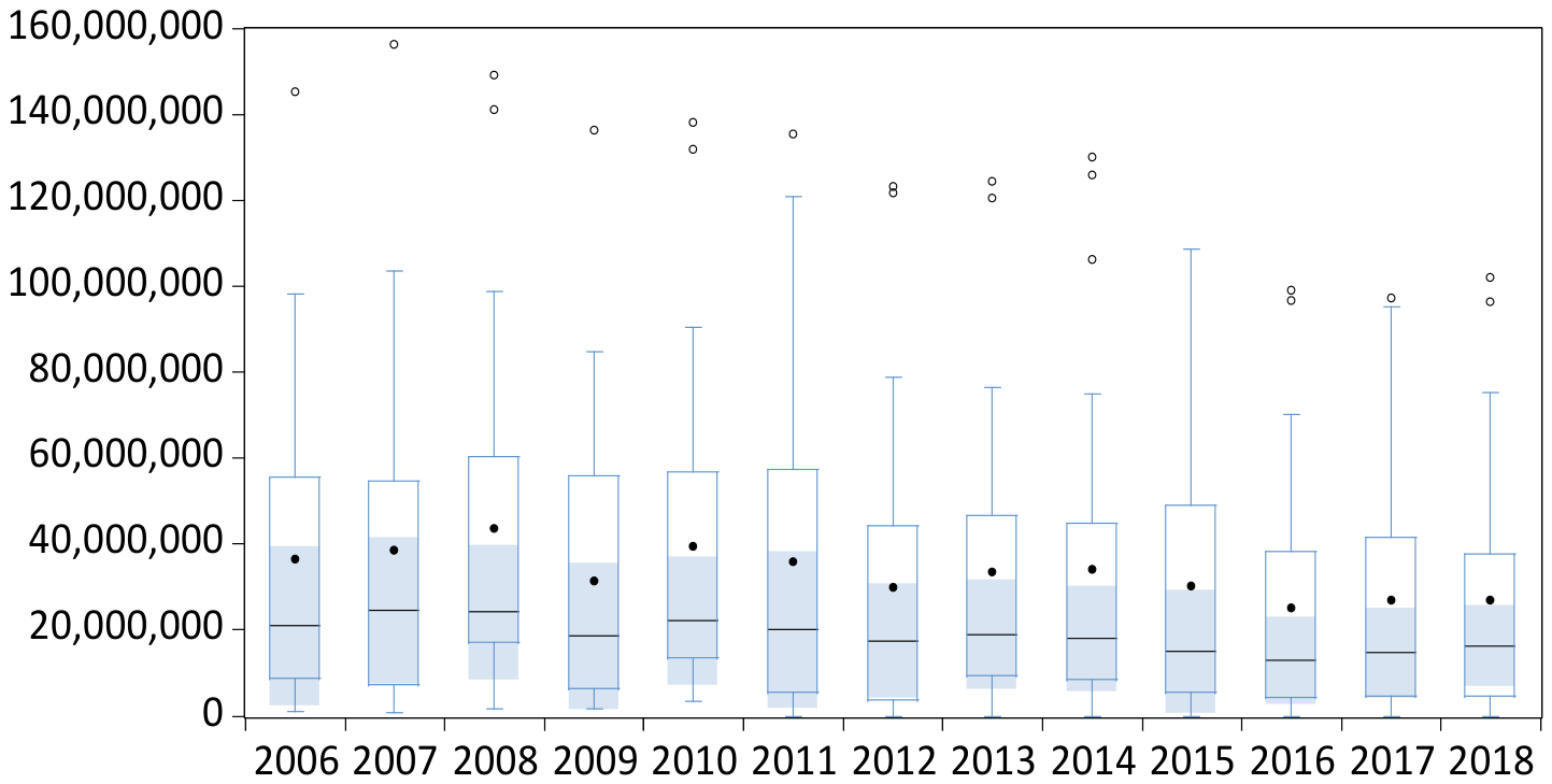
The data includes the Scope 1 CO₂ emissions in metric tons voluntarily reported to the Carbon Disclosure Project by each utility in the dataset for which there is data from 2006 to 2018. As can be viewed above, data is incomplete and reporting is aberrant for some utilities. Figure 8 shows the boxplots of the CO₂ emissions for the industry for the years 2006 to 2018. A review of boxplots is analogous to looking down at the distributions of the data for each period. The plots are non-parametric distributions. The boxplots show the 25th and 75th percentiles (the box height), the 10th and 90th percentiles (the whiskers), the median (the line inside the box), and the dispersion of the emissions. They also provide the mean, the minimum and maximum values. Dots represent the means of the data. The boxplots indicate that the data is highly skewed as the median of the data of all utilities for every year but 2018 is substantially lower than the mean. This indicates that the emissions output is concentrated within a few utilities. All outliers are above the upper whisker and therefore very large, and there are no outliers that are very low. Both medians and means of emissions are on a slowly declining trend, although emissions for some interim years have increased. That can still occur even with aggressive mitigation. Power demands and generation levels are determined by the strength of the economy as well as the extremity of weather in summer and winter that drives power needs for space cooling and heating. Therefore, they drive the usage of fossil fuel plants.

Prior to estimating the production function, raw emissions data are regressed on the GWHs production data for each fuel type to view the relation between generation levels and emissions. Coal and oil are power generated by fossil fuels other than natural gas. Gas is power generated by natural gas. Hydro is hydroelectric power generation other than pumped hydro which is included in renewable. Nuclear is nuclear power generation. Renewable is all generation from clean renewable sources. CO₂ is the carbon dioxide equivalent of emissions in metric tons. The sample consists of all years in which emissions were reported during the period 2006 to 2018 and for which the sources of power generation are available on Bloomberg.

Voluntary disclosure can potentially introduce self-selection bias when the data is reported. If missing data shows adverse results, that can cause the results to be biased as better than actual. Missing data can affect coefficient stability and interpretation, but our results as presented below are consistent with engineering intuition. Emissions data are publicly disclosed to the U.S. EPA by law, so it is not likely that only positive data is reported. The U.S. EPA has required continuous monitoring (hourly metering) of CO₂ as well as other emissions such as nitrous oxide, sulfur oxide and particulates from fossil fueled power plants greater than 25 MW in capacity since 1 January 1996. Therefore, the utilities had detailed metered data on CO₂ from their plants before our time period of observation starting in 2006 from Bloomberg, well after the CPD voluntary disclosure started. The challenge with using such granular (hourly) data is mapping the trail of the owners’ thousands of plants and assigning them to a specific utility, which is a monumental undertaking and, as far as we are aware, has not been done yet. We are not sure why utilities did not report voluntarily when they had such granular data on emissions, but we were limited by the data that is available.

Missing data for explanatory variables occurred as not every utility has all plant fuel types for generating power. Such data were assigned 0s. Many utilities do not have all these types of plants for generation in our analysis: coal/oil, natural gas, nuclear, wind, solar and hydropower.

The estimation results are shown in

Table 1. Regression of Scope 1 CO₂ emissions on generation output by fuel types.

Variable	CO2/1000
Coal & Oil	0.910 (0.011) ***
Gas	0.571 (0.025) ***
Nuclear	−0.041 (0.012) ***
Hydro	−0.206 (0.099) **
Renewable	−0.343 (0.069) ***
Constant	2251.58 (2.32) **
R-square	0.98
No. of Obs.	216

The coal and oil variable is power generated (GWHs) by fossil fuels other than natural gas. Gas is power generated by natural gas. Hydro is hydroelectric power generation other than pumped hydro which is included in renewable. Nuclear is nuclear power generation. Renewable is all generation from renewable sources. CO₂ is the carbon dioxide equivalent of emissions in metric tons. The sample consists of all years in which emissions were reported during the period 2006 to 2018 and for which the sources of power generation are available on Bloomberg. **, *** refer to p values for statistical significance at 0.05. and 0.01 levels using a t-test.

. The results are robust as the r-squares are very high and all coefficients for fuel-type generation are significant at either p = 0.01 or 0.05. As expected, the coefficients are positive for the fossil fuel variables coal and oil, and natural gas, as they generate emissions, and negative for the non-fossil fuel variables. Additionally, the slope on natural gas is about 50% less than coal and oil as coal and oil combustion are less efficient than natural gas at 46% versus 33% (see footnote 1). Nuclear, hydropower, and renewables emit no CO₂, and their slopes are all negative as they generate electric power with no emissions output. These results are evidence of the credibility of the emissions and generation data.

Next, the production function is estimated. The regression results of Equation (3), noted as Model 1 in

Table 2. Production function regressions estimations.

	Model 1  $\begin{array}{c}{q}_{i,t}={\alpha }_0+{\alpha }_1{f}_{i,t}+{\alpha }_2{g}_{i,t}+{\alpha }_3{h}_{i,t}+{\alpha }_4{n}_{i,t}\\ +{\alpha }_5{r}_{i,t}+{\epsilon }_{i,t}\end{array}$		Model 2  $\begin{array}{r}{q}_{i,t}={\alpha }_0+{\alpha }_1{\log (F}_{i,t}+G_{i,t})+{\alpha }_2\log \left(N_{i,t}\right)\\ +{\alpha }_3\log \left(R_{i,t}+H_{i,t}\right)+{\mu }_{i.t}\end{array}$
	Coefficient	Standard Error	Coefficient	Standard Error
Fossil without Gas (fi.t)	0.419 ***	0.040
Fossil Fuels with (Fi.t + Gi.t)			0.900 ***	0.030
Gas (gi.t)	0.388 ***	0.063
Hydro (hi.t)	−0.022	0.049
Nuclear (ni.t)	−0.161 ***	0.054	−0.265 ***	0.043
Renewables (ri.t)	−0.050	0.047
Renewables and Hydro (Ri.t + Hi.t)			−0.081 ***	0.023
R-Square	0.96		0.91
No. of. Obs.	33		94

Model 1 and Model 2 were estimated using panel least squares. The data includes Scope 1 greenhouse emissions CO₂ in metric tons as the dependent variable and electric power generated by fuel type in MWHs as the independent variable. The annual data is for 33 electric and electric/gas utilities for the period 2006 to 2018. Data for all years is incomplete for some utilities. All data is converted into natural logs as denoted by the lowercase letters in Equation (3). *** denotes statistical significance at the p value of 0.000 in a two-tail t test.

, include all fuel types as separate input variables and show that all non-fossil fuels parameter estimates are negative. They should be negative as they produce no emissions as GWH volumes grow. The fossil fuel coefficients are positive as they generate emissions with growing GWHs. The fuel-type coefficients sum to less than one, which indicates decreasing returns to scale. One issue is that as the log transformations of the variables are performed, we lose much of the data as many utilities do not have all fuel types and therefore have zero values, which causes observations to be dropped as zeros cannot be log transformed to a discrete finite value (the natural log of zero is negative infinity: lim e^x = 0 as x → −∞). Comparing the first raw data regression to the production function regression, the number of observations drops from 216 to 33. (We considered the use of replacing 0s with a very small positive number such as 0.0000001 so that when converting to logs, the resulting values would be very close to zero and preserve more observations, but that would be a misspecification of the data and model; we did not use that approach. We did estimate it and it yielded no tractable results.)

The second regression (this model adds other fossil fuels and natural gas as one variable and renewables and hydropower as individual variable as follows: $q_{i,t}={\alpha }_0+{\alpha }_1{\log (F}_{i,t}+G_{i,t})+{\alpha }_2\log \left(N_{i,t}\right)+{\alpha }_3\log \left(R_{i,t}+H_{i,t}\right)+{\mu }_{i.t}$ (“Model 2”) estimation results shown in Table 1 combine renewables and hydropower, as both are renewables, and all fossil fuels (coal, oil and natural gas), respectively, as single variables. This increases the number of observations from 33 to 94. The non-fossil parameter estimates, nuclear and renewables plus hydropower, are negative and the fossil fuel parameter is positive. All slopes are significant at p = 0.001, and the r-square is 0.91.

As shown in

Table 3. Factor input MRTSs and economies of scale estimates. Panel 1: Model 1: $q_{i,t}={\alpha }_0+{\alpha }_1{f}_{i,t}+{\alpha }_2{g}_{i,t}+{\alpha }_3{h}_{i,t}+{\alpha }_4{n}_{i,t}+{\alpha }_5{r}_{i,t}+{\epsilon }_{i,t}$.

	α1	a2	α3	α4	α5	α1 + … + α5 Economies of Scale
Estimate	0.419	0.388	−0.161	−0.022	−0.053	0.571
Wald Statistic α1 + … + α5 = 1						338.83 (p = 0.0000)
$Q_{r,f}={\displaystyle \frac{{\alpha }_1}{{\alpha }_5}}$	−7.906
$Q_{g,f}={\displaystyle \frac{{\alpha }_1}{{\alpha }_2}}$	1.080
$Q_{h,f}={\displaystyle \frac{{\alpha }_1}{{\alpha }_3}}$	−2.602
$Q_{n,f}={\displaystyle \frac{{\alpha }_1}{{\alpha }_4}}$	−19.045

The factor marginal rates of technical substitution (MRTS) among the various fuel types and fossil fuels are as follows (subscripts refer to partial derivatives). As an example, the MRTS between renewables and fossil fuels excluding natural gas is $Q_{r,f}={\displaystyle \frac{\partial r}{\partial f}}={\displaystyle \frac{1}{\frac{\partial q}{\partial r}}}{\displaystyle \frac{\partial q}{\partial f}}={\displaystyle \frac{{\alpha }_1}{{\alpha }_5}}$. The coefficients were estimated with Model 1 (Equation (3)) using panel least squares. The data includes Scope 1 greenhouse emissions CO₂ in metric tons as the dependent variable and electric power generated by fuel type as the independent variable in MWHs. The annual data is for 33 electric and electric/gas utilities for the period 2006 to 2018. Data for all years is incomplete for some utilities. All variables are converted into natural logs as denoted by the lowercase letters in Model 1. The Wald Statistic tests the null hypothesis that the sum of coefficients is equal to 1.0 which infers constant returns to scale. It is both F and chi-squared distributed as these values are the same.

and

Table 4. Panel 2. Model 2: $q_{i,t}={\alpha }_0+{\alpha }_1{\log (F}_{i,t}+G_{i,t})+{\alpha }_2\log \left(N_{i,t}\right)+{\alpha }_3\log \left(R_{i,t}+H_{i,t}\right)+{\mu }_{i.t}$.

	α1	α2	α3	α1 + α2 + α3 Economies of Scale
Estimate	0.900	−0.265	−0.081	0.554
Wald Statistic α1 + α2 + α3 = 1				553.02 p = 0.0000
$Q_{R+H,f}={\displaystyle \frac{{\alpha }_1}{{\alpha }_3}}$	−11.111
$Q_{n,f}={\displaystyle \frac{{\alpha }_1}{{\alpha }_2}}$	−3.396

The MRTS among the various fuel types and fossil fuels are as follows (subscripts refer to partial derivatives). As an example, the MRTS between renewables and fossil fuels excluding natural gas is $Q_{r,f}={\displaystyle \frac{\partial r}{\partial f}}={\displaystyle \frac{1}{\frac{\partial q}{\partial r}}}{\displaystyle \frac{\partial q}{\partial f}}={\displaystyle \frac{{\alpha }_1}{{\alpha }_5}}$. The coefficients were estimated with Model 2 using panel least squares. The data includes Scope 1 greenhouse emissions CO₂ in metric tons as the dependent variable and electric power generated by fuel type as the independent variable in MWHs. The annual data is for 33 electric and electric/gas utilities for the period 2006 to 2018. Data for all years is incomplete for some utilities. All variables denoted by lowercase letters are in natural log form. The Wald Statistic tests the null hypothesis that the sum of coefficients is equal to 1.0 which infers constant returns to scale. It is both F and chi-squared distributed as these values are the same.

, Pages 1 and 2, these results are applied to estimate the MRTSs between fossil fuels and non-fossil fuels. The MRTSs between fossil fuels and others are negative, which indicates that utilities are aggressively substituting renewables, hydropower, nuclear fuel and gas for coal/oil fossil fuels and have had a large impact on the reduction of emissions. The constant returns-to-scale coefficient restrictions for Model 1{(α₁ + α₂ + α₃ + α₄ + α₅ = 1)} and Model 2 {(α₁ + α₂ + α₃ = 1)} were rejected by Wald Tests with p values of 0.0000. The sums for both models are less than one at 0.571 and 0.554, respectively, which indicates decreasing returns to scale. That is, double electric generation and emissions grow by less than double partially due to natural gas (rather than coal), nuclear, wind, solar and hydropower generation.

Robustness Check

One reason that we used our specification without fixed effects in the log regressions is because the number of parameters estimated becomes large relative to the sample sizes. For instance, for Model 1, the sample size is 33. There are 11 periods, 8 firms, and 5 slope coefficients. That is 22 estimates from a sample of 33. We re-estimated Models 1 and 2 with period effects, firm effects, and with both. Period effects have very little impact on estimates. Firm effects do change the magnitudes of the coefficients, but the results are qualitatively unchanged. We did not report them but they are available upon request.

We did a linear estimation (non-log-linear) of the production function that maximized the number of observations, as 0s were not ignored by the estimation in that approach. Given the differences in coefficient interpretation, the results are very similar. Also, we attempted an intuitive approach of replacing 0s with very small values for the 0 (0.0000001) value observations of the explanatory variables in question as explained in footnote 5, but it provided no tractable results. A review of the literature was very scant and not receptive to such an approach, although applied in one instance in an empirical psychology journal article.

Also, regarding testing fixed effects, we used a production function approach that strictly compares inputs and outputs. Other effects are impounded in the “A” coefficient in the theoretical model, $Q=A X_1^{{\alpha }_1}{X}_2^{{\alpha }_2}{X}_3^{{\alpha }_3}{X}_4^{{\alpha }_4}\dots X_n^{{\alpha }_n}$, which is the TFP index. TFP is defined by the portion of Q that is not explained by traditional inputs (capital and labor).

Linear version estimates of Models 1 and 2 were performed to quantify the impact of the various forms of electric generation fuel type and technology on emissions and to maximize the number of observations. The numbers of observations rise substantially (from 31 to 216) when logs are not used as many utilities do not have all fuel types. Both sets of estimates are shown in

Table 5. Production function regressions estimations: linear models.

	Model 1 $\begin{array}{c}{\mathrm{Q}}_{\mathrm{i},\mathrm{t}}={\mathsf{\beta }}_0+{\mathsf{\beta }}_1{\mathrm{F}}_{\mathrm{i},\mathrm{t}}+{\mathsf{\beta }}_2{\mathrm{G}}_{\mathrm{i},\mathrm{t}}+{\mathsf{\beta }}_3{\mathrm{H}}_{\mathrm{i},\mathrm{t}}+{\mathsf{\beta }}_4{\mathrm{N}}_{\mathrm{i},\mathrm{t}}\\ +{\mathsf{\beta }}_5{\mathrm{R}}_{\mathrm{i},\mathrm{t}}+{\mathsf{\epsilon }}_{\mathrm{i},\mathrm{t}}\end{array}$		Model 2 $\begin{array}{c}\mathrm{Q}={\mathsf{\beta }}_0+{\mathsf{\beta }}_1\left({\mathrm{F}}_{\mathrm{i},\mathrm{t}}+{\mathrm{G}}_{\mathrm{i},\mathrm{t}}\right)+{\mathsf{\beta }}_2{\mathrm{H}}_{\mathrm{i},\mathrm{t}}+{\mathsf{\beta }}_3{\mathrm{N}}_{\mathrm{i},\mathrm{t}}+\\ {\mathsf{\beta }}_4{\mathrm{R}}_{\mathrm{i},\mathrm{t}}+{\mathsf{\mu }}_{\mathrm{i}.\mathrm{t}}\end{array}$
	Coefficient	Standard Error	Coefficient	Standard Error
Fossil without Gas (Fi.t)	910.05 ***	11.15
Fossil Fuels with Gas (Fi.t + Gi.t)			584.04 ***	20.91
Gas (Gi.t)	542.42 ***	22.32
Hydro (Hi.t)	−169.28 *	98.92
Nuclear (Ni.t)	−39.36 **	11.56	−83.18 **	−33.16
Renewables (Ri.t)	−269.81 ***	61.257
Renewables and Hydro (Ri.t + Hi.t)			−1285.64 ***	144.60
R-Square	0.98		0.81
No. of. Obs.	216		216

Model 1 and Model 2 were estimated using panel least squares. The data includes Scope 1 greenhouse emissions CO₂ in metric tons as the dependent variable and electric power generated by fuel type in MWHs as the independent variable. The annual data is for 33 electric and electric/gas utilities for the period 2006 to 2018. Data for all years is incomplete for some utilities. ***, **, * denote statistical significance at the p values of 0.000, 0.00 and 0.10, respectively, in a two-tail t test.

. Model 1 regression shows that the production of 1 gigawatt-hour of electricity with fossil fuels without natural gas (mainly coal and some oil) produces 910 metric tons of CO₂ emissions. Natural gas, as a more efficient and cleaner fuel, creates 542 tons of CO₂ per GWH, renewables reduce CO₂ by 270, hydropower by 169, and nuclear by 39 tons of CO₂. This approach shows that the use of electric power by fuel types and technologies as inputs to the production of greenhouse gas emissions measures the reduction in production of CO₂ from clean fuel types, and the others, coal, oil and natural gas, increase such output. Model 2 in Table 5 shows similar results.

4. Conclusions

We view emissions as an output of the electricity production process. Another more common view is that the environment is used as a factor of production in the production of adverse externalities as first introduced by Ref. [22].

We modeled the emission production process with a Cobb–Douglas non-constant-returns-to scale production function using electricity production fuel types as factor inputs. We found that utilities have been substituting clean energy technologies in lieu of emissions, producing fuel types such as coal, oil, and, to a lesser extent, natural gas. We found that nuclear, hydropower and renewable energy sources reduce the level of GHG emissions. We defined renewables as those that not only have an inexhaustible supply but also have a benign impact on GHG emissions.

Although electric utilities have been promoting energy end-use efficiency for consumers since the late 1970s, starting with the National Energy Conservation Act of 1978, they have been substituting renewable technologies for emissions producing fuel types since the mid-2000s. The resulting estimated MRTSs of factor inputs show aggressive action toward the mitigation of greenhouse gas emissions. The results also show that there are substantial decreasing economies of scale in emissions production—emissions output has not risen nearly as much as power output.

There are other major factors that affect economies of scale in CO₂ output. Slow growth in power demand and output has been associated with declining CO₂. Without growth and improvements in emissions diseconomies of scale, slow electricity growth would entail no decline in CO₂. Technological efficiency improvement in end-uses for electricity has been the major cause of flat electricity demand in recent decades. Those improvements include LED lighting, heating, ventilation and cooling building equipment, tighter building envelopes, high-efficiency electric motors, and water heaters. Such improvements have been a major cause of the decoupling of real GDP and electricity growth in recent decades.

Electricity demand that was flat for a few decades has recently started to rise substantially due to the rush to build AI data centers and increasing electrification (e.g., electric vehicles, digital control in manufacturing and regional moratoriums on natural gas such as NYC). The new growth is likely to be met with new modular nuclear plants (such as the one being developed by Holtec, Inc. at the former Oyster Bay Nuclear Plant site in Manahawkin, NJ) and bringing closed nuclear plants (closed not because they were operationally troubled but because they were not cost-effective relative to gas) back online. Cleaner gas will also play a role. It does not affect the estimation results that we report, but it does present a challenge looking forward as expected load growth is accelerating and there are no quickly available alternatives to natural gas for meeting the expected increase in load. Energy policies are still being developed to address the challenge of increasing energy demand. Some state energy policies are trying to require that AI data center development bring its own proposed power source for approval. This has recently had a setback as the U.S. Federal Energy Regulatory Commission in December 2025 ordered the PJM Interconnection to allow AI data centers to connect directly to existing power plants. That means that data centers do not have to bring their own source of power or bypass transmission grid limitation issues.

Some policy implications are that the U.S. electricity industry should be encouraged to continue integrated resource planning (IRP) (which involves an integrated approach to meeting consumers power needs at least cost by considering demand and supply-side resources and especially clean supply resources) which utilities have been using for a few decades. Other countries could adopt IRP tools to meet consumers’ energy needs, at least cost, with balanced considerations on climate change. A U.S.-centric focus is a study limitation. Ref. [19] studied countries to investigate coal/oil substitution. However, in the context of CO₂ emissions by electric utilities, the U.S. industry is the single largest emitter, is highly successful in mitigating CO₂ output, and is a potential model for other countries to consider.

Another potential concern that may be gleaned from reviewers of our research could be our focus on Scope 1 emissions. Please see page 13 for a detailed discussion on why we do not see this as a limitation of this investigation.

A key issue is always the balance of CO₂ and other emissions with consumer prices as prices have been rising faster than inflation, more so in countries that have closed all nuclear power plants in favor of renewable energy, but especially in some countries such as Germany, where they have one of the highest electricity price levels in the world. They are currently re-visiting the policy of no nuclear power in their resource planning.