Challenge and Bias Correction for Surface Wind Speed Prediction: A Case Study in Shanxi Province, China

Abstract

Accurate prediction of wind speed is critical for wind power generation and bias correction serves as an effective tool to enhance the precision of climate model forecasts. This study evaluates the effectiveness of three bias correction methods—Quantile Regression at the 50th percentile (QR50), Linear Regression (LR), and Optimal Threat Score (OTS)—for improving wind speed predictions at a height of 70 m from the NCEP CFSv2 model in Shanxi Province, China. Using observational data from nine wind towers (2021–2024) and corresponding model hindcasts, we analyze systematic biases across lead times of 1–45 days. Results reveal persistent model errors: overestimation of low wind speeds (<6 m/s) and underestimation of high wind speeds (>6 m/s), with the Root Mean Square Error (RMSE) exceeding 1.5 m/s across all lead times. Among the correction methods, QR50 demonstrates the most robust performance, reducing the mean RMSE by 11% in October 2023 and 10% in February 2024. Correction efficacy improves significantly at longer lead times (>10 days) and under high RMSE conditions. These findings underscore the value of regression-based approaches in complex terrain while emphasizing the need for dynamic adjustments during extreme wind events.

1. Introduction

Shanxi Province, located in northern China, has emerged as a pivotal region for wind energy development due to its abundant wind resources and strategic policy frameworks [1]. The province’s wind energy potential is characterized by an average wind power density of grade 2 or higher across most planned wind farm areas, with annual effective wind speed hours exceeding 6000 h at heights of 70 m [2].

Accurate near-surface wind speed prediction is vital for renewable energy management [3]. Climate models play a crucial role in wind speed prediction, especially in addressing and forecasting climate change and its long-term impacts on wind speed [4]. These predictions are also crucial for industries such as agriculture, shipping, construction, and particularly for wind energy development [5]. For the wind power industry, climate models can help optimize the placement of wind turbines, enhancing the energy efficiency and economic benefits of wind farms [6]. Recent advances in models, known as the quiet revolution, have been characterized by continuous improvements in data assimilation, ensemble forecasting, and high-resolution modeling, rather than singular breakthroughs [7]. Numerical weather prediction (NWP) is also undergoing a paradigm shift due to the rapid integration of machine learning (ML), which now outperforms traditional physics-based models in operational forecasts [8]. Despite advancements in climate models, persistent biases in wind speed forecasts remain a significant challenge, primarily stemming from inaccuracies in initial field data, coarse model resolution, and incomplete representation of sub-grid-scale physical processes [9,10].These systematic errors compromise the reliability of wind energy predictions, particularly in topographically complex regions, necessitating targeted bias-correction techniques to improve forecast utility for renewable energy applications [11].

Bias correction methods are recognized as an efficacious approach for reducing errors in model predictions, and these techniques systematically adjust the original outputs of the models to enhance the accuracy of forecasts [12,13]. The Climate Forecast System Version 2, developed by the National Centers for Environmental Prediction (NCEP CFSv2) [14], which is widely used, exhibits significant errors in 70 m wind speed forecasts [15], including overestimation of low wind speeds and underestimation of high wind speeds. Such biases limit its utility for wind energy applications, necessitating robust post-processing techniques.

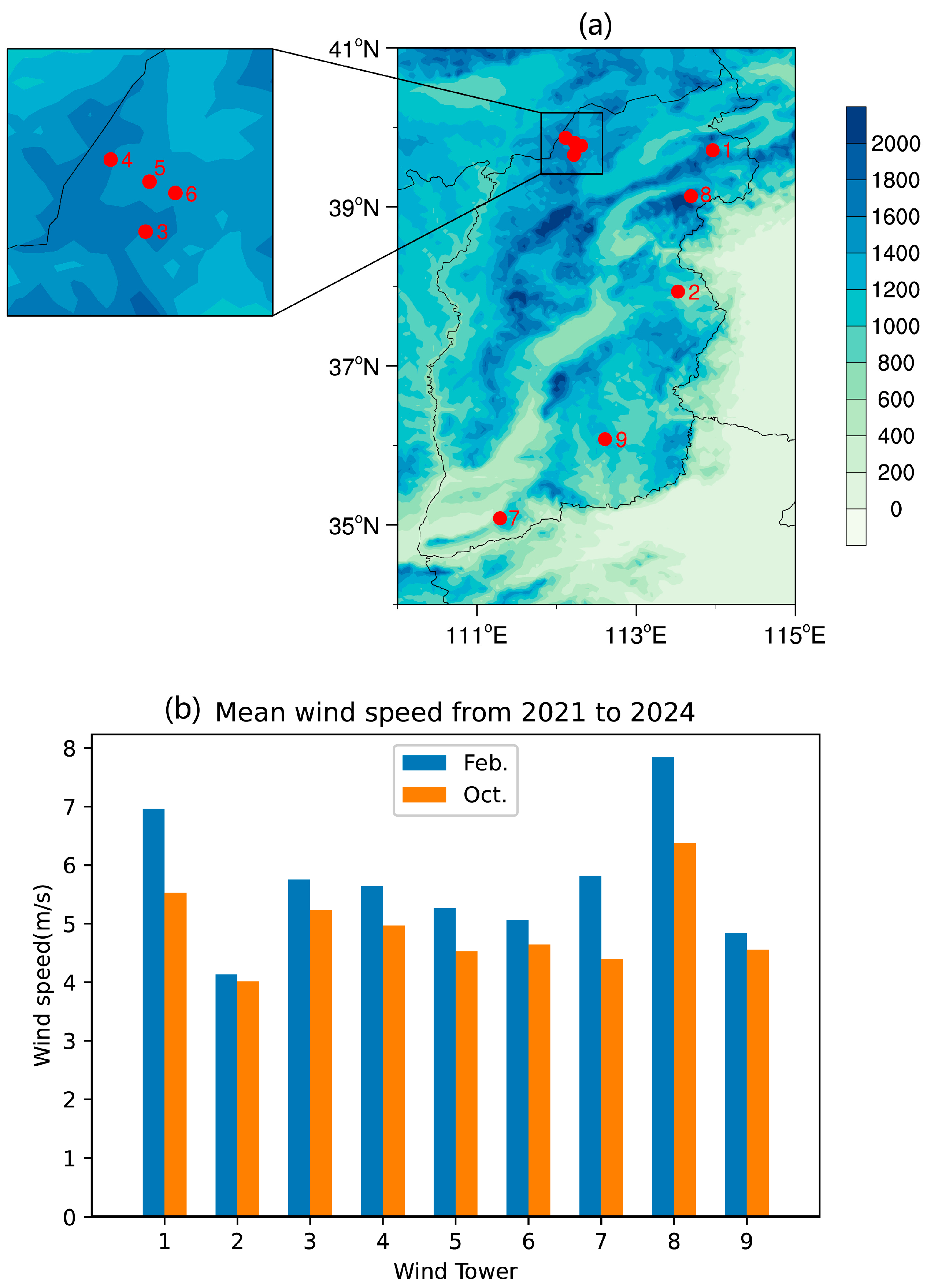
Previous studies have primarily focused on correcting nowcasting predictions (less than 10 days ahead), while research on the applicability of different correction methods to sub-seasonal scales remains notably lacking. This study tries to address these gaps by evaluating three bias correction methods to CFSv2 forecasts in Shanxi. Using high-resolution observational data from nine wind towers (2021–2024), we quantify model biases and assess correction efficacy under different wind speed thresholds and lead times (LTs) extending to 45 days.

This work aims to enhance operational forecasting accuracy and provide insights into the limitations of uniform correction approaches in heterogeneous environments. We select February and October for evaluation, for these two months are the crucial transitional months when the maximum wind speed changes from small to large (or from large to small) [16]. Furthermore, the wind speed variation in these two months has a significant impact on the scheduling and planning of wind power enterprises, but the wind prediction accuracy is lower than other months. Hence, this work mainly focuses on the wind speed prediction correction for these two months, hoping to solve practical problems for wind power enterprises. The data and methods used in this work are introduced in Section 2. Section 3 shows the application effects of the above three methods utilized. A summary and discussion are provided in Section 4.

2. Data and Methods

2.1. Observation and Model Data

Wind speed observation data at 70 m above the land surface from nine wind towers in Shanxi Province in October 2021/2022 and February 2022/2023 are provided as training samples, with a temporal resolution of 15 min. We processed this data into daily averages. The distribution of the nine representative wind towers is shown in Figure 1a. The mean wind speed of nine wind towers from 2021 to 2024 is shown in Figure 1b. Mean wind speeds are greater in February than in October, and wind speeds at higher elevation towers (No. 1 and No. 8) are greater than those at lower elevations.

The ensemble means of hindcasts and real-time predictions initiated from January 1982 to February 2024 from NCEP CFSv2 is examined in this work to investigate the prediction skill and bias correction for near-surface wind speed in Shanxi Province, China. The ensemble means of the real-time predictions includes 40 members within the last 10 days of each month and four forecasts per day, out of 9 months. More details on its operational framework and capabilities can be found in [14], and the model data can be downloaded at https://nomads.ncep.noaa.gov/pub/data/nccf/com/cfs/prod/ (accessed on 4 July 2025).

We used variables of 10 m horizontal wind fields (U and V) for 1–28 February of 2022–2024 and 1–31 October of 2021–2023, and forecasting 1–45 days in advance. The model data includes four members with a temporal resolution of 6 h. Full wind speed forecast data for 1–45 days were calculated from the zonal and meridional wind speeds. Through bilinear interpolation, model grid data were interpolated to the locations of the wind towers. Given that the model’s direct output is limited to 10 m wind speed, we derived 70 m winds by implementing an empirical interpolation algorithm [17] that accounts for the systematic bias between wind tower observation and modeled 10 m winds, with 1.8 serving as the optimal scaling coefficient. Finally, periods with missing measured wind speed data at the wind towers and missing forecast data were removed, organizing a database of 70 m wind speed observations and forecast samples usable for subsequent algorithmic processes. The data from February 2022/2023 and October 2021/2022 are used as training data for the correction model, and the data from February 2024 and October 2023 are used as test data for the evaluation of the correction methods.

Root Mean Square Error (RMSE) is a widely used metric for evaluating the accuracy of predictive models. It measures the average magnitude of the errors between predicted and observed values. Specifically, RMSE is calculated as the square root of the average of the squared differences between the predicted and observed values. Mathematically, it is expressed as

$$RMSE=\sqrt{{\displaystyle \frac{1}{n}}\sum _{i=1}^n{\left(y_{i,pre}-y_{i,obs}\right)}^2}$$

where $y_{obs}$ represents the observed values, $y_{pre}$ represents the predicted values, and “n” denotes the number of observations. The RMSE provides a single measure of predictive accuracy, with lower values indicating better model performance.

2.2. Quantile Regression Method

Quantile Regression (QR) is a statistical method used to estimate the conditional quantiles of the dependent variable based on given values of the independent variable [18]. Unlike traditional Ordinary Least Squares (OLS) regression, which focuses on estimating the conditional mean of the dependent variable, QR provides a more comprehensive analysis by examining various points in the conditional distribution, such as the median, quartiles, and other percentiles.

The basic form of the QR model can be expressed as

$$Q\left(\tau |X=x\right)=x\prime \beta \left(\tau \right)$$

where $Q\left(\tau |X=x\right)$ represents the $\tau$-th quantile of the dependent variable Y given the independent variable $X=x$. The parameter vector $\beta \left(\tau \right)$ is estimated to describe the influence of $X$ on the $\tau$-th quantile of Y.

The parameters $\beta \left(\tau \right)$ are estimated by minimizing the weighted sum of absolute deviations, with the objective function given by

$$min\sum _{i=1}^n{\rho }_{\tau }(Y_i-{X\prime }_i\beta )$$

where ${\rho }_{\tau }\left(u\right)$ is the check function defined as

$${\rho }_{\tau }\left(u\right)=u(\tau -I\left(u\right))$$

and where $u$ is the bias (observed minus predicted value) and $I\left(u\right)$ is the indicator function defined as

$$I\left(u\right)=\left\{\begin{array}{c}1,u<0\\ 0,u\ge 0\end{array}\right.$$

QR is robust to outliers and non-normality in the data, as it does not rely solely on the conditional mean but instead focuses on different parts of the conditional distribution. In addition, by providing estimates at different quantiles, QR offers a more detailed picture of the relationship between the independent and dependent variables.

In this approach, τ = 50 (50th percentile or median) is used for QR correction, following the formula

$${\mathrm{C}\mathrm{o}\mathrm{r}\mathrm{r}\mathrm{e}\mathrm{c}\mathrm{t}}_{\mathrm{Q}\mathrm{R}}={\displaystyle \frac{{\mathrm{Q}\mathrm{R}}_{\mathsf{\tau }=50}+\mathrm{O}\mathrm{r}\mathrm{i}}{2}}$$

where ${\mathrm{C}\mathrm{o}\mathrm{r}\mathrm{r}\mathrm{e}\mathrm{c}\mathrm{t}}_{\mathrm{Q}\mathrm{R}}$ is the result of QR correction, ${\mathrm{Q}\mathrm{R}}_{\mathsf{\tau }=50}$ is the median QR result, and Ori is the original model forecast. ${\mathrm{Q}\mathrm{R}}_{\mathsf{\tau }=50}$ is trained using historical data from the same month in the previous year.

2.3. Linear Regression Method

The Linear Regression (LR) correction method [19] employs a training period similar to that used in QR. The forecast data from the training period serves as the independent variable “x”, while the historical observation data serves as the dependent variable “y”, forming this historical forecast–observation LR correction equation:

$${\mathrm{y}}_{\mathrm{i}}^{\mathrm{*}}=\mathrm{k}{\mathrm{x}}_{\mathrm{i}}+\mathrm{b}$$

where “b” is the intercept of the forecast equation, and ${\mathrm{y}}_{\mathrm{i}}^{\mathrm{*}}$ represents the optimally predicted value through LR.

LR utilizes the least squares method to define the loss function J, which is minimized to derive the optimal forecast–observation LR correction equation. The loss function J is defined as

$$\mathrm{J}=\sum _{\mathrm{i}=1}^{\mathrm{n}}{({\mathrm{y}}_{\mathrm{i}}^{\mathrm{*}}-{\mathrm{y}}_{\mathrm{i}})}^2$$

This method optimizes the parameters “k” (slope) and “b” (intercept) to ensure that the sum of the squared differences between the predicted and observed values is minimized, thereby enhancing the accuracy and reliability of the forecast model.

2.4. Optimal Threat Score Method

The Optimal Threat Score (OTS) correction method [20] is a segmentation correction approach tailored for different thresholds. It utilizes the Threat Score (TS) to optimize forecast corrections. The correction methodology is described as follows:

$${\mathrm{C}\mathrm{o}\mathrm{r}\mathrm{r}\mathrm{e}\mathrm{c}\mathrm{t}}_{\mathrm{O}\mathrm{T}\mathrm{S}}=\left\{\begin{array}{c}0,\mathrm{x}<{\mathrm{F}}_1;\\ {\mathrm{O}}_{\mathrm{k}}+\left({\mathrm{O}}_{\mathrm{k}+1}-{\mathrm{O}}_{\mathrm{k}}\right)\times {\displaystyle \frac{\mathrm{x}-{\mathrm{E}}_{\mathrm{k}}}{{\mathrm{F}}_{\mathrm{k}+1}-{\mathrm{F}}_{\mathrm{k}}}},{\mathrm{F}}_{\mathrm{k}}\le \mathrm{x}<{\mathrm{F}}_{\mathrm{k}+1},\mathrm{k}<\mathrm{n};\\ \mathrm{x}\times {\displaystyle \frac{{\mathrm{O}}_{\mathrm{k}}}{{\mathrm{F}}_{\mathrm{k}}}},\mathrm{x}\ge {\mathrm{F}}_{\mathrm{n}}\end{array}\right.$$

In the formula, “x” and ${\mathrm{C}\mathrm{o}\mathrm{r}\mathrm{r}\mathrm{e}\mathrm{c}\mathrm{t}}_{\mathrm{O}\mathrm{T}\mathrm{S}}$, respectively, represent the forecasted and corrected values of wind speed in the model. ${\mathrm{O}}_{\mathrm{k}}$ is the threshold for the k-th level of wind speed (where k = 1,2,…,n), and ${\mathrm{F}}_{\mathrm{k}}$ denotes the model wind speed threshold that corresponds to the correction up to ${\mathrm{O}}_{\mathrm{k}}$. The smaller (or larger) ${\mathrm{F}}_{\mathrm{k}}$ is relative to ${\mathrm{O}}_{\mathrm{k}}$, the larger (or smaller) the correction coefficient will be. This relationship is crucial for adjusting the forecast to more closely match observed values, thereby improving the accuracy of the model’s predictions.

For a specific threshold, the formula for TS is as follows:

$$TS=N_A/(N_A+N_B+N_C)$$

In the equation, $N_A$ denotes the number of successful wind speed predictions, $N_B$ represents the number of missed forecasts, and $N_C$ indicates the number of false alarms. A higher TS suggests better forecast accuracy for a specific threshold.

3. Results

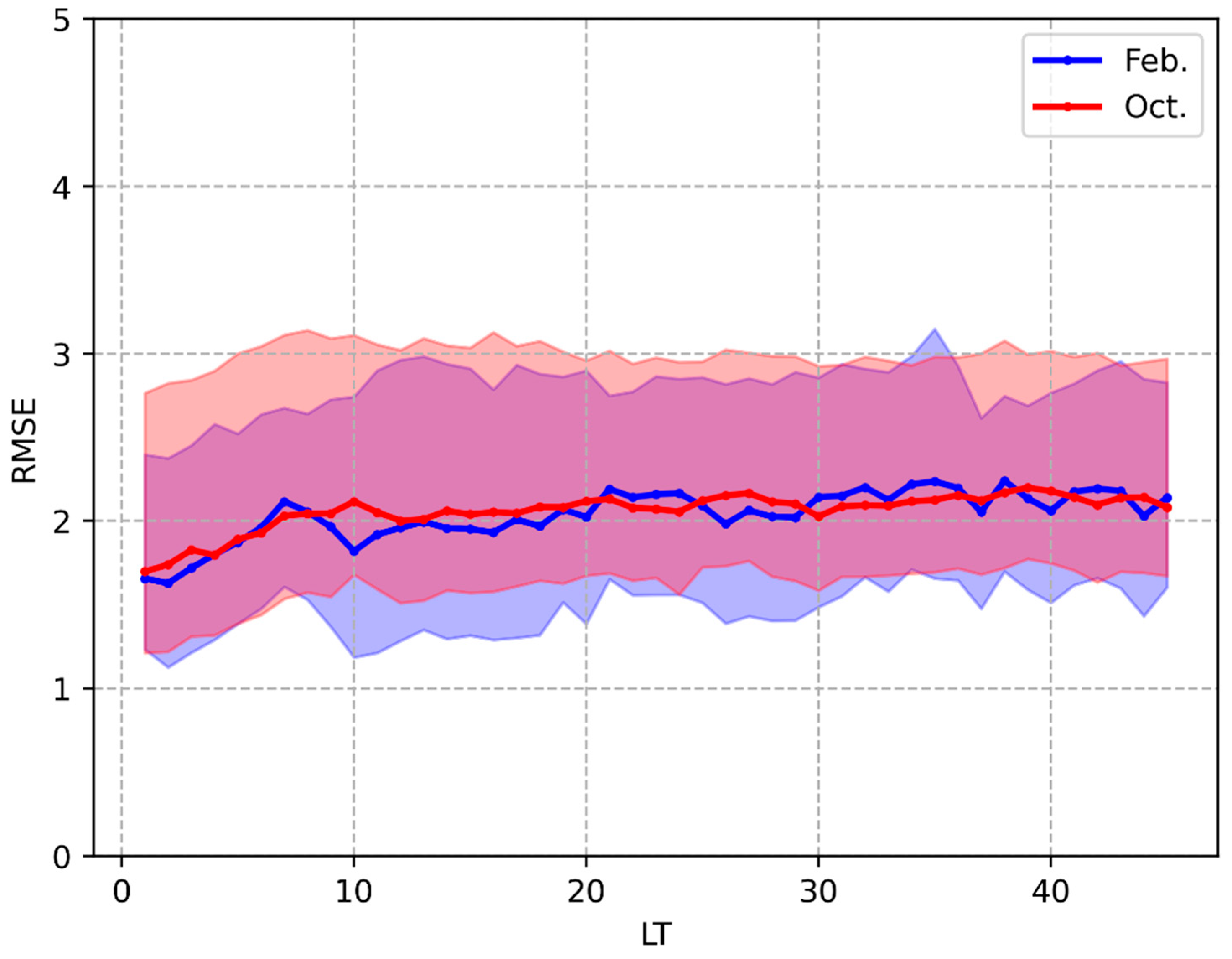
The model bias in February 2022/2023 and October 2021/2022 is shown in Figure 2 and Figure 3. Figure 2 shows the mean RMSE of 70 m wind speed of nine wind towers from 1 to 45 days in advance. The RMSEs of the two months are roughly equivalent, and the variability in February is greater. When the lead time (LT) is less than 7 days, the RMSE increases significantly as the LT increases. For an LT of less than 7 days, the RMSE remains below 2.25 m/s. Subsequently, as the LT extends further, the RMSE fluctuates around an average level above 2.1 m/s. Overall, during the extended forecast period (1 to 45 days in advance), the RMSE of wind speed forecasts exceeds 1.5 m/s, indicating substantial room for improvement in the forecasting performance of the model.

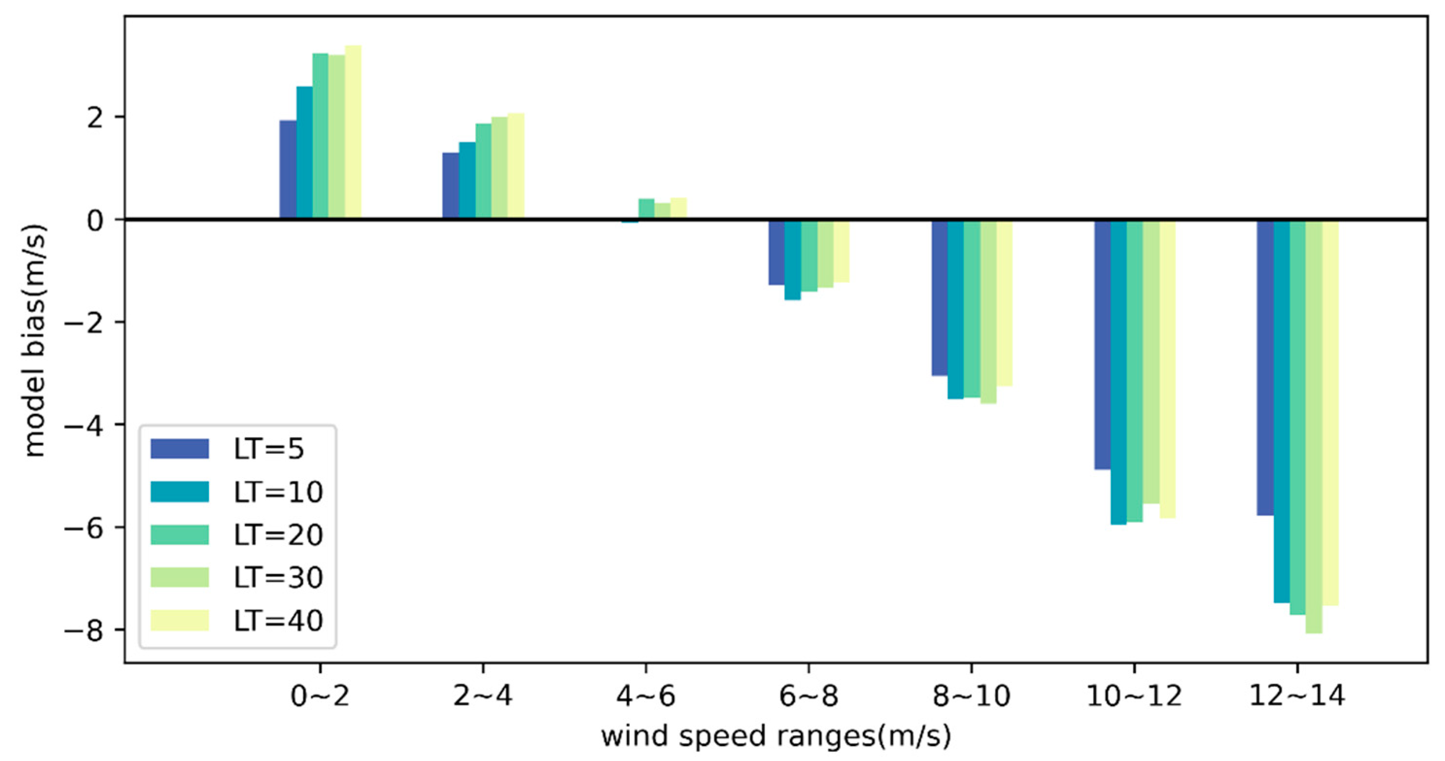
Figure 3 illustrates the average bias of different 70 m wind speed ranges. When the observed 70 m wind speeds are below 6 m/s, the positive model bias occurs in the first three bins. For observed 70 m wind speeds above 6 m/s, a negative model bias is presented, which significantly increases as the wind speed and forecast LT increase. At an LT of 1 day, the model bias for observed wind speeds of 6–8 m/s is −1.5 m/s, and for wind speeds of 12–14 m/s, the average bias is −5.6 m/s. When the LT extends to 30 days, the model bias remains at −1.6 m/s with observed wind speeds of 6–8 m/s, but the bias for wind speeds of 12–14 m/s reaches −7.7 m/s. It is implied that the model demonstrates a distinct bias characteristic for 70 m wind speed forecasts, with underestimation for higher wind speeds and overestimation for lower wind speeds, which is similar to a previous study [21].

For the low prediction skill of the model for 70 m wind speed (Figure 2), and based on the characteristics of model bias within different wind speed ranges (Figure 3), three bias correction methods are selected to attempt to reduce model bias and improve the prediction accuracy of wind speed.

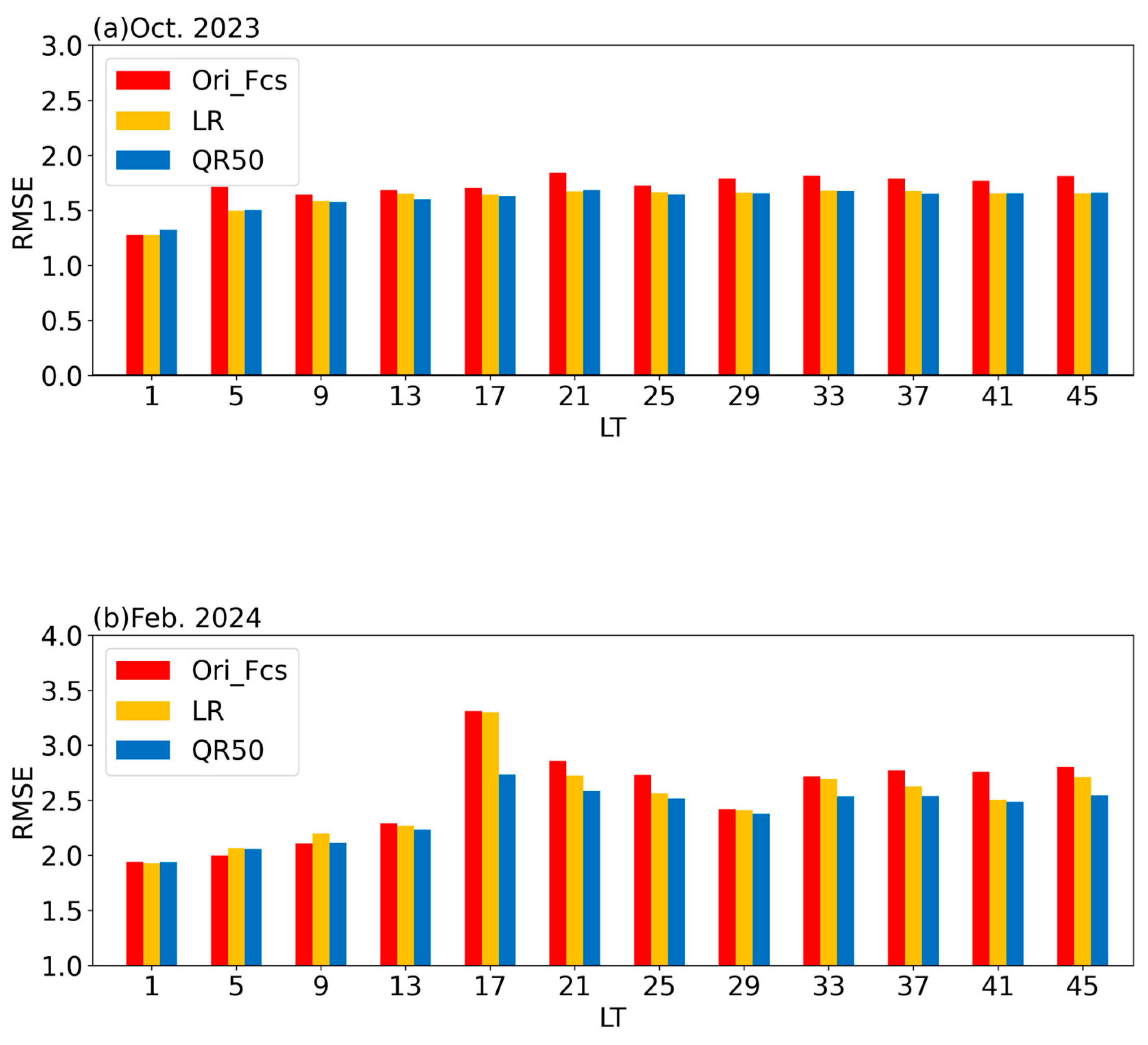
To evaluate the overall bias levels under different correction methods, the RMSE of the original model forecast is calculated for the test periods (October 2023 and February 2024). The corresponding RMSEs before and after correction are shown in Figure 4 and summarized in

Table 1. Mean RMSE at each wind tower under different bias correction methods in October 2023 and February 2024. The RMSE in the table is calculated by averaging RMSEs of all lead times and all target days.

	Wind Tower	1	2	3	4	5	6	7	8	9	Mean RMSE
October 2023	Ori_Fcs	1.40	1.42	1.22	1.29	1.43	1.43	1.78	2.52	1.12	1.52
	LR	1.28	1.36	0.98	0.97	0.94	1.04	2.11	2.57	1.08	1.37
	OTS	1.43	1.48	1.29	1.35	1.49	1.48	1.76	2.54	1.18	1.56
	QR50	1.27	1.35	1.01	1.00	1.04	1.12	1.88	2.55	1.05	1.36
February 2024	Ori_Fcs	2.08	2.28	2.11	2.14	2.26	2.46	3.77	2.43	1.62	2.35
	LR	1.95	2.30	2.01	2.05	2.17	2.37	3.48	2.35	1.65	2.26
	OTS	2.18	2.33	2.22	2.25	2.37	2.56	3.93	2.50	1.70	2.45
	QR50	1.76	2.18	1.82	1.86	1.91	2.11	3.48	2.34	1.50	2.11

. After applying three different correction methods, the results indicate that the OTS method does not effectively reduce forecast bias, suggesting that a uniform correction coefficient based on different thresholds is not suitable in cases where there is significant bias variability across wind towers. In contrast, the other two correction methods successfully reduce the model bias at all wind towers, except for wind towers 7 and 8 in October 2023, demonstrating the robustness of using historical data for regression-based forecast corrections, particularly at wind towers with high original RMSE. The QR50 method is notably effective in the two test periods.

Wind tower 9, which has the lowest RMSE among all the wind towers, also shows a significant reduction (more than a 6% reduction in model bias across both periods) of mean RMSE with the QR50 method. From an average perspective across all the wind towers, during October 2023 (February 2024), the QR50 method reduces the original RMSE from 1.52 (2.35) to 1.36 (2.11) as in Table 1, a decrease of 11% (10%), passing the 95% student-t significant test.

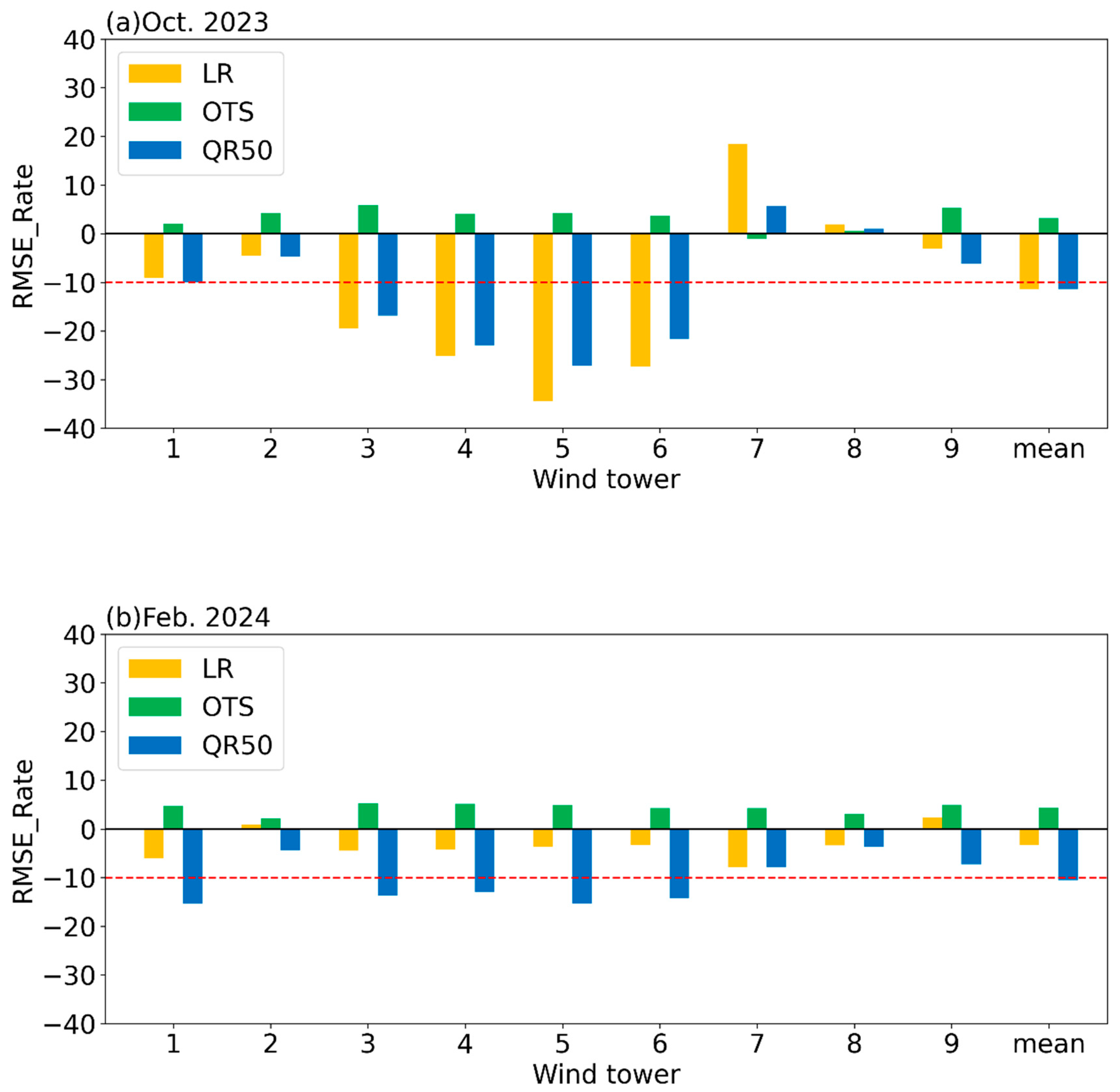
Figure 5 presents the growth rate of the RMSE (RMSE_rate, defined as the difference between the RMSE after correction and before correction, divided by the RMSE before correction) for the three correction methods. The mean RMSE_Rate of the three methods is −3.28%, 4.33%, and −10.50%, respectively, in October 2023 (Figure 5a) and −11.38%, 3.21%, and −11.40%, respectively, in February 2024 (Figure 5b). Overall, the OTS method has an opposite correction effect, which can increase the RMSE by approximately 5% (green bars in Figure 5). In October 2023, the LR method effectively reduced the RMSE across all stations except for wind towers 7 and 8. Notably, the reduction exceeded 10% at wind towers 3, 4, 5, and 6, with the most significant improvement observed at wind tower 5, where the reduction surpassed 30% (yellow bars in Figure 5a). The QR50 method demonstrated a reduction in the RMSE across all stations except for wind towers 8 and 9. However, the magnitude of reduction was generally smaller compared to the LR method. Notably, at wind towers 3, 4, 5, and 6, the reduction exceeded 10%, with wind tower 5 showing the most significant improvement, where the reduction surpassed 25% (blue bars in Figure 5a). The reduction in the RMSE achieved by both the LR and QR50 methods is less significant in February 2024 (Figure 5b) compared to October 2023 (Figure 5a). Only the QR50 method achieved a reduction in the RMSE exceeding 10% at wind towers 1, 3, 4, 5, and 6 (blue bars in Figure 5b). When the RMSE values are higher (with the February 2024 RMSE generally exceeding 2 in Figure 4b), the QR50 method demonstrates a more stable correction performance compared to the LR method.

Next, we conducted a comparative analysis of the performance of QR50 and LR methods across various LTs in Figure 6. In October 2023 (Figure 6a), both the LR and QR50 methods reduced the RMSE in varying degrees across all LTs except for short LTs (1–4 days). At longer LTs, the magnitude of RMSE reduction increased significantly, while the two methods exhibited comparable performance. In February 2024 (Figure 6b), both correction methods failed to reduce the RMSE across LTs of 1–9 days. They slightly increased the RMSE at 5-day and 9-day LTs. When the LT exceeded 10 days, both methods effectively reduced the RMSE, and the magnitude of reduction shows a slight increase as the LT extended further. The QR50 method consistently demonstrates superior RMSE reduction compared to the LR method, particularly under conditions of higher RMSE values. For instance, at a 17-day LT, the LR method shows a minimal reduction in the RMSE, while the QR50 method achieves substantial RMSE reduction. The analysis reveals that the correction methods primarily reduce the RMSE at LTs exceeding 10 days. Furthermore, the correction effectiveness improves as the LT increases. Notably, under conditions of higher RMSE, the QR50 method demonstrates a more stable correction performance compared to the LR method.

To further investigate the reasons behind the varying correction performance of different methods across wind towers, we selected wind tower 5 (Figure 7), which demonstrated the best correction performance in October 2023, and wind tower 7 (Figure 8), which exhibited the poorest correction performance, for detailed analysis.

In October 2023, the daily wind speeds at wind tower 5 exhibited minor fluctuations around 4 m/s, as indicated by the black solid line in Figure 7. At an LT of 1 day, the raw CFSv2 predictions effectively capture the characteristics of daily wind speed variations. Both correction methods show minimal differences compared to the raw model output for most periods. However, slight adjustments are observed under specific conditions: the methods correct lower wind speeds upward (e.g., around 2 m/s on October 10) and higher wind speeds downward (e.g., around 8 m/s on October 31). Consequently, the overall RMSE remains largely unchanged, as illustrated in Figure 6a. At an LT of 5 days, the CFSv2 model continues to capture the intra-monthly variation characteristics of wind speed. However, it significantly underestimates the wind speeds during the early and mid-to-late periods of the month, exhibiting a tendency to overestimate low wind speeds and underestimate high wind speeds. Both the QR50 and LR methods demonstrate effective correction capabilities under these conditions.

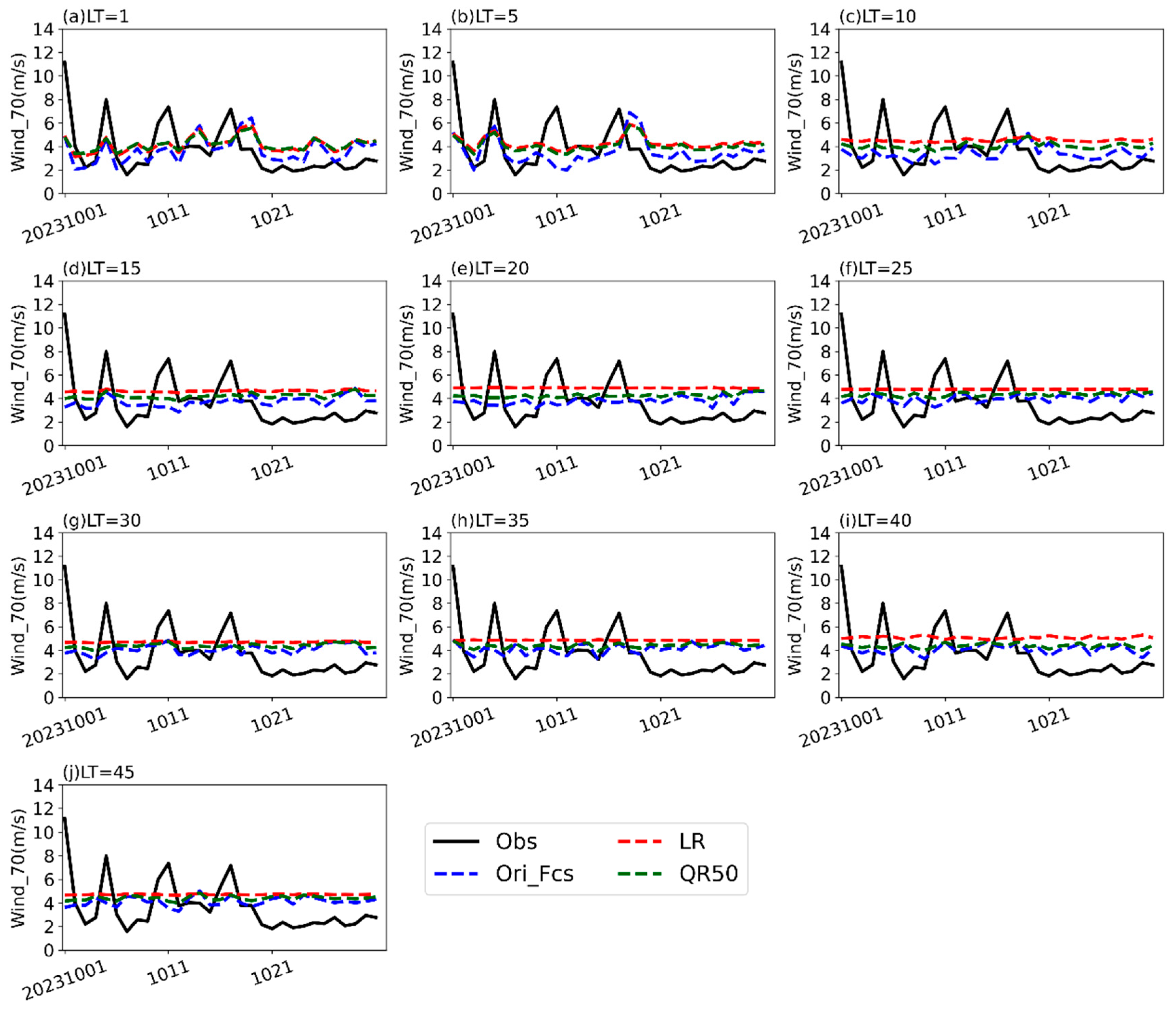
In October 2023, four high-wind events were recorded at wind tower 7 compared to wind tower 5, with daily average wind speeds exceeding 11, 8, 7, and 7 m/s, respectively (black lines in Figure 8). The original forecasts from the CFSv2 model demonstrate relatively accurate capture of the first two high-wind events at an LT of less than 10 days. However, for the third and fourth high-wind events, the predictions exhibit a lag of approximately 2 days (blue lines in Figure 8). After October 20th, the observed wind speed fluctuated at around 2 m/s, while the wind speed predicted by CFSv2 exhibits a systematic positive bias, consistently overestimating the actual values. At an LT greater than 10 days, the model predicted wind speed exhibits minimal intra-monthly variability, remaining consistently around 4 m/s. This suggests a significant loss of predictive skill in capturing temporal wind speed fluctuations at extended forecast ranges, highlighting a limitation in the model’s ability to resolve small-scale atmospheric dynamics over longer LTs. The QR50 and LR methods exhibit a tendency to adjust wind speeds upward, which demonstrates a positive correction effect during several high-wind events. However, during intermittent periods of high winds, particularly in late October, this correction leads to an increase in the RMSE.

Next, we analyzed two wind towers with contrasting correction performance in February 2024: wind tower 1 (Figure 9), which demonstrates relatively effective correction results, and wind tower 8 (Figure 10), which exhibits comparatively poor correction performance. This comparative analysis aims to identify the factors contributing to the differential effectiveness of the correction methods and to explore potential improvements in forecasting accuracy.

For wind tower 1, the wind speed in February exhibits a trend of initially increasing and subsequently decreasing (black lines in Figure 9). At an LT of less than 15 days, the CFSv2 model demonstrates a relatively good ability to capture the intra-monthly variations in wind speed, particularly for the two high-wind events around the 11th and 15th, with wind speeds approaching 10 m/s (Figure 9a–d). However, the model significantly overestimates wind speeds around the 8th and 18th. Both the QR50 and LR methods slightly reduce the overestimated wind speeds, thereby decreasing the RMSE. At an LT greater than 15 days, the CFSv2 model largely fails to capture the intra-monthly variations in wind speed, resulting in overestimated wind speeds in the first 10-day period, underestimated wind speeds in the middle 10-day period, and overestimated wind speeds again in the last 10-day period. The QR50 and LR methods primarily adjust the predicted wind speeds downward in the first 10-day period and last 10-day period, thereby reducing the overall RMSE.

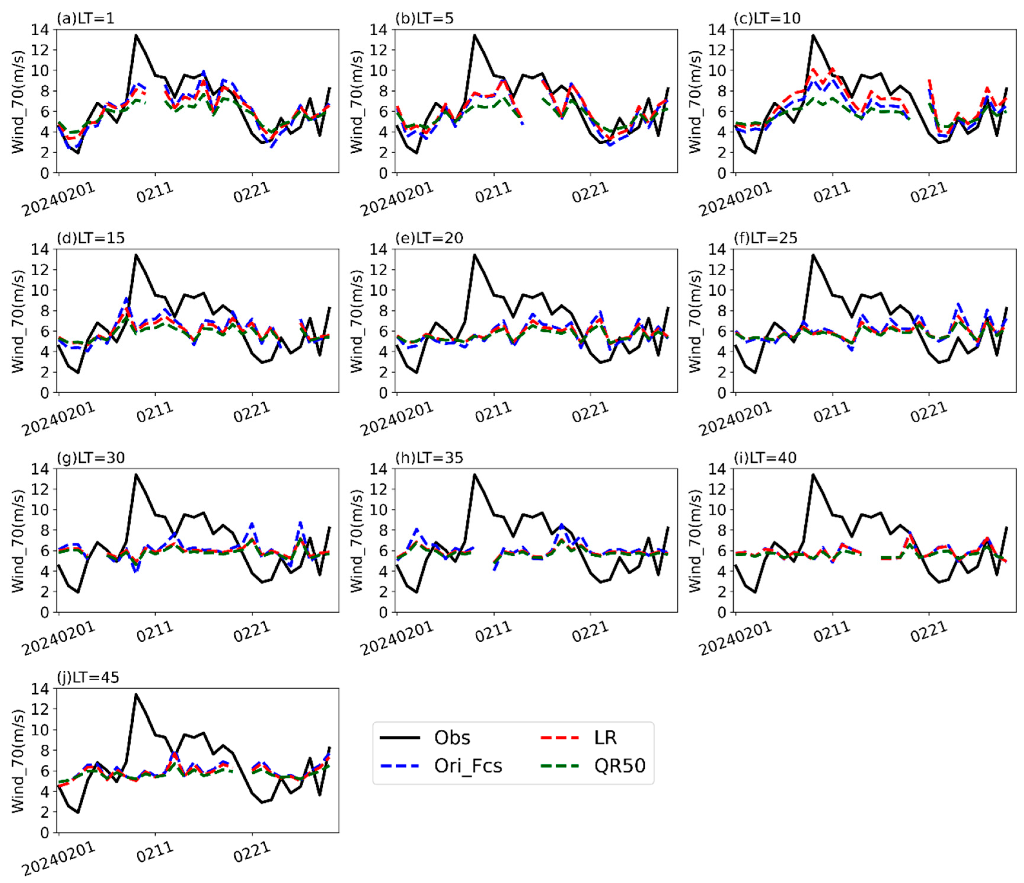
For February 2024, the wind speed at wind tower 8 exhibits a trend of initially increasing, then decreasing, followed by fluctuations toward the end of the month (black lines in Figure 10). At an LT of less than 15 days, the CFSv2 generally captures the intra-monthly variations in wind speed. However, it significantly underestimates the magnitude of the extreme high-wind event on the 9th, with observed wind speeds exceeding 13 m/s but predicted speeds reaching only 8 m/s (Figure 10a–d). Due to the absence of similar cases in the training period during February, both the QR50 and LR methods adjust wind speeds downward during the high-wind event, resulting in an increase in the RMSE. At an LT greater than 15 days, the CFSv2 model overestimates wind speeds from the 1st to the 3rd, underestimates wind speeds from the 8th to the 18th, and overestimates wind speeds from the 19th to the 22nd (Figure 10e–j). Influenced by the extreme wind speeds, neither correction method is able to effectively adjust the wind speeds, leading to a relatively large RMSE during this period.

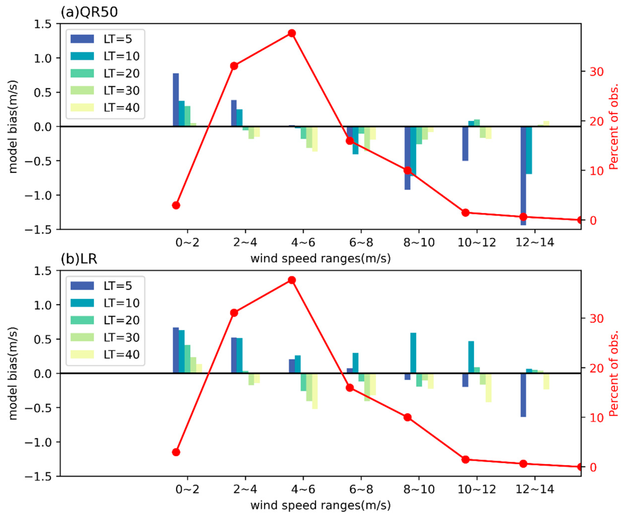
The differences of bias between post-corrected and before-corrected results in different wind speed bins are presented in Figure 11. From the figure, we can see that our correction method works mainly when the LT is large, consistent with the final results. What is more, the correction can reduce ‘smaller wind speeds’ mainly from 2 m/s to 8 m/s, but it performs poorly for larger wind speeds except for LR at LT = 10. The probability density distribution of wind speeds (red lines on the right y-axis) shows that the wind speeds are mainly distributed in the range of 2–8 m/s (each interval is more than 10%), and the improvement in our correction method for the wind speeds in the main wind speed distribution intervals leads to the final results.

4. Summary and Discussion

This study evaluates the prediction performance of the CFSv2 model for wind speeds at a height of 70 m at nine wind towers in Shanxi Province during February and October. The results indicate that the CFSv2 model consistently overestimates low wind speeds (<6 m/s) and underestimates high wind speeds (>6 m/s), with RMSE exceeding 1.5 m/s. Biases amplify with LT increases, reaching −7.7 m/s for 12–14 m/s winds at 30-day LTs.

To improve the model performance, three correction schemes were tested to correct the 70 m wind speed simulations. QR50 outperformed the other methods, reducing the mean RMSE by ~10% in both test periods. Its robustness stems from addressing conditional distribution biases, particularly at longer LTs (>10 days). LR showed significant improvements in October 2023 but less stability in February 2024, suggesting sensitivity to seasonal variability. OTS increased the RMSE by ~5%, failing to account for spatial heterogeneity across wind towers. QR50′s effectiveness supports its integration into operational forecasting systems, especially for extended LTs. These findings highlight the potential of statistical correction methods, especially QR50, in enhancing the accuracy of wind speed forecasts under varying meteorological conditions.

The reduction in the RMSE by the QR50 and LR methods is primarily observed at LTs greater than 10 days, with minimal impact on the RMSE at LTs of less than 10 days. This is largely attributed to the model’s relatively accurate prediction of intra-monthly wind speed variations at LTs of less than 10 days, particularly its ability to capture high-wind events, albeit with insufficient magnitude. In contrast, at LTs greater than 10 days, the model’s predicted intra-monthly wind speed variations exhibit reduced amplitude, allowing the correction methods to amplify or reduce wind speeds based on historical data, thereby better capturing the observed wind speed variations. When intra-monthly wind speed variations are relatively small, the correction methods demonstrate a more pronounced reduction in the RMSE. However, during periods with high-wind events, the lack of corresponding historical records for such extreme conditions leads to poorer correction performance. This underscores the importance of historical data representativeness and the challenges in correcting forecasts for rare or extreme meteorological events. Extreme wind events (e.g., >13 m/s at wind tower 8) highlight the limitations of regression methods when historical training data lacks analogous cases.

Due to the relatively short observation period in the wind towers, we modeled for different months and different LTs, with no distinction between wind towers, leading to incomplete consideration of the characteristics of different wind towers as well as a few extremely high-wind events which were observed and therefore included in the correction methods. Thus, future work should explore hybrid methods combining QR50 with machine learning to address extreme events and improve temporal resolution [22]. Additionally, expanding training datasets to include diverse meteorological conditions could enhance model generalizability. Moreover, factors such as the topography and environmental conditions surrounding each anemometer tower should be considered in the development of tailored correction approaches [23]. These considerations are critical for improving the adaptability and precision of correction methods across diverse geographical and meteorological contexts.

References

1. Zhang, X.D. Overview of wind energy resources and wind power development in Shanxi. Shanxi Electr. Power 2009, 2009, 4. [Google Scholar] [CrossRef]
2. Wang, A.; An, L. The problems of and suggestions on wind power generation in Shanxi Province. Shanxi Electr. Power 2011, 2011, 9–11. [Google Scholar]
3. Alessandrini, S.; Delle Monache, L.; Sperati, S.; Nissen, J.N. A novel application of an analog ensemble for short-term wind power forecasting. Renew. Energy 2015, 76, 768–781. [Google Scholar] [CrossRef]
4. Shi, J.; Liu, Y.; Li, Y.; Liu, Y.; Roux, G.; Shi, L.; Fan, X. Wind speed forecasts of a mesoscale ensemble for large-scale wind farms in Northern China: Downscaling effect of global model forecasts. Energies 2022, 15, 896. [Google Scholar] [CrossRef]
5. Döscher, R.; Acosta, M.; Alessandri, A.; Anthoni, P.; Arsouze, T.; Bergman, T.; Bernardello, R.; Boussetta, S.; Caron, L.-P.; Carver, G.; et al. The EC-Earth3 Earth system model for the Coupled Model Intercomparison Project 6. Geosci. Model Dev. 2022, 15, 2973–3020. [Google Scholar] [CrossRef]
6. Tseng, B.; Garcia, C.; Kwon, J. Optimization of wind turbine placement layout on non-flat terrains. Int. J. Ind. Eng. Theory Appl. Pract. 2014, 21, 384–395. [Google Scholar]
7. Bauer, P.; Thorpe, A.; Brunet, G. The quiet revolution of numerical weather prediction. Nature 2015, 525, 47–55. [Google Scholar] [CrossRef]
8. Bauer, P. What if? Numerical weather prediction at the crossroads. J. Eur. Meteorol. Soc. 2024, 1, 100002. [Google Scholar] [CrossRef]
9. Peng, X.; Che, Y.; Chang, J. A novel approach to improve numerical weather prediction skills by using anomaly integration and historical data. J. Geophys. Res. Atmos. 2013, 118, 8814–8826. [Google Scholar] [CrossRef]
10. Han, L.; Chen, M.; Chen, K.; Chen, H.; Zhang, Y.; Lu, B.; Song, L.; Qin, R. A deep learning method for bias correction of ECMWF 24-240 h forecasts. Adv. Atmos. Sci. 2021, 38, 1444–1459. [Google Scholar] [CrossRef]
11. Chen, Y.; Lin, H. Overview of the development of offshore wind power generation in China. Sustain. Energy Technol. Assess. 2022, 53, 102766. [Google Scholar] [CrossRef]
12. Sweeney, C.P.; Lynch, P.; Nolan, P. Reducing errors of wind speed forecasts by an optimal combination of post-processing methods. Meteorol. Appl. 2013, 20, 32–40. [Google Scholar] [CrossRef]
13. Sun, L.; Lan, Y.; Sun, X.; Liang, X.; Wang, J.; Su, Y.; He, Y.; Xia, D. Deterministic forecasting and probabilistic post-processing of short-term wind speed using statistical methods. J. Geophys. Res. Atmos. 2024, 129, e2023JD040134. [Google Scholar] [CrossRef]
14. Saha, S.; Moorthi, S.; Wu, X.; Wang, J.; Nadiga, S.; Tripp, P.; Behringer, D.; Hou, Y.-T.; Chuang, H.-Y.; Iredell, M.; et al. The NCEP climate forecast system version 2. J. Clim. 2014, 27, 2185–2208. [Google Scholar] [CrossRef]
15. Gandoin, R.; Garza, J. Underestimation of strong wind speeds offshore in ERA5: Evidence, discussion and correction. Wind Energy Sci. 2024, 9, 1727–1745. [Google Scholar] [CrossRef]
16. Zhang, G.; Azorin-Molina, C.; Chen, D.; Guijarro, J.A.; Kong, F.; Minola, L.; McVicar, T.R.; Son, S.-W.; Shi, P. Variability of daily maximum wind speed across China, 1975–2016: An examination of likely causes. J. Clim. 2020, 33, 2793–2816. [Google Scholar] [CrossRef]
17. Ren, L.; Yang, Y.; Wang, H.; Wang, P.; Yue, X.; Liao, H. Co-benefits of mitigating aerosol pollution to future solar and wind energy in China toward carbon neutrality. Geophys. Res. Lett. 2024, 51, e2024GL109296. [Google Scholar] [CrossRef]
18. Liu, P.; Zhou, J.; Tan, C. Quantile regression analysis of the number of urban fires and meteorological factors. J. Hefei Univ. Technol. (Nat. Sci.) 2013, 36, 1273–1277. [Google Scholar] [CrossRef]
19. Yin, Y.; Wu, L.; Yan, R.; Ma, H.; Liu, C. Study on regression approaches of extending daily temperature extremes for local weather stations and the error analysis. Meteorol. Environ. Sci. 2023, 46, 95–103. [Google Scholar] [CrossRef]
20. Wu, Q.; Han, M.; Liu, M.; Chen, F. A comparison of optimal score-based correction algorithms for model precipitation prediction. J. Appl. Meteorol. Sci. 2017, 28, 306–317. [Google Scholar] [CrossRef]
21. Pan, L.; Liu, Y.; Roux, G.; Cheng, W.; Liu, Y.; Hu, J.; Jin, S.; Feng, S.; Du, J.; Peng, L. Seasonal variation of the surface wind forecast performance of the high-resolution WRF-RTFDDA system over China. Atmos. Res. 2021, 259, 105673. [Google Scholar] [CrossRef]
22. Alves, D.; Mendonça, F.; Mostafa, S.S.; Morgado-Dias, F. Deep learning enhanced wind speed and direction forecasting for airport regions. Weather Forecast. 2025, 40, 207–221. [Google Scholar] [CrossRef]
23. Koo, J.; Han, G.D.; Choi, H.J.; Shim, J.H. Wind-speed prediction and analysis based on geological and distance variables using an artificial neural network: A case study in South Korea. Energy 2015, 93, 1296–1302. [Google Scholar] [CrossRef]
Figure 1. (a) Distribution of nine wind towers in Shanxi Province, China. The shaded areas represent elevation levels (unit: m). (b) The mean wind speed of nine wind towers from 2021 to 2024.
Climate 13 00150 g001
Figure 2. Mean RMSE (y-axis) of wind speed observed by nine wind towers with different LTs (x-axis) in October of 2021/2022 and February of 2022/2023. The shadow represents the range between upper 90% and lower 10%.
Climate 13 00150 g002
Figure 3. Model biases with different ranges of 70 m wind speed (color bars represent forecasts with LT of 5, 10, 20, 30, and 40 days).
Climate 13 00150 g003
Figure 4. Mean RMSE (y-axis) across different wind towers (x-axis) in (a) October 2023, respectively) and (b) February 2024. The different color bars represent different correction methods and the original model output. The RMSE is calculated by averaging RMSEs of all lead times and all target days in a wind tower.
Climate 13 00150 g004
Figure 5. RMSE_Rate (%) (y-axis) across different wind towers (x-axis) under different correction methods in (a) October 2023 and (b) February 2024.
Climate 13 00150 g005
Figure 6. Mean RMSE (y-axis) with different lead days (x-axis) under various correction methods in (a) October 2023 and (b) February 2024.
Climate 13 00150 g006
Figure 7. The daily 70 m wind speeds at wind tower 5 are analyzed based on observations from the wind tower (black solid line), CFSv2 output (blue dashed line), LR correction method (red dashed line), and QR50 correction method (dark green dashed line) at LTs of (a) 1 day, (b) 5 days, (c) 10 days, (d) 15 days, (e) 20 days, (f) 25 days, (g) 30 days, (h) 35 days, (i) 40 days, and (j) 45 days.
Climate 13 00150 g007
Figure 8. The daily 70 m wind speeds at wind tower 7 are analyzed based on observations from the wind tower (black solid line), CFSv2 output (blue dashed line), LR correction method (red dashed line), and QR50 correction method (dark green dashed line) at LTs of (a) 1 day, (b) 5 days, (c) 10 days, (d) 15 days, (e) 20 days, (f) 25 days, (g) 30 days, (h) 35 days, (i) 40 days, and (j) 45 days.
Climate 13 00150 g008
Figure 9. The daily 70 m wind speeds at wind tower 1 in February 2024 are analyzed based on observations from the wind tower (black solid line), CFSv2 output (blue dashed line), LR correction method (red dashed line), and QR50 correction method (dark green dashed line) at LTs of (a) 1 day, (b) 5 days, (c) 10 days, (d) 15 days, (e) 20 days, (f) 25 days, (g) 30 days, (h) 35 days, (i) 40 days, and (j) 45 days.
Climate 13 00150 g009
Figure 10. The daily 70 m wind speeds at wind tower 8 in February 2024 are analyzed based on observations from the wind tower (black solid line), CFSv2 output (blue dashed line), LR correction method (red dashed line), and QR50 correction method (dark green dashed line) at LTs of (a) 1 day, (b) 5 days, (c) 10 days, (d) 15 days, (e) 20 days, (f) 25 days, (g) 30 days, (h) 35 days, (i) 40 days, and (j) 45 days.
Climate 13 00150 g010
Figure 11. The difference of bias between post-corrected and before-corrected results in different wind speed bins (bias after correction minus bias before correction) using (a) RQ50 and (b) LR method. The red lines on the right y-axis represent the probability (%) of the wind speed in each bin.
Climate 13 00150 g011