Abstract
The assessment of the maximum snow-water equivalent in mountains is important for understanding the mechanism of their formation, as well as for hydrological calculations. The low density of the observation network and the high complexity of ground-based snow-measuring operations have led to the widespread use of remote methods to obtain such data. In this study, the maximum water reserve of the Uba River basin was calculated for the period of 2020–2023, based on data from the Sentinel-2 satellite regarding the position of the seasonal snow line, obtained using the temperature-based melt-index method. This study determined the snowmelt coefficients for the meteorological stations at Zmeinogorsk, Shemonaikha, and Ridder. Maps were constructed to show the distribution of the maximum snow-water equivalent in the Uba River basin. The spatial differentiation features of the snow cover were revealed, depending on the elevation, slope exposure, and distance from the watersheds. It was established that the altitudinal distribution of snow cover on the northern and southern macro-slopes of the ridges is asymmetric: in the western part of the basin, within the elevation range of 500–1200 m, the maximum water reserves of snow cover are greater on the southern slopes, but they become higher on the northern slopes above 1200 m. In the eastern part of the basin, they are always larger on the northern slopes. The greatest differences in the distribution of snow cover between the slopes occur near the watersheds.
1. Introduction
Snow cover is an important factor in the functioning of geosystems [1]. It affects the climate, relief (terrain), hydrological and soil formation processes, and the lives of plants and animals. Due to its high albedo, snow cover significantly reduces the shortwave radiation reaching the Earth’s surface. At the same time, it decreases the heat exchange between the ground and the atmosphere, reducing the heat loss into the atmosphere and thereby diminishing soil freezing and temperature fluctuation amplitudes within it. However, snow itself is an effective emitter and loses a significant amount of heat in the form of longwave radiation. During spring, a considerable portion of the incoming heat is used for snowmelt, while snow cover slows the transfer of heat into the soil. Snow cover plays a crucial role in the water cycle. The water reserves contained within it influence the soil’s water regime. Snowmelt contributes significantly to river runoff in regions where snow cover forms. It determines the annual runoff volume, the level of spring floods, the ice regime of rivers, the intensity of ice formation and avalanche processes, and the annual balance of glaciers. The study of snow cover is especially relevant in the context of global climate change and the need to forecast hazardous natural phenomena such as avalanches, mudflows, floods, and others [2,3,4,5].
However, snow-cover data are often insufficient for such forecasting due to the local observation via meteorological services. The situation is especially aggravated in mountains, where the number of factors affecting the distribution of snow cover (elevation above sea level, exposure, slopes, orientation of ridges relative to the transport of air masses, etc.) and, consequently, the complexity of ground snow-measuring operations increases significantly.
The widespread development of remote sensing of the Earth partially addresses this issue. Satellite images at least allow for an assessment of the phenological state of the snow cover and its position on a particular date [6,7,8]. From there, it is possible to derive quantitative indicators of snow cover—its establishment and melting in a specific area, the duration of its presence, and, finally, its water reserves. In recent decades, various automated snow cover-mapping methods have been developed that greatly simplify data analysis and improve the accuracy of results, allowing the efficient extraction of snow-cover information from satellite data. The main methods include optical, radar, lidar, and hybrid approaches.
Spectral analysis-based methods (optical) rely on analyzing the spectral characteristics of snow in the visible and near-infrared ranges, enabling the efficient identification of snow cover in satellite images [9,10,11,12]. The most commonly used data sources are optical images from Landsat and Sentinel satellites [13,14,15,16,17].
Synthetic aperture radar (SAR) satellite images, such as those from Sentinel-1, allow for effective snow-cover mapping, especially under cloudy conditions where optical methods are less effective. SAR imagery provides information on snow depth and density, which is crucial for assessing water resources [18,19,20,21,22,23,24].
Lidar (light detection and ranging) technology uses laser pulses to measure distances to the Earth’s surface. This method allows one to obtain highly accurate data on the depth of snow cover and its structure. Lidar data can be used to create three-dimensional models of snow cover and analyze its changes over time [25,26,27,28].
Combining different approaches, such as optical and radar data, can significantly improve the accuracy of mapping. Hybrid methods make it possible to use the advantages of each approach and compensate for their disadvantages [29,30].
Modern machine learning algorithms used to automate the process of snow-cover classification significantly improve the accuracy of mapping. With the application of neural networks and other methods, models can be trained based on historical data, which improves the accuracy and speed of mapping [31,32,33,34,35].
Automated snow-cover-mapping methods offer several advantages, such as a high data-processing speed, the ability to cover large areas, and the minimization of subjective errors. However, there are also limitations to using such data and methods, including dependence on image quality and resolution, difficulties in distinguishing snow under cloudy conditions or in vegetated areas, and the need for calibration and validation based on ground-based data. The use of satellite imagery for snow-cover mapping and dynamic analysis began with the launch of the Landsat missions and the Multispectral Scanner (MSS) satellite. Currently, ready-made products for analyzing snow-cover time series are also available, such as those based on daily MODIS data. The use of MODIS data from the Terra/Aqua satellites is highly popular in snow-cover research due to their daily temporal resolution [36,37,38,39,40,41,42,43]. The Terra and Aqua satellites orbit the Earth and cross the equator approximately every three hours, increasing the likelihood of acquiring cloud-free images. Snow-cover data products based on MODIS data from the Terra (MOD10A2) and Aqua (MYD10A2) satellites provide an eight-day composite with a spatial resolution of 500 m, containing information on maximum snow cover during the compositing period [44].
There are many approaches used to calculate the maximum water reserves of snow cover, but the most common are the energy-balance method and the temperature-based melt-index method. Using the energy-balance method, it is possible to calculate the amount of snow melting at the snow/air interface based on many indicators [45], considering the processes of heat and moisture exchange between the atmosphere and snow and between snow and soil, as well as the processes occurring in the snow layer. Many models have been developed based on this method [46,47]. However, the balance method for calculating snow melting also has its limitations and requires additional parameters that are not always measured instrumentally.
The temperature-based melt-index method uses air temperature as the sole indicator of energy exchange at the snow surface [48,49]. Many researchers recognize the effectiveness of this method, as air temperature correlates with many elements of the energy balance [50,51,52], essentially functioning as a proxy for them. The first attempts to justify melt rates based on air temperature were made in studies explaining the elevation of glaciation [53,54]. In the USSR, this approach was first applied by [55], and later, other Soviet researchers explored it [56]. Today, the method continues to be used for hydrological and glaciological purposes [51,57,58,59], including in the Altai region [60]. The essence of this method is that a certain sum of air temperatures is required to melt a specific amount of snow cover in water equivalent. The amount of snowmelt per day (measured in millimeters of water layer) corresponding to 1 °C in the positive mean daily temperature is referred to as the melting temperature coefficient.
The necessity of combining this method with remote sensing techniques in the Altai Mountain region arises from the poor provision of ground-based weather stations. At the same time, they are usually located at the bottom of valleys and basins, that is, at low elevation levels, and they do not provide a complete picture of the elevation distribution of snow cover.
Although snowmelt contributes up to 37% of the Irtysh River discharge and thus underpins the water security of eastern Kazakhstan, the Uba River basin remains a “blank spot” on the cryospheric research map. Most studies of Altai tributaries have either focused on the Chinese sector of the Upper Irtysh—specifically the Kai’erzi and Cai’ertes sub-basins—where large-scale hydrological models and MODIS/Landsat imagery with a 30–500 m resolution were used, or on integral assessments of snow-water reserves at benchmark sites in the Rudny Altai [61,62]. More recently, Liu et al. in [63] reconstructed the maximum snow-water equivalent (SWE) in the non-glaciated Cai’ertes basin (1150–3856 m a.s.l.) by combining Sentinel-2/Landsat-8 imagery with an energy-balance model. Eight-day image sequences allowed them to back-calculate peak SWE with 10–30 m resolution; they showed that MODIS products underestimate snow extent by 30–37% and seasonal SWE by roughly 60% in rugged terrain, and they confirmed the dominance of north-facing slopes and mid-elevations (≈2000–2800 m) in snow storage.
Ground-based observations of snow cover in the Uba River basin are spatially limited, being conducted at an altitude of 320 m above sea level in the lower basin and within the 1000–1600 m range in the upper basin. This limitation prevents a comprehensive spatial assessment of the snow-water equivalent distribution across the basin in relation to geographical factors such as elevation, slope aspect, and mountain range orientation. Consequently, it reduces the accuracy of hydrological forecasts, particularly during spring floods.
The objectives of this study include determining the quantitative characteristics of snow cover in the Uba River basin (Altai) and analyzing the geographical features of snow-cover distribution. The investigation incorporates remote sensing data on the position of the seasonal snow line, applying the temperature-based melt-index method. The method for snow-cover research is intended for the conditions of the Altai region, taking into account local climatic conditions. The physical and geographical conditions of the region suggest a priori that substantial differences in snow accumulation occur within the basin, influenced by slope exposure and distance from primary watersheds. Therefore, this study is expected to reveal previously unexplored patterns in snow distribution related to slope aspect and elevation.
2. Region, Materials, and Methods
The 278 km-long Uba River is a right tributary of the Irtysh River. Its basin, covering 9850 km2, is located entirely in the East Kazakhstan Region of the Republic of Kazakhstan, in the northwestern part of Altai. The area is primarily composed of mountain landscapes, classified as low- and mid-mountain, ranging from 300 to 2600 m above sea level (Figure 1). Most of the basins consist of tundra, alpine meadow, forest, and forest/steppe landscape types [62]. In the basin, 85 to 90% of winter precipitation is associated with cyclones of the Arctic front [63]. Furthermore, many ridges here act as a first-order barrier to the westerly flow of air masses, behind which “barrier shadow” effects arise [64]. The snow cover’s water content rapidly increases with elevation, reaching 1400 mm at 1600 m above sea level [65]. At the upper forest line (1700 m), snow-water equivalent can exceed 1500 mm, and on the leeward slopes due to snowdrift transport, it can reach 5000 mm, with a snow-cover thickness of 2–3 m [66]. Meanwhile, in the Altai-Sayan Mountain region, the gradients of maximum snow-water equivalent vary between 15 and 100 mm per 100 m of elevation [67].
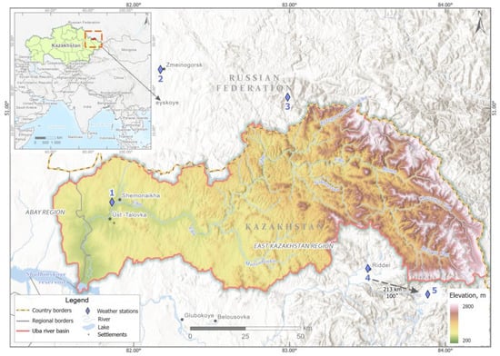
Figure 1.
Geographical location of the Uba River basin and the weather stations whose data were used in this work (weather stations: 1—Shemonaikha, 2—Zmeinogorsk, 3—Babiy Klyuch, 4—Ridder, and 5—Kara-Tyurek).
The stated aims were achieved in several stages: (a) mapping the position of the seasonal snow line during the spring/summer period based on satellite images; (b) determining the melting temperature coefficient of snow cover using meteorological data from the Zmeinogorsk, Shemonaikha, and Ridder stations; (c) performing linear interpolation of mean daily air temperatures for different elevations within the basin and calculating positive temperature sums for specific dates using data from the Shemonaikha, Ridder, Kara-Tyurek, and Babiy Klyuch (Tigirek Nature Reserve) meteorological stations; (d) estimating maximum snow-water equivalent at different elevations using the temperature-based melt-index method and creating maps of maximum snow-water equivalent; (e) analyzing the spatial distribution of maximum snow-water equivalent within the study basin.
The main source of remote sensing information in this study is Sentinel satellite imagery (Figure 2). The Sentinel-2 satellite is part of the Copernicus Earth observation program of the European Space Agency (ESA) [68]. The data were obtained from the official repository of the Copernicus Data Space Ecosystem [69]. The dense set of cloudless or low-cloud images was selected to identify the snow line dynamics more accurately, ensuring coverage of the entire territory of the basin. In total, 204 scenes were processed for four snowmelt periods: 2020—april_12, april_22, may_09, may_14, may_24, may_29, june_23, jul_18; 2021—april_12, april_14, may_02, may_04, may_09, may_29, june_06, june_16, june_18, july_03; 2022—april_12, april_17, april_29, may_09, may_24, june_08, june_23; 2023—april_02, april_22, may_07, may_22, june_01, june_13, june_18, july_03, july_13.
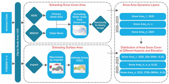
Figure 2.
Flowchart illustrating the proposed creation of snow-cover distribution maps.
Relief data at a 30 m resolution were obtained based on the global digital elevation model, FABDEM (Forest And Buildings removed Copernicus DEM) [70]. The slope aspect data were also derived from FABDEM and then reclassified into two categories: shadow (northern—from 0° to 90° and from 270° to 360°) and light (southern—from 90° to 270°). All image-processing operations and GIS analyses were carried out in the ESRI ArcGIS Pro 3.3.
For automated mapping of snow cover in the study area, the Normalized Difference Snow Index (NDSI) was used [71,72,73]. The NDSI is based on differences in light absorption in the shortwave infrared (SWIR) and visible green (Green) zones of the electromagnetic spectrum (Equation (1)):
where Green is the reflection in the green spectrum, and SWIR1 is the reflection in the shortwave infrared spectrum. After the index was calculated, the data were generalized using a majority filter with a threshold of three pixels to minimize errors along contour boundaries.
NDSI = (Green − SWIR1)/(Green + SWIR1)
The NDSI is widely used in modern research for mapping snow and ice cover, as well as for studying various types of cloud cover over non-snow-covered areas [74,75,76,77,78,79,80,81,82,83,84,85,86,87,88,89]. Using the NDSI significantly reduces the influence of atmospheric effects [90,91,92,93,94,95]. Although various modifications of the NDSI exist—such as the ANDSI (Adjusted Normalized Difference Snow Index), NDFSI (Normalized Difference Forest Snow Index [77]), and NDPCSI (Normalized Difference Principal Component Snow Index)—the classical NDSI approach proved sufficient for accuracy and the relative speed of data acquisition in identifying snow-covered areas.
To calculate the sums of mean daily air temperatures for specific elevations in the Uba River basin, data were used from the Shemonaikha and Ridder meteorological stations and the automatic weather stations of the Tigirek Reserve (Babiy Klyuch) and Kara-Tyurek, located at 320, 740, 1530, and 2601 m above sea level, respectively (Table 1). The mean daily air temperatures were then interpolated across the elevations between the indicated meteorological stations.

Table 1.
Geographical location of meteorological stations, the data of which were used in this work.
To establish the melting temperature coefficient typical for the region, data on mean daily air temperatures, daily precipitation, and the water content of snow cover on routes on specific dates at the Shemonaikha, Zmeinogorsk, and Ridder meteorological stations for 2013–2021 were used. Based on the calculated sums of positive mean daily temperatures on specific dates for specific elevations and the obtained melting coefficient, the maximum snow reserve values for specific elevations were obtained.
Data from ground-based snow measurements conducted by the meteorological service of Kazakhstan from 2020 to 2023 served to verify the calculated values of the snow-cover water reserve.
3. Results and Discussion
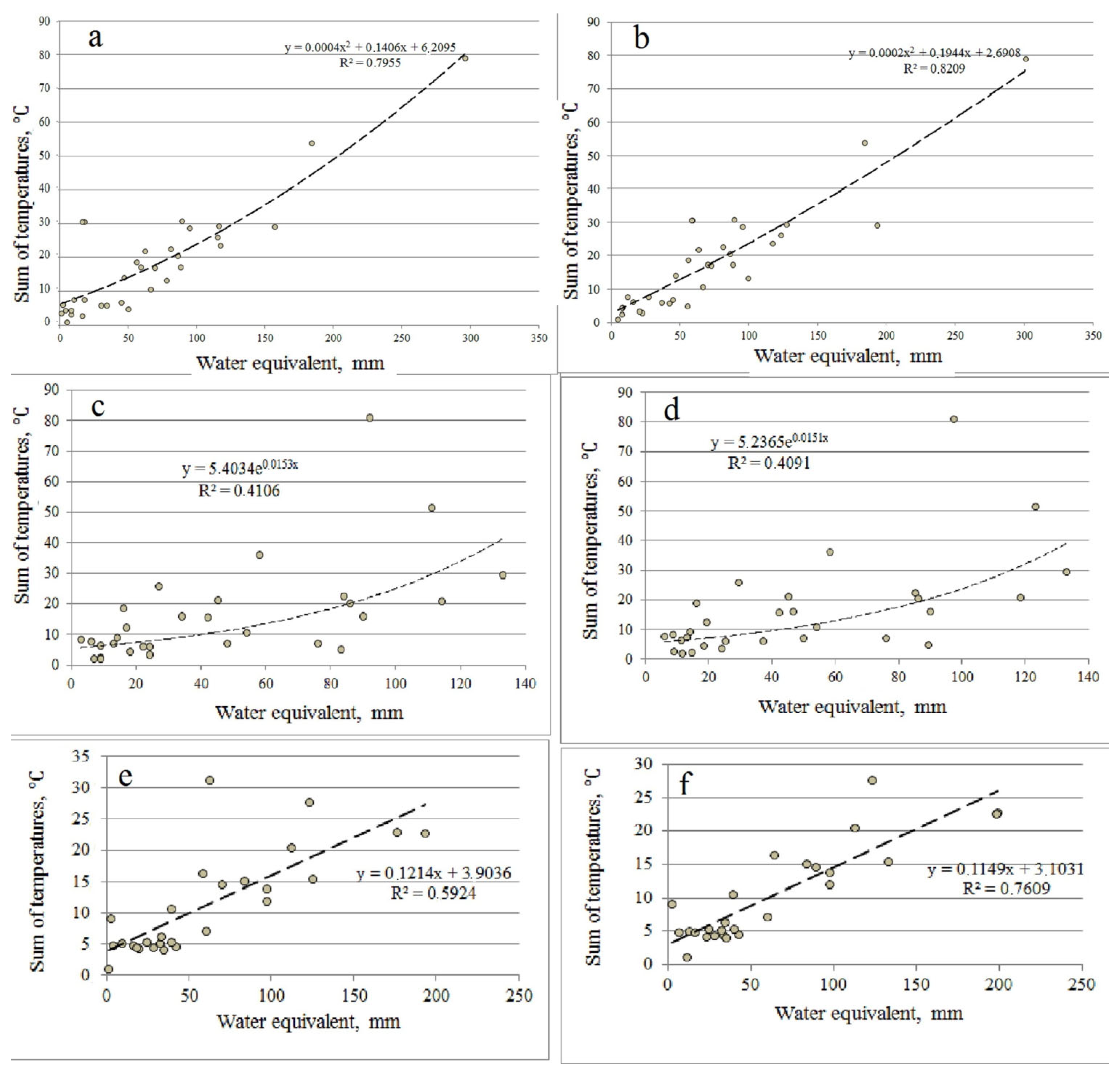
To calculate the melting temperature coefficient of snow cover based on data from the Shemonaikha, Zmeinogorsk, and Ridder meteorological stations, values of snow-water equivalent measured along survey routes, daily atmospheric precipitation, and mean daily air temperatures at a height of 2 m from 2013 to 2022 were used. A total of 34 cases were selected for the Zmeinogorsk station, 30 for the Ridder station, and 27 for the Shemonaikha station (Table 2, Table 3 and Table 4). The highest correlation between the sum of mean daily air temperatures and the snow-cover melt layer during the analyzed periods was observed at the Zmeinogorsk station (correlation coefficient = 0.88). This relationship was weaker at the Shemonaikha and Ridder stations, with correlation coefficients of 0.76 and 0.60, respectively. The correlation between these parameters improved when solid atmospheric precipitation was taken into account for the analyzed periods (Figure 3). However, at the Ridder station, it remained relatively low. The melting temperature coefficient varied widely: from 0.3 to 10.4 mm per degree at the Zmeinogorsk station (Table 2), from 0.4 to 16.6 mm at the Ridder station (Table 3), and from 0.2 to 9.1 mm at the Shemonaikha station (Table 4). However, the average value was 3.7 mm per degree of positive mean daily air temperature at Zmeinogorsk and Ridder, while at Shemonaikha, it was 5.2 mm (Table 2, Table 3 and Table 4).
Table 2.
Snow melting coefficient in water equivalent per degree of positive mean daily air temperature at the Zmeinogorsk weather station for 2013–2021.
Table 3.
Coefficient of snow melting in water equivalent per degree of positive mean daily air temperature at the Ridder weather station for 2013–2022.
Table 4.
Coefficient of snow melting in water equivalent per degree of positive mean daily air temperature at the Shemonaikha weather station for 2013–2021.
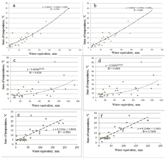
Figure 3.
Dependence of snow-cover melting on the sums of average daily positive air temperatures on snow measurement routes of the Zmeinogorsk (a,b), Ridder (c,d), and Shemonaikha (e,f) meteorological stations for 2013–2021, considering solid atmospheric precipitation (b,d,f) and excluding it (a,c,e).
Considering the precipitation that fell during the period with negative mean daily air temperature, the spread of the values of the melting temperature coefficient values for individual periods remained significant: in Zmeinogorsk—from 1.5 to 11.6 mm (Table 2), in Ridder—from 0.8 to 17.9 mm (Table 3), in Shemonaikha—from 0.2 to 9.8 mm (Table 4). At the same time, its average value in Zmeinogorsk was 4.3 mm per one degree of average daily air temperature; in Ridder, it was 4.1 mm; and in Shemonaikha, it was 5.8 mm. The significant spread of temperature coefficient values between the dates of adjacent snow surveys arose because the processes of heat and moisture exchange between the atmosphere and snow, between snow and soil, and those occurring within the snow layer were not taken into account. Neglecting daytime positive air temperatures on days with negative mean daily values leads to inflated melting coefficients. Observations at the Ridder weather station demonstrated that more accurate inclusion of positive temperatures reduces the melting coefficient by approximately one-quarter. Conversely, low melting coefficients emerge when cold spells between measurement dates cause part of the subsequent heat input to warm the snowpack, rather than melt the snow. The variability in the coefficient decreases when calculations encompass the entire snowmelt period instead of focusing on sequential snow surveys. The average coefficient values also tend to decline with increasing elevation and snow-water equivalent, possibly due to rising air humidity, higher albedo, and greater cloudiness at higher elevations. Ultimately, the value obtained at Ridder was used by the authors to calculate the snow cover’s water reserve at different elevations, primarily because elevations from 400 to 800 m above sea level account for 49% of the Uba River basin’s territory.
The calculation of mean daily air temperature values for different elevations of the study area was possible due to the high similarity of temperature conditions at meteorological stations, the data of which were used in this work: Shemonaikha (Kazakhstan, 320 m), Zmeinogorsk (Russia, 355 m), Ridder (Kazakhstan, 740 m), Babiy Klyuch (Russia, 1530 m), and Kara-Tyurek (Russia, 2601 m). The correlation coefficients between the series of mean daily air temperature values from the lower meteorological stations ranged from 0.96 to 0.99.
The correlation coefficients between the mean daily air temperature series from the upper (Babiy Klyuch, Kara-Tyurek) and lower meteorological stations were also satisfactory. For example, at the Babiy Klyuch–Zmeinogorsk and Babiy Klyuch–Shemonaikha station pairs, these coefficients ranged from 0.82 to 0.95 for individual months of the summer period, making it possible to reconstruct air temperature values during the snowmelt period at different elevations. Temperature correlations between upper and lower meteorological stations were significantly weaker in winter months (Table 5), which can be attributed to winter air temperature inversions. However, this did not affect snowmelt calculations, as melting is rarely observed, even in the lower areas of the study region, before March.
Table 5.
Regression relationship of mean daily air temperatures at the Shemonaikha and Babiy Klyuch meteorological stations for 2013–2021.
Interpolating the average daily air temperature values for different elevations allowed us to calculate and obtain the sums of positive mean daily values for any date (Table 6).
Table 6.
Sums of positive mean daily air temperatures for the Uba River basin in 2021.
To translate the maximum snow-cover water reserve to specific elevations, a melt temperature coefficient of 4.1 mm per degree of positive mean daily air temperature (the average at Ridder) was used, as well as data on the seasonal snow line position obtained from satellite images (Figure 4).
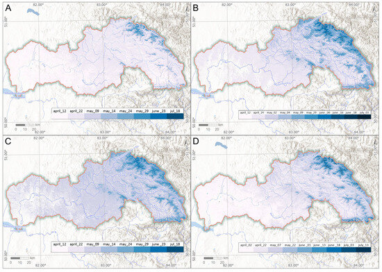
Figure 4.
Position of the seasonal snow line in the Uba River basin in 2020 (A), 2021 (B), 2022 (C), and 2023 (D).
Maps of the seasonal snow line position reflect the diversity of geographical factors influencing snow accumulation. As previously shown [96], major barriers create a so-called “barrier shadow”, leading to minimal snow accumulation on their northern macro-slopes at elevations of 500–1000 m above sea level and earlier snowmelt compared to the same elevations on the southern macro-slopes. However, for smaller-scale barriers, this effect is less pronounced. In such cases, the seasonal snow line on southern slopes is typically about 200 m higher on the same dates. In the watershed areas of mountain ridges, snow cover persists longer on northern slopes due to greater snow-water equivalent formed by both atmospheric precipitation and wind-driven snow transport. As a result, late-summer snow patches, and in some years even perennial snow patches, are observed. Small glaciers still remain near the watersheds of the main barriers, such as the Tigiretsky and Koksuisky ridges.
On the southern slopes of the ridges located 100–200 m below the watersheds, the snow melts early. For example, on the southern macro-slope of the Tigiretsky ridge, snow at elevations of 1700–1900 m melts at the same time as at elevations of 1200–1400 m. However, on barriers with an elevation of 1200 m or less, such a zone of reduced snow accumulation, as well as the earlier melting of the snow cover near watersheds on sunny slopes, is not observed. The greater influx of solar radiation, high wind speeds, and limited snow accumulation near watersheds on the southern slopes result from the fact that the upper forest line on them is approximately 100 m lower than on the northern ones.
High-resolution images make it possible to distinguish many details. They also help detect how terrain slope influences the timing of snow-cover avalanches. Meanwhile, increasing slopes on the southern macro-slope accelerates snow avalanches, whereas on the northern one, it slows it down.
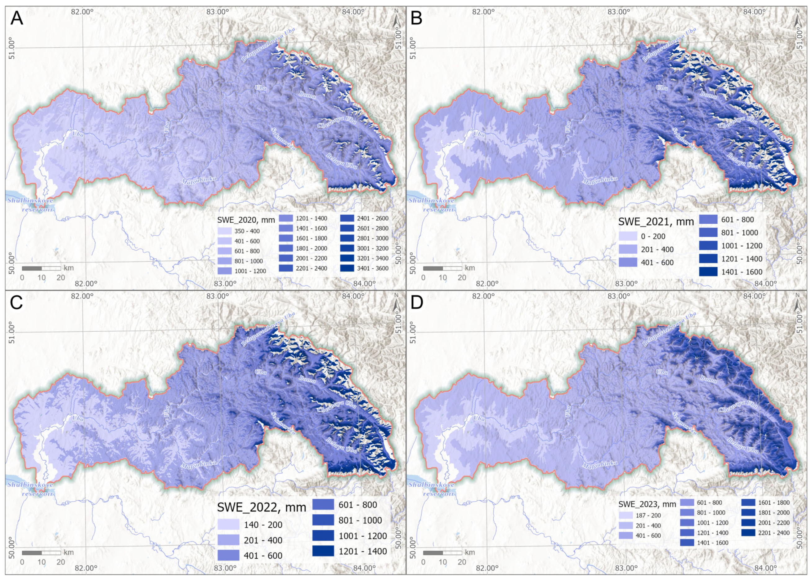
To reduce variation in the differentiation of the snow cover’s water equivalent in constructing a map of maximum snow-water equivalent, the average distribution across shadow and light slopes was calculated. The obtained map confirms the asymmetry in the distribution of snow-water equivalent (Figure 5). At the same elevations, snow-water equivalent is consistently greater on north-facing slopes than on south-facing ones. This pattern is influenced by the prevailing westerly and south-westerly air mass transport and has been theoretically substantiated for the Altai region [97]. However, as shown in our previous research, the situation differs slightly on the western macro-slopes of the Tigiretsky Range, beyond the Uba River basin [96]. Here, up to an elevation of approximately 1200 m above sea level, the snow-water equivalent is greater on the southern macro-slope, whereas at higher elevations, it is greater on the northern macro-slope. The asymmetry in snow distribution reaches its peak near watershed divides. For example, in 2021, field observations on the Tigiretsky Range recorded a maximum snow-water equivalent of 120–125 mm on the southern macro-slope at elevations of 1800–2000 m, while on the northern macro-slope, it exceeded 3000–3700 mm. Despite variations in watershed elevations, the asymmetric snow distribution pattern persists up to approximately 1500 m above sea level. The patchy distribution of snow cover near watershed areas creates diverse ecological niches, each characterized by differences in snow depth, soil freezing, and plant phenophases. For instance, on north-facing slopes, soils remain unfrozen year-round, unlike on south-facing slopes.

Figure 5.
Maximum water reserve of snow cover in the Uba River basin in 2020–2023 (A—2020, B—2021, C—2022, and D—2023).
A comparative analysis of the snow-cover melt layer and water discharge in the Uba River (Figure 6) revealed that, during the high-water (flood) period, daily variation patterns remained synchronized, with peak water discharge lagging by 2–3 days in 2021 and by 1–2 days in 2020. The maximum water discharge in the river was observed when the mean daily air temperature at an elevation of 1000 m reached 10–15 °C. The results obtained align with previously obtained data on the impact of snowmelt on Altai River runoff, especially in the spring season [98,99]. They can be used to predict water discharges and levels during the flood period, thereby reducing risks for society.
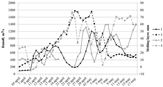
Figure 6.
Water discharge (lines 1,3) at the Uba River (Shemonaikha hydropost) and the daily snow-cover melting layer (water equivalent, lines 2,4) at an elevation of 1000 m above sea level during the spring of 2020 (lines 3,4) and 2021 (lines 1,2).
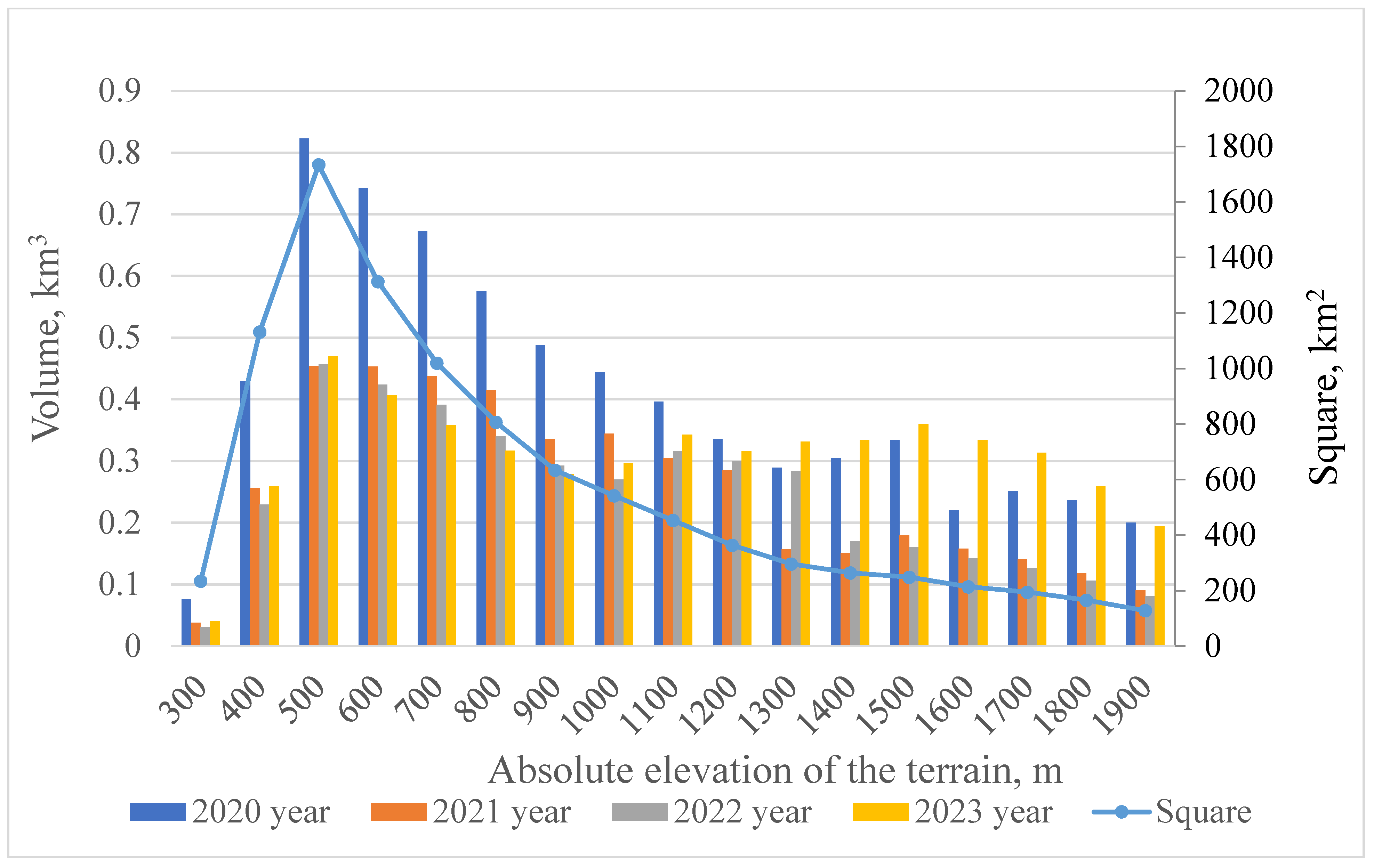
The distribution of water reserves in the snow cover based on elevation ranges in the Uba River basin, though varying from year to year, generally reflects the distribution of areas in the specified ranges (Figure 7). Almost two-thirds of the total snow-cover water reserve of the Uba River basin is concentrated in the elevation range from 400 to 1000 m above sea level. Melting snow at these elevations determines the flood level in the river. Snowmelt at these altitudes determines the flood level in the river. In 2023, the distribution of snow-cover water reserve according to altitude differed somewhat from the distribution in other years in that increased snow accumulation was observed in the altitude range of 1300–1700 m above sea level. This is probably due to the peculiarities of atmospheric circulation in the winter season of this year. However, this issue was not specifically considered in this study. Snowmelt at elevations of approximately 1000 m above sea level determines the flood level in the river. In 2023, the distribution of the snow-cover water reserve according to elevation differed from other years, with enhanced snow accumulation detected at elevations of 1300–1700 m above sea level. Atmospheric circulation patterns during the winter season likely influenced this pattern, although a detailed investigation was not conducted in the present study.

Figure 7.
Distribution of water reserves in snow cover by elevation in the Uba River basin in 2020–2023 and area at elevation levels of the basin.
The values of the snow-cover water reserve derived from calculations were verified using results from ground-based snow measurements carried out by the meteorological service of Kazakhstan between 2020 and 2023 (Table 7). A comparative analysis indicated a close correspondence between the calculated values and observational data. Minor discrepancies may arise from measurement specifics and lack of consideration for brief periods of positive daytime air temperatures. Ground-based observations are generally performed near the anticipated peak of snow accumulation in late March, yet additional snowfall events may shift the maximum accumulation to April. However, in the future, they may increase due to subsequent snowfalls and a shift of the maximum to the month of April.
Table 7.
Snow-cover water reserve established using the temperature-based melt-index (W2) and according to ground-based snow observations (W1).
4. Conclusions
The use of the temperature-based melt-index method makes it possible to determine the maximum snow-water equivalent for the winter period in complex orographic conditions for 2020–2023. This approach helps identify patterns of snow differentiation based on elevation, slope aspect, and distance from watershed divides. Snowmelt coefficients were determined for meteorological stations in Zmeinogorsk, Shemonaikha, and Ridder. This study is the first to quantify the maximum snow-water equivalent in the Uba basin using high-resolution Sentinel-2 imagery and a temperature-index melt model. With no prior basin-scale analyses in the region, the results are genuinely novel. Relative to earlier Altai work, our approach delivers finer spatial detail and independent ground verification, ensuring greater accuracy. By examining aspect- and elevation-controlled contrasts, we provide new insight into snow-cover formation in eastern Kazakhstan and demonstrate the effectiveness of coupling Sentinel-2 data with temperature-index modeling for mountain cryospheric research.
Additionally, this approach improves hydrological modeling, including river discharge and water level forecasts. The data obtained can also be applied to study the impact of snow cover on vegetation structure and dynamics, winter animal migrations, and other ecological processes. In the Uba River basin, in addition to the asymmetric distribution of snow cover according to elevation and slope aspect, divergent trends in maximum snow-water equivalent were observed from 2020 to 2023. Maps illustrating maximum snow-water equivalent and spatial differentiation based on elevation, slope exposure, and watershed proximity were created. In areas closer to the river’s mouth, snow-water equivalent has decreased, while in the headwater region, it has increased. However, the areas occupying the lower reaches of the basin exert the greatest influence on the river’s snow-fed water supply.
Author Contributions
Conceptualization, N.I.B.; methodology, N.I.B. and R.Y.B.; formal analysis, N.I.B., R.Y.B. and A.A.B.; investigation, N.I.B., R.Y.B. and A.A.B.; validation and resources, N.K.Z.; data curation, N.I.B., N.K.Z. and A.D.D.; writing—original draft preparation, N.I.B., R.Y.B. and A.A.B.; writing—review and editing, R.Y.B., A.A.B. and N.K.Z.; visualization, N.I.B. and R.Y.B. All authors have read and agreed to the published version of the manuscript.
Funding
This work was funded by the Science Committee of the Ministry of Science and Higher Education of the Republic of Kazakhstan (Grant Number BR24992899) within the framework of the project “Development of a system for forecasting catastrophic floods in the East Kazakhstan region using remote sensing data, GIS technologies, and machine learning”.
Data Availability Statement
The data that support the findings of this study are not openly available and are available from the corresponding author upon reasonable request.
Conflicts of Interest
The authors declare no conflicts of interest. The funders played no role in the design of the study, in the collection, analyses, or interpretation of data, in the writing of the manuscript, or in the decision to publish the results.
References
- Nefedeva, E.A.; Yashina, A.V. The Role of Snow Cover in Differentiation of the Landscape Sphere; Nauka: Moscow, Russia, 1985; 144p. (In Russian) [Google Scholar]
- Ding, Y.; Mu, C.; Wu, T.; Hu, G.; Zou, D.; Wang, D.; Li, W.; Wu, X. Increasing Cryospheric Hazards in a Warming Climate. Earth-Sci. Rev. 2021, 213, 103500. [Google Scholar] [CrossRef]
- Xu, M.; Sun, Y.; Wang, H.; Qi, P.; Peng, Z.; Wu, Y.; Zhang, G. Altitude Characteristics in the Response of Rain-on-Snow Flood Risk to Future Climate Change in a High-Latitude Water Tower. J. Environ. Manag. 2024, 369, 122292. [Google Scholar] [CrossRef]
- Li, Z.; Cao, Y.; Duan, Y.; Jiang, Z.; Sun, F. Simulation and Prediction of the Impact of Climate Change Scenarios on Runoff of Typical Watersheds in Changbai Mountains, China. Water 2022, 14, 792. [Google Scholar] [CrossRef]
- Velásquez, N.; Quintero, F.; Koya, S.R.; Roy, T.; Mantilla, R. Snow-Detonated Floods: Assessment of the U.S. Midwest March 2019 Event. J. Hydrol. Reg. Stud. 2023, 47, 101387. [Google Scholar] [CrossRef]
- Hao, X.; Huang, G.; Zheng, Z.; Sun, X.; Ji, W.; Zhao, H.; Wang, J.; Li, H.; Wang, X. Development and Validation of a New MODIS Snow-Cover-Extent Product over China. Hydrol. Earth Syst. Sci. 2022, 26, 1937–1952. [Google Scholar] [CrossRef]
- Jiang, L.; Yang, J.; Zhang, C.; Wu, S.; Li, Z.; Dai, L.; Qiu, Y. Daily Snow Water Equivalent Product with SMMR, SSM/I and SSMIS from 1980 to 2020 over China. Big Earth Data 2022, 6, 420–434. [Google Scholar] [CrossRef]
- Zschenderlein, L.; Luojus, K.; Takala, M.; Venäläinen, P.; Pulliainen, J. Evaluation of Passive Microwave Dry Snow Detection Algorithms and Application to SWE Retrieval during Seasonal Snow Accumulation. Remote Sens. Environ. 2023, 288, 113476. [Google Scholar] [CrossRef]
- Mussina, A.; Abdullayeva, A.; Barandun, M.; Cicoira, A.; Tursyngali, M. Assessment of the current state and temporal changes of glacial-moraine lakes in the Central and Eastern part of the northern slope of the Ile Alatau, Kazakhstan. J. Water Land Dev. 2024, 63, 19–24. [Google Scholar] [CrossRef]
- Gul, C.; Kang, S.; Ghauri, B.; Haq, M.; Muhammad, S.; Ali, S. Using Landsat images to monitor changes in the snow-covered area of selected glaciers in northern Pakistan. J. Mt. Sci. 2017, 14, 2013–2027. [Google Scholar] [CrossRef]
- Eker, R.; Bühler, Y.; Schlögl, S.; Stoffel, A.; Aydın, A. Monitoring of Snow Cover Ablation Using Very High Spatial Resolution Remote Sensing Datasets. Remote Sens. 2019, 11, 699. [Google Scholar] [CrossRef]
- Gascoin, S.; Grizonnet, M.; Bouchet, M.; Salgues, G.; Hagolle, O. Theia Snow Collection: High-Resolution Operational Snow Cover Maps from Sentinel-2 and Landsat-8 Data. Earth Syst. Sci. Data 2019, 11, 493–514. [Google Scholar] [CrossRef]
- Bousbaa, M.; Htitiou, A.; Boudhar, A.; Eljabiri, Y.; Elyoussfi, H.; Bouamri, H.; Ouatiki, H.; Chehbouni, A. High-Resolution Monitoring of the Snow Cover on the Moroccan Atlas through the Spatio-Temporal Fusion of Landsat and Sentinel-2 Images. Remote Sens. 2022, 14, 5814. [Google Scholar] [CrossRef]
- Koehler, J.; Bauer, A.; Dietz, A.J.; Kuenzer, C. Towards Forecasting Future Snow Cover Dynamics in the European Alps—The Potential of Long Optical Remote-Sensing Time Series. Remote Sens. 2022, 14, 4461. [Google Scholar] [CrossRef]
- Xiao, X.; Liang, S. Assessment of snow cover mapping algorithms from Landsat surface reflectance data and application to automated snowline delineation. Remote Sens. Environ. 2024, 307, 114163. [Google Scholar] [CrossRef]
- Zhang, Q.; Yuan, Q.; Jin, T.; Song, M.; Sun, F. SGD-SM 2.0: An Improved Seamless Global Daily Soil Moisture Long-Term Dataset from 2002 to 2022. Earth Syst. Sci. Data 2022, 14, 4473–4488. [Google Scholar] [CrossRef]
- Poussin, C.; Peduzzi, P.; Giuliani, G. Snow observation from space: An approach to improving snow cover detection using four decades of Landsat and Sentinel-2 imageries across Switzerland. Sci. Remote Sens. 2025, 11, 100182. [Google Scholar] [CrossRef]
- Snapir, B.; Momblanch, A.; Jain, S.K.; Waine, T.W.; Holman, I.P. A method for monthly mapping of wet and dry snow using Sentinel-1 and MODIS: Application to a Himalayan River basin. Int. J. Appl. Earth Obs. Geoinf. 2019, 74, 222–230. [Google Scholar] [CrossRef]
- Beltramone, G.; Frery, A.C.; German, A.; Bonansea, M.; Scavuzzo, C.M.; Ferral, A. Characterization of Seasonal Snow Covered Surfaces by Sentinel-1 Time Series Anomalies. In Proceedings of the IGARSS 2022–2022 IEEE International Geoscience and Remote Sensing Symposium, Kuala Lumpur, Malaysia, 17–22 July 2022; pp. 1596–1599. [Google Scholar] [CrossRef]
- Kumar, S.; Narayan, A.; Mehta, D.S.; Snehmani. Snow cover characterization using C-band polarimetric SAR in parts of the Himalaya. Adv. Space Res. 2022, 70, 3959–3974. [Google Scholar] [CrossRef]
- Geissler, J.; Rathmann, L.; Weiler, M. Combining daily sensor observations and spatial LiDAR data for mapping snow water equivalent in a sub-alpine forest. Water Resour. Res. 2023, 59, e2023WR034460. [Google Scholar] [CrossRef]
- Torralbo, P.; Pimentel, R.; Polo, M.J.; Notarnicola, C. Characterizing Snow Dynamics in Semi-Arid Mountain Regions with Multitemporal Sentinel-1 Imagery: A Case Study in the Sierra Nevada, Spain. Remote Sens. 2023, 15, 5365. [Google Scholar] [CrossRef]
- Cluzet, B.; Magnusson, J.; Quéno, L.; Mazzotti, G.; Mott, R.; Jonas, T. Exploring how Sentinel-1 wet-snow maps can inform fully distributed physically based snowpack models. Cryosphere 2024, 18, 5753–5767. [Google Scholar] [CrossRef]
- Dunmire, D.; Lievens, H.; Boeykens, L.; De Lannoy, G.J.M. A machine learning approach for estimating snow depth across the European Alps from Sentinel-1 imagery. Remote Sens. Environ. 2024, 314, 114369. [Google Scholar] [CrossRef]
- Deems, J.S.; Painter, T.H.; Finnegan, D.C. Lidar measurement of snow depth: A review. J. Glaciol. 2013, 59, 467–479. [Google Scholar] [CrossRef]
- Dharmadasa, V.; Kinnard, C.; Baraër, M. An Accuracy Assessment of Snow Depth Measurements in Agro-Forested Environments by UAV Lidar. Remote Sens. 2022, 14, 1649. [Google Scholar] [CrossRef]
- Stillinger, T.; Rittger, K.; Raleigh, M.; Michell, A.; Davis, R.; Bair, E. Landsat, MODIS, and VIIRS snow cover mapping algorithm performance as validated by airborne lidar datasets. Cryosphere 2022, 17, 567–590. [Google Scholar] [CrossRef]
- Ackroyd, C.; Donahue, C.P.; Menounos, B.; Skiles, S.M. Airborne lidar intensity correction for mapping snow cover extent and effective grain size in mountainous terrain. GIScience Remote Sens. 2024, 61, 2427326. [Google Scholar] [CrossRef]
- Wendleder, A.; Dietz, A.J.; Schork, K. Mapping Snow Cover Extent Using Optical and SAR Data. In Proceedings of the IGARSS 2018–2018 IEEE International Geoscience and Remote Sensing Symposium, Valencia, Spain, 22–27 July 2018; pp. 5104–5107. [Google Scholar] [CrossRef]
- Hidalgo-Hidalgo, J.-D.; Collados-Lara, A.-J.; Pulido-Velazquez, D.; Fassnacht, S.R.; Husillos, C. Synergistic Potential of Optical and Radar Remote Sensing for Snow Cover Monitoring. Remote Sens. 2024, 16, 3705. [Google Scholar] [CrossRef]
- Wang, H.; Zhang, L.; Wang, L.; He, J.; Luo, H. An Automated Snow Mapper Powered by Machine Learning. Remote Sens. 2021, 13, 4826. [Google Scholar] [CrossRef]
- John, A.; Cannistra, A.F.; Yang, K.; Tan, A.; Shean, D.; Hille Ris Lambers, J.; Cristea, N. High-Resolution Snow-Covered Area Mapping in Forested Mountain Ecosystems Using PlanetScope Imagery. Remote Sens. 2022, 14, 3409. [Google Scholar] [CrossRef]
- Panda, S.; Anilkumar, R.; Balabantaray, B.K.; Chutia, D.; Bharti, R. Machine Learning-Driven Snow Cover Mapping Techniques using Google Earth Engine. In Proceedings of the 2022 IEEE 19th India Council International Conference (INDICON), Kochi, India, 24–26 November 2022; pp. 1–6. [Google Scholar] [CrossRef]
- Adnan, R.M.; Mo, W.; Kisi, O.; Heddam, S.; Al-Janabi, A.M.S.; Zounemat-Kermani, M. Harnessing Deep Learning and Snow Cover Data for Enhanced Runoff Prediction in Snow-Dominated Watersheds. Atmosphere 2024, 15, 1407. [Google Scholar] [CrossRef]
- Mahanthege, S.; Kleiber, W.; Rittger, K.; Rajagopalan, B.; Brodzik, M.J.; Bair, E. A spatially-distributed machine learning approach for fractional snow covered area estimation. Water Resour. Res. 2024, 60, e2023WR036162. [Google Scholar] [CrossRef]
- Hall, D.K.; Salomonson, V.V.; Riggs, G.A. MODIS/Terra Snow Cover 8-Day L3 Global 500 m Grid, version 5; Tile h12v12; National Snow and Ice Data Center: Boulder, CO, USA, 2006. [Google Scholar]
- Wang, X.; Xie, H.; Liang, T. Evaluation of MODIS Snow Cover and Cloud Mask and its Application in Northern Xinjiang, China. Remote Sens. Environ. 2008, 112, 1497–1513. [Google Scholar] [CrossRef]
- Ke, C.Q.; Liu, X. MODIS-observed spatial and temporal variation in snow cover in Xinjiang, China. Clim. Res. 2014, 59, 15–26. [Google Scholar] [CrossRef]
- Marchane, A.; Jarlan, L.; Hanich, L.; Boudhar, A.; Gascoin, S.; Tavernier, A.; Berjamy, B. Assessment of daily MODIS snow cover products to monitor snow cover dynamics over the Moroccan Atlas mountain range. Remote Sens. Environ. 2015, 160, 72–86. [Google Scholar] [CrossRef]
- Riggs, G.A.; Hall, D.K.; Román, M.O. Overview of NASA’s MODIS and Visible Infrared Imaging Radiometer Suite (VIIRS) snow-cover Earth System Data Records. Earth Syst. Sci. Data 2017, 9, 765–777. [Google Scholar] [CrossRef]
- Tran, H.; Nguyen, P.; Ombadi, M.; Hsu, K.-L.; Sorooshian, S.; Qing, X. A cloud-free MODIS snow cover dataset for the contiguous United States from 2000 to 2017. Sci. Data 2019, 6, 180300. [Google Scholar] [CrossRef]
- Zhang, J.; Jia, L.; Menenti, M.; Zhou, J.; Ren, S. Glacier Area and Snow Cover Changes in the Range System Surrounding Tarim from 2000 to 2020 Using Google Earth Engine. Remote Sens. 2021, 13, 5117. [Google Scholar] [CrossRef]
- Calizaya, E.; Laqui, W.; Sardón, S.; Calizaya, F.; Cuentas, O.; Cahuana, J.; Mindani, C.; Huacani, W. Snow Cover Temporal Dynamic Using MODIS Product, and Its Relationship with Precipitation and Temperature in the Tropical Andean Glaciers in the Alto Santa Sub-Basin (Peru). Sustainability 2023, 15, 7610. [Google Scholar] [CrossRef]
- Jin, S.; Sader, S.A. MODIS time-series imagery for forest disturbance detection and quantification. Remote Sens. Environ. 2006, 101, 352–366. [Google Scholar] [CrossRef]
- Wang, Y.; Geerts, B.; Liu, C.; Jing, X. A Convection-Permitting Regional Climate Simulation of Changes in Precipitation and Snowpack in a Warmer Climate over the Interior Western United States. Climate 2025, 13, 46. [Google Scholar] [CrossRef]
- Lavrov, S.A. The Influence of Meteorological Factors, Snow Properties, and Climate Changes on the Snow Cover Melting Processes. Water Sect. Russ. Probl. Technol. Manag. 2024, 1, 46–70. [Google Scholar] [CrossRef]
- Sunita; Sood, V.; Singh, S.; Gupta, P.K.; Gusain, H.S.; Tiwari, R.K.; Khajuria, V.; Singh, D. Estimation and Validation of Snowmelt Runoff Using Degree Day Method in Northwestern Himalayas. Climate 2024, 12, 200. [Google Scholar] [CrossRef]
- Anderson, E.A. Snow Accumulation and Ablation Model–SNOW-17; US National Weather Service: Silver Spring, MD, USA, 2006. Available online: https://www.weather.gov/media/owp/oh/hrl/docs/22snow17.pdf (accessed on 1 February 2025).
- Lee, W.Y.; Gim, H.J.; Park, S.K. Parameterizations of snow cover, snow albedo and snow density in land surface models: A comparative review. Asia-Pac. J. Atmos. Sci. 2024, 60, 185–210. [Google Scholar] [CrossRef]
- Ohmura, A. Physical Basis for the Temperature-Based Melt-Index Method. J. Appl. Meteorol. 2001, 40, 753–761. [Google Scholar] [CrossRef]
- Hock, R. A Distributed Temperature-Index Ice- and Snowmelt Model Including Potential Direct Solar Radiation. J. Glaciol. 1999, 45, 101–111. [Google Scholar] [CrossRef]
- Hock, R. Temperature Index Melt Modelling in Mountain Areas. J. Hydrol. 2003, 282, 104–115. [Google Scholar] [CrossRef]
- Hann, J. Handbuch der Klimatologie (Handbook of Climatology); Verlag von J. Engelhorn: Stuttgart, Germany, 1908; 394p. [Google Scholar]
- Ahlmann, H.W. Le Niveau De Glaciation Comme Fonction De L’accumulation D’humidité Sous Forme Solide: Méthode Pour Le Calcul De L’Humidité Condensée Dans La Haute Montagne Et Pour L’étude De La Fréquence Des Glaciers. Geogr. Ann. 1924, 6, 223–272. [Google Scholar] [CrossRef]
- He, Y.; Chen, C.; Li, B.; Zhang, Z. Prediction of near-surface air temperature in glacier regions using ERA5 data and the random forest regression method. Remote Sens. Appl. Soc. Environ. 2022, 28, 100824. [Google Scholar]
- Turk, F.J.; Miller, S.D. Toward improved characterization of remotely sensed precipitation regimes with MODIS/AMSR-E blended data techniques. IEEE Trans. Geosci. Remote Sens. 2005, 43, 1059–1069. [Google Scholar] [CrossRef]
- Reeh, N. Parameterization of Melt Rate and Surface Temperature on the Greenland Ice Sheet. Polarforschung 1989, 59, 113–128. [Google Scholar]
- Lang, H.; Braun, L. On the Information Content of Air Temperature in the Context of Snow Melt Estimation. In Hydrology of Mountainous Areas; Molnar, L., Ed.; IAHS Press: Wallingford, UK, 1990; pp. 347–354. [Google Scholar]
- Braithwaite, R.J. On Glacier Energy Balance, Ablation, and Air Temperature. J. Glaciol. 1981, 27, 381–391. [Google Scholar] [CrossRef]
- Iglovskaya, N.V.; Narozhny, Y.K. Determination of Snow water equivalent in Altai Using Satellite Information. Bull. Tomsk State Univ. 2010, 334, 160–165. (In Russian) [Google Scholar]
- Gao, L.; Zhang, L.; Shen, Y.; Zhang, Y.; Ai, M.; Zhang, W. Modeling Snow Depth and Snow Water Equivalent Distribution and Variation Characteristics in the Irtysh River Basin, China. Appl. Sci. 2021, 11, 8365. [Google Scholar] [CrossRef]
- Wu, X.; Zhang, W.; Li, H.; Long, Y.; Pan, X.; Shen, Y. Analysis of seasonal snowmelt contribution using a distributed energy balance model for a river basin in the Altai Mountains of northwestern China. Hydrol. Process. 2021, 35, e14046. [Google Scholar] [CrossRef]
- Liu, M.; Xiong, C.; Pan, J.; Wang, T.; Shi, J.; Wang, N. High-resolution reconstruction of the maximum snow water equivalent based on remote sensing data in a mountainous area. Remote Sens. 2020, 12, 460. [Google Scholar] [CrossRef]
- Egorina, A.V. Barrier Factor in the Formation of the Natural Environment of the City; Publishing House of Altai State University: Barnaul, Russia, 2003; 344p. (In Russian) [Google Scholar]
- Bykov, N.I.; Rygalov, E.V.; Shigimaga, A.A. Dendrochronological Analysis of Coniferous Species in Avalanche Catchments of the Northwestern Altai (Korgon River Basin). Ice Snow 2024, 64, 81–95. [Google Scholar] [CrossRef]
- Revyakin, V.S.; Kravtsova, V.I. Snow Cover and Avalanches of Altai; Publishing House of Tomsk State University: Tomsk, Russia, 1977; 215p. (In Russian) [Google Scholar]
- Revyakin, V.S. Natural Ice of the Altai-Sayan Mountain Region; Gidrometeoizdat: Leningrad, Russia, 1981; 288p. (In Russian) [Google Scholar]
- European Space Agency. Available online: https://www.esa.int/Applications/Observing_the_Earth/Copernicus/Sentinel-2 (accessed on 2 November 2024).
- Copernicus Data Space Ecosystem. Available online: https://dataspace.copernicus.eu/ (accessed on 1 October 2024).
- Hawker, L.; Uhe, P.; Paulo, L.; Sosa, J.; Savage, J.; Sampson, C.; Neal, J. A 30m Global Map of Elevation with Forests and Buildings Removed. Environ. Res. Lett. 2022, 17, 24016. [Google Scholar] [CrossRef]
- Hall, D.K.; Riggs, G.A. Normalized-Difference Snow Index (NDSI). In Encyclopedia of Snow, Ice and Glaciers; Singh, V.P., Singh, P., Haritashya, U.K., Eds.; Springer: Dordrecht, The Netherlands, 2011. [Google Scholar] [CrossRef]
- Wang, G.; Jiang, L.; Xiong, C.; Zhang, Y. Characterization of NDSI variation: Implications for snow cover mapping. IEEE Transactions on Geoscience and Remote Sensing. 2022, 60, 1–18. [Google Scholar] [CrossRef]
- Hall, D.K.; Riggs, G.A.; Salomonson, V.V. Development of Methods for Mapping Global Snow Cover Using Moderate Resolution Imaging Spectroradiometer Data. Remote Sens. Environ. 1995, 54, 127–140. [Google Scholar] [CrossRef]
- Salomonson, V.V.; Appel, I. Estimating Fractional Snow Cover from MODIS Using the Normalised Difference Snow Index. Remote Sens. Environ. 2004, 89, 351–360. [Google Scholar] [CrossRef]
- Rittger, K.; Painter, T.H.; Dozier, J. Assessment of methods for mapping snow cover from MODIS. Adv. Water Resour. 2013, 51, 367–380. [Google Scholar] [CrossRef]
- Wang, X.Y.; Wang, J.; Jiang, Z.Y.; Li, H.Y.; Hao, X.H. An Effective Method for Snow-Cover Mapping of Dense Coniferous Forests in the Upper Heihe River Basin Using Landsat Operational Land Imager Data. Remote Sens. 2015, 7, 17246–17257. [Google Scholar] [CrossRef]
- Wang, X.; Wang, J.; Che, T.; Huang, X.; Hao, X.; Li, H. Snow Cover Mapping for Complex Mountainous Forested Environments Based on a Multi-Index Technique. IEEE J. Sel. Top. Appl. Earth Obs. Remote Sens. 2018, 11, 1433–1441. [Google Scholar] [CrossRef]
- Gascoin, S.; Barrou Dumont, Z.; Deschamps-Berger, C.; Marti, F.; Salgues, G.; López-Moreno, J.I.; Revuelto, J.; Michon, T.; Schattan, P.; Hagolle, O. Estimating Fractional Snow Cover in Open Terrain from Sentinel-2 Using the Normalized Difference Snow Index. Remote Sens. 2020, 12, 2904. [Google Scholar] [CrossRef]
- Mahmoodzada, A.B.; Varade, D.; Shimada, S. Estimation of Snow Depth in the Hindu Kush Himalayas of Afghanistan during Peak Winter and Early Melt Season. Remote Sens. 2020, 12, 2788. [Google Scholar] [CrossRef]
- Pozhitkov, R.Y.; Tigeev, A.A.; Moskovchenko, D.V. Assessment of dust deposition in snow cover using remote sensing data: A case study of Nizhnevartovsk. Atmos. Ocean. Opt. 2020, 33, 767–773. [Google Scholar] [CrossRef]
- Singh, K.V.; Setia, R.; Sahoo, S.; Prasad, A.; Pateriya, B. Evaluation of NDWI and MNDWI for assessment of waterlogging by integrating digital elevation model and groundwater level. Geocarto Int. 2015, 30, 650–661. [Google Scholar] [CrossRef]
- Jasrotia, A.S.; Kour, R.; Singh, K.K. Effect of shadow on atmospheric and topographic processed NDSI values in Chenab basin, western Himalayas. Cold Reg. Sci. Technol. 2022, 199, 103561. [Google Scholar] [CrossRef]
- Luo, J.; Dong, C.; Lin, K.; Chen, X.; Zhao, L.; Menzel, L. Mapping Snow Cover in Forests Using Optical Remote Sensing, Machine Learning and Time-Lapse Photography. Remote Sens. Environ. 2022, 275, 113017. [Google Scholar] [CrossRef]
- Rajat, S.; Singh, R.; Prakash, C.; Anita, S. Glacier retreat in Himachal from 1994 to 2021 using deep learning. Remote Sens. Appl. Soc. Environ. 2022, 28, 100870. [Google Scholar] [CrossRef]
- Kairatov, D.A.; Omirzhanova, Z.T. Study of the dynamics of glacier and snow cover changes in the Zailiysky Alatau. Issues Sustain. Dev. Soc. 2022, 8, 1135–1145. [Google Scholar]
- Thaler, E.A.; Crumley, R.L.; Bennett, K.E. Estimating snow cover from high-resolution satellite imagery by thresholding blue wavelengths. Remote Sens. Environ. 2023, 285, 113403. [Google Scholar] [CrossRef]
- Gagarin, L.A.; Baishev, N.E.; Melnikov, A.E. Deciphering signs of underground water icing on Sentinel-1 radar images: A case study of the Verkhne-Neryungrinskaya and Samokitskaya icings in Southern Yakutia. Earth’s Cryosphere 2023, 27, 59–71. [Google Scholar] [CrossRef]
- Kauazov, A.M.; Tillakarin, T.A.; Salnikov, V.G.; Polyakova, S.E. Assessment of changes in snow cover area in Kazakhstan from 2000 to 2022. Curr. Probl. Remote Sens. Earth Space 2023, 20, 298–305. [Google Scholar] [CrossRef]
- Notarnicola, C. Snow cover phenology dataset over global mountain regions from 2000 to 2023. Data Brief 2024, 56, 110860. [Google Scholar] [CrossRef] [PubMed]
- Crane, R.G.; Anderson, M.R. Satellite discrimination of snow/cloud surfaces. Int. J. Remote Sens. 1984, 5, 213–223. [Google Scholar] [CrossRef]
- Dozier, J. Remote sensing of snow characteristics in the southern Sierra Nevada. In Large Scale Effects of Seasonal Snow Cover. Proceedings of the Vancouver Symposium, Vancouver, BC, Canada, 9–22 August 1987; IAHS Publ.: Wallingford, UK, 1987; pp. 305–314. [Google Scholar]
- Dozier, J. Spectral Signature of Alpine Snow Cover from the Landsat Thematic Mapper. Remote Sens. Environ. 1989, 28, 9–22. [Google Scholar] [CrossRef]
- Dozier, J.; Marks, D. Snow Mapping and Classification from Landsat Thematic Mapper Data. Ann. Glaciol. 1987, 9, 97–103. [Google Scholar] [CrossRef]
- EOS Normalized Difference Snow Index (NDSI). Available online: https://eos.com/ru/make-an-analysis/ndsi/ (accessed on 30 September 2024).
- Climateengine. Normalized Difference Snow Index (NDSI). Available online: https://support.climateengine.org/article/101-normalized-difference-snow-index-ndsi/ (accessed on 30 September 2024).
- Bykov, N.I.; Birjukov, R.J. Interrelationships between snowpack dynamics and tree growth in the Tigiretsky Ridge (Altai): Implications for ecological responses to climate variability. Acta Biol. Sib. 2024, 10, 1319–1336. [Google Scholar] [CrossRef]
- Galakhov, V.P. Conditions of Formation and Calculation of Maximum Snow water equivalent in the Mountains: (Based on the Results of Research in Altai); Nauka: Novosibirsk, Russia, 2003; 104p. (In Russian) [Google Scholar]
- Galakhov, V.P.; Samoilova, S.Y.; Mardasova, E.V. Estimation of the amount of winter precipitation in mountain basins and their impact on runoff during floods (using the Charysh and Anuy rivers, Altai as an example). Earth’s Cryosphere 2021, 25, 51–62. [Google Scholar] [CrossRef]
- Galakhov, V.P.; Samoilova, S.Y.; Mardasova, E.V. The influence of snow cover formation conditions on the flood runoff of a mountain river (using the Anuy River basin as an example). Bull. Altai Branch Russ. Geogr. Soc. 2020, 1, 24–33. [Google Scholar]


Disclaimer/Publisher’s Note: The statements, opinions and data contained in all publications are solely those of the individual author(s) and contributor(s) and not of MDPI and/or the editor(s). MDPI and/or the editor(s) disclaim responsibility for any injury to people or property resulting from any ideas, methods, instructions or products referred to in the content. |
© 2025 by the authors. Licensee MDPI, Basel, Switzerland. This article is an open access article distributed under the terms and conditions of the Creative Commons Attribution (CC BY) license (https://creativecommons.org/licenses/by/4.0/).