Article

Resolving the Faint Young Sun Paradox and Climate Extremes: A Unified Thermodynamic Closure Theory

Lamont-Doherty Earth Observatory, Columbia University, Palisades, NY 10964, USA
Climate 2025, 13(6), 116; https://doi.org/10.3390/cli13060116
Submission received: 21 April 2025 / Revised: 27 May 2025 / Accepted: 27 May 2025 / Published: 2 June 2025

Abstract

:
Clouds play a central role in regulating incoming solar radiation and outgoing terrestrial emission; hence, they must be internally constrained to prognose Earth’s temperature. At the same time, planetary fluids are inherently turbulent, so the climate state would tend toward maximum entropy production—a generalized second law of thermodynamics. Incorporating these requirements, I have previously formulated an aquaplanet model to demonstrate that intrinsic water properties may strongly lower the climate sensitivity to solar irradiance, thereby resolving the faint young Sun paradox (FYSP). In this paper, I extend the model to include other external forcings and show that sensitivity to the reduced outgoing longwave radiation by the elevated pCO2 can be several times greater, but the global temperature remains capped at ~40 °C by the exponential increase in saturated vapor pressure. I further show that planetary albedo augmented by a tropical supercontinent may cool the climate sufficiently to cause tropical glaciation. And since the glacial edge is marked by above-freezing temperature, it abuts an open, co-zonal ocean, thereby obviating the “Snowball Earth” hypothesis. Our theory thus provides a unified framework for interpreting Earth’s diverse climates, including the FYSP, the warm extremes of the Cambrian and Cretaceous, and the tropical glaciations of the Precambrian.

Graphical Abstract

1. Introduction

Despite the solar constant being ~20% lower during the Archean than today, geological evidence suggests that Earth remained temperate—perhaps even rivaling the modern warmth [1]. Yet if one assumes a fixed albedo at its modern value, simple energy balance at the top of the atmosphere (TOA) would predict a global frozen surface, hence the long-standing faint young Sun paradox (FYSP) [2]. Since clouds dominate the planetary albedo, it has been proposed that reduced cloud cover, in combination with elevated atmospheric CO2, could compensate for the weaker Sun, but climate models incorporating these factors generally fall short in resolving the paradox [3]. Moreover, these approaches are intrinsically flawed: cloud albedo is an internal variable, so its mere prescription in these models reflects a lack of thermodynamic closure, which necessarily limits their prognostic utility.
To correct this non-closure, I invoke the fact that planetary fluids are inherently turbulent, so the generic climate is a macroscopic manifestation of a non-equilibrium thermodynamic (NT) system, hence governed by the principle of maximum entropy production (MEP)—a generalized second law of thermodynamics. Readers are referred to [4,5] for reviews of MEP and its application in climate studies. Although MEP was proposed initially on empirical grounds [6], its physical foundation has steadily strengthened through the years, including its recent connection to the fluctuation theorem [7,8], which has been validated in laboratory experiments [9,10]. Furthermore, both direct numerical simulations [11] and eddy-resolving calculations [12] of horizontal convection have reproduced MEP’s signature prediction—a mid-latitude front [13]—absent from coarse-grained numerical solutions [14]. Given its broad support, MEP may be reasonably posed as a working hypothesis in our thermodynamic closure.
Using this principle, I previously formulated a minimal aquaplanet model [15] to investigate the global surface temperature. Unlike conventional energy-balance models, it entails interactive low and high clouds, which are well known to regulate the incoming solar radiation and outgoing longwave emission, respectively. In a moving atmosphere, MEP amounts to the maximization of surface dissipation [16,17], hence the turbulent wind, which then specifies the surface temperature. Through the model derivation, it is found that this temperature is constrained by intrinsic water properties to remain within several tens of degrees above the triple point—even with solar irradiance varying by ± 3 0% from its present value. The implication is that, so long as there is an ocean [18], Earth would remain habitable. MEP may thus resolve the FYSP without invoking vanishing cloud albedo and/or unrealistically high p C O 2 .
Beyond the FYSP, Earth’s deep-time climate exhibits extreme states—from torrid Cambrian and Cretaceous to the frigid Precambrian tropical glaciations. Given their probable tectonic origin in the high p C O 2 and tropical supercontinents, I have extended [15] to incorporate these external forcings, thus broadening its application to diverse paleoclimates. As a key addition, I have also removed the empirical treatment of the moisture field, hence the longwave (LW) flux that anchors heat balances, thus enhancing the model’s predictive power.
The presentation below follows the journal’s format. In Section 2 (Methodology), I deduce the physical elements of the model and formulate the thermodynamic closure that specifies the surface temperature. In Section 3 (Results), I prognose the deep-time temperature and offer a physical interpretation of the diverse climates. I provide additional discussions in Section 4 and conclude the paper in Section 5.

2. Methodology

2.1. Physical Configuration

I consider a coupled ocean/atmosphere system depicted in Figure 1. The atmosphere consists of a turbulent planetary boundary layer (PBL, zoomed in for illustration) topped by the lifting condensation level (LCL) and a free troposphere capped by the tropopause. The designated levels are the ocean surface (level 0), the anemometer height (level 1), the LCL (level 2), and the tropopause (level 3). The model includes as internal variables low clouds at the LCL and high clouds at the tropopause, a bimodality that is highly discernible in observations: low clouds being the vast stratus in high latitudes and high clouds being the expansive cirrus over the intertropical convergence zone (ITCZ). Besides their observed prominence, I argue that the two cloud types stem from differing sensible/latent forms of the heat carried by convection: since the latent heat is not released below the LCL, the turbulent PBL is fueled solely by the sensible heat flux, which in turn is expended by radiative cooling from the shallow cloud top, as the latter marks the termination of such turbulence; the condensation above the LCL, on the other hand, continually fuels the rising air in the updraft, whose capping by the tropopause causes outflowing moisture manifested in high clouds.
The two cloud types have very different radiative properties [19]. The low clouds, being of high water density, are highly reflective in the short-wave (SW) band and black in the LW band. The high clouds, on the other hand, are transparent in the SW band because of their low water density but remain black in the LW band because they are made of ice crystals. Given these differing radiative properties, I show that MEP would propel low clouds to high latitudes and high clouds to the tropics [20], a segregation that is highly discernible in observations [21] (his Figure 3.21). Given the vastness of low clouds, they have largely shaded the polar lands, so the land albedo is dominated by the tropical land [22], a feature to be invoked later. Given their geneses argued above, both cloud types are thin; hence, their vertical dimension is neglected, so only heat balances at the designated levels need to be considered.

2.2. Thermal Template

To formulate the heat balance, one needs to determine the clear-sky LW flux, which depends on the moisture profile and lapse rate. These are often assumed in radiative transfer calculations [23] but need to be physically constrained for a deductive theory. As discussed in [24], MEP exerts a strong constraint on these properties, which is summarized below for the self-containment of the paper. Since the irreversible entropy production of the atmosphere stems from convection, MEP would maximize the convective flux, hence its counteracting LW cooling. The latter implies maximized moisture content, so both temperature and specific humidity are propelled toward those of the saturated air in the updraft on account of the Clausius–Clapeyron equation with their deviations specified by entropy and heat balances [24]. Such calculations have reproduced the observed temperature and moisture profiles, and particularly relevant to the present study, they may explain why the surface air is near saturation, why the ambient vapor pressure mimics its saturated counterpart [19], and why the lapse rate is moist–adiabatic despite the small area of the updraft.
The above deductions of the moisture profile and moist–adiabatic lapse rate uniquely specify the clear-sky LW fluxes for a given surface temperature. Based on their asymptotic behavior and aligned with radiative transfer calculations, as discussed below (see also [15]), I fashion the following analytical forms for the surface ( F r , 0 ) and tropopause ( F r , 3 ) LW fluxes:
F r , 0 = B 0 e x p ( B 0 3 ) ,
F r , 3 = 0.9   t a n h ( B 0 / 0.9 ) ,
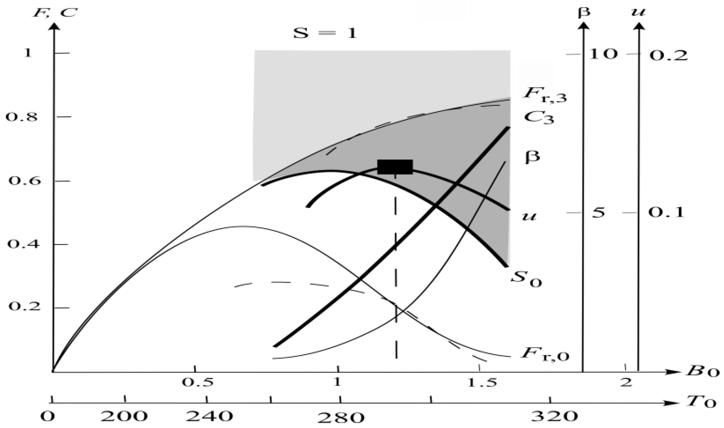
where B 0 is the blackbody radiance of the sea-surface temperature (SST). All heat fluxes have been nondimensionalized by the present solar constant S * = 340   W m 2 , and all symbols, scaling definitions, and parameter values are listed in Appendix A. In our convention, starred variables are dimensional, and numerical subscripts refer to the designated levels. The two LW fluxes (1) and (2) are plotted in Figure 2 (referred to as “climate diagram”) in thin solid lines, together with those from radiative transfer calculations (upper dashed curve from [25] and lower dashed curve from [26]). As the surface warms, both fluxes rise with the blackbody radiance of the surface; the increasing vapor pressure, however, slows the rise in the outgoing LW radiation (OLR) and reverses the surface LW flux, which undergoes an inflection point before it vanishes. Differing from radiative transfer calculations, the analytical forms span the full range of the surface temperature to allow addressing of climate extremes.
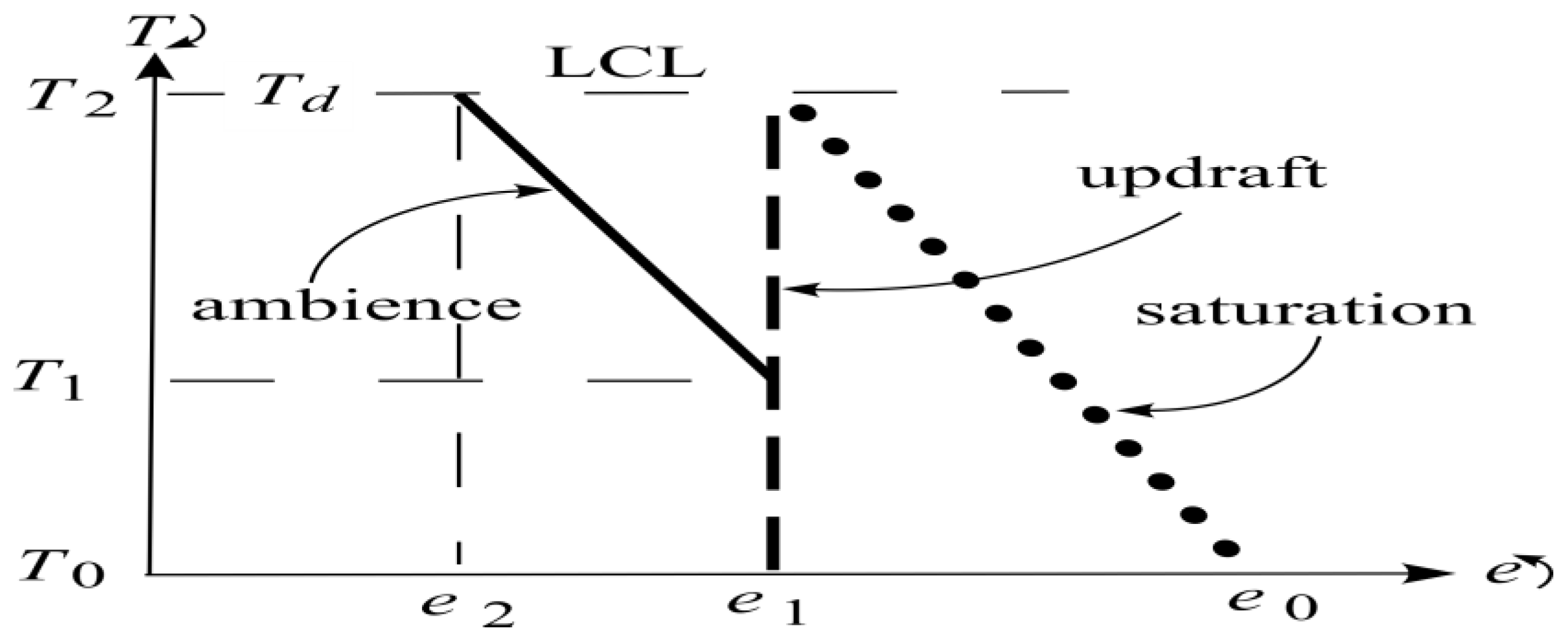
I shall next show that the LCL is sufficiently shallow so that its LW flux can be approximated by that at the surface. For this, we consider the state space of vapor pressure versus temperature (Figure 3) in which the dashed line represents the updraft, the dotted line represents the saturated vapor pressure, and the solid line represents the ambient air (it parallels the saturation line, as discussed earlier). The updraft is initiated when the surface air (of temperature T 1 ) is warmed to the SST ( T 0 ) and rises. The rising air retains the vapor pressure of the ambient air ( e 1 ) and cools off dry–adiabatically until it saturates at the (yet unknown) dew point ( T d ), which defines the LCL. The slope of the saturated vapor pressure e s is given by the Clausius–Clapeyron equation:
d e s d T = L R v e s T 2 ,
where L is the latent heat of evaporation and R v is the gas constant of the water vapor. Integrating this equation yields
e s T = e s , f e x p L R v 1 T f 1 T ,
where e s , f is the saturated vapor pressure at the freezing point ( T f ). Applying this equation to both the surface temperature T 0 and the dew point T d and dividing the resulting two equations and recognizing that the surface relative humidity U is approximately
U = e 1 / e 0 = e s T d / e s ( T 0 ) ,
we derive the dew point
T d = 1 T 0 R v L ln U 1
For a relative humidity of U = 0.7 and a surface temperature varying between 273 and 303 K, the dew point surprisingly varies only between 5 and 6 K below the surface temperature. Since the lapse rate is dry–adiabatic in the updraft, the LCL thus has a height between 0.5 and 0.6 km or an order-of-magnitude shallower than that depicted in Figure 1. In terms of the LW flux, if one takes a LW cooling rate of 1   K / d a y [23], the LW flux at the LCL would be 7   W m 2 greater than the surface one or the latter would be raised by no more than 0.02 in Figure 2, which is assumed negligible.
With the surface air near saturation, the inverse Bowen ratioߞthe ratio of latent to sensible heat fluxes—is approximately ( γ being the Bowen constant):
β 1 γ d e s d T = L γ R v e s T 0 2 ,
which can be calculated from (4) and is drawn in the climate diagram (Figure 2). It can be seen that this ratio increases exponentially as the surface warms. The three thin lines are intrinsic properties of water, which serve as a thermal template in producing varying climates when external forcing changes.

2.3. Heat Balances

In our logical progression, I first consider an aquaplanet and then add the land, p C O 2 and latitude field later. As a first approximation, I neglect the ocean reflectance and spatial correlation between climate variables and forcing, so the global-mean fields (referred to as “global” for short) satisfy
S 0 = S ( 1 r C C 2 ) ,
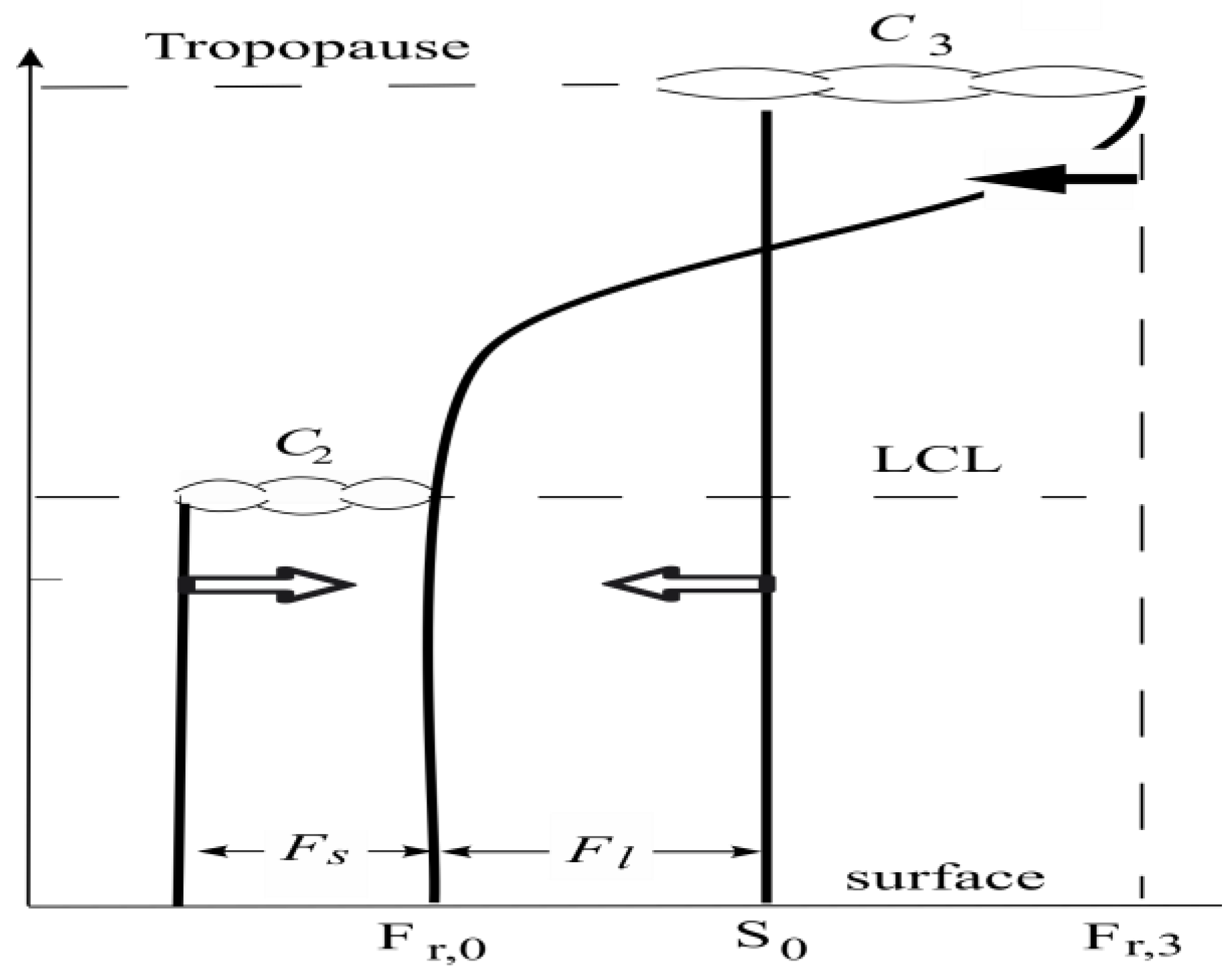
where S 0 is the SW flux absorbed by the ocean (level 0), S is the solar constant, r C is the cloud reflectance, and C 2 is the low-cloud cover (level 2). In the above, S 0 and C 2 are internal variables to be constrained by heat balances, which are sketched in Figure 4.
As seen in this figure, the heat balance at the surface is
S 0 = F s + F l + ( 1 C 2 ) F r , 0 ,
where F s is the sensible heat flux, F l the latent heat flux and F r , 0 the clear-sky LW flux. As discussed in Section 2.1, the low cloud is black and emits at near-surface temperature in the LW band, so it has zeroed out the underlying LW flux. Given the near saturation of the surface air, convective fluxes are linked via
F l = β F s
As discussed in Section 2.1, the sensible heat flux is expended by low-cloud cooling, so the heat balance at the LCL states
S 0 = F l + F r , 0
The above four Equations (8)–(11) form a close set of the four unknowns S 0 ,     C 2 ,     F s , and F l , so they can be solved. Specifically, subtracting (11) from (9) yields
F s = C 2 F r , 0 ,
which restates that the sensible heat flux is expended by cloud-top cooling. It is seen that the low clouds play a dual role in curbing the incoming SW flux by albedo and depleting the sensible heat flux by the LW emission. Substituting C 2 from (8), and combining (10) and (11), we derive the absorbed SW flux
S 0 = F r , 0 ( 1 + β / r C ) 1 + β F r , 0 / ( r C S ) ,
which is plotted in Figure 2 (thick solid line) for the “standard” case of unit forcing. It can be seen that without the latent heat flux (setting β to zero), S 0 is simply the surface LW flux ( F r , 0 ) , and the nonzero latent heat flux has augmented S 0 , which is regulated by cloud albedo, shown in the light shade called “SW cloud forcing”.
With S 0 known, the high cloud is then specified by the TOA heat balance, which states
S 0 = 1 C 3 F r , 3 + C 3 S 0 / 2
where C 3 is the high-cloud cover and F r , 3 , is the clear-sky OLR, noting that because of the vanishing moisture above the tropopause, high clouds are at the skin temperature of blackbody radiance S 0 / 2 [21] (his Equation 3.53). Because of this low emission temperature, the high cloud is highly effective in blocking the OLR to exert a strong greenhouse effect. This low emission temperature, together with the opaque troposphere, on the other hand, has mitigated the high-cloud effect on the surface LW flux, which is neglected. Equation (14) yields a high-cloud cover given by
C 3 = F r , 3 S 0 F r , 3 S 0 / 2 ,
which is plotted in Figure 2 with its warming effect indicated by the dark shade called “LW cloud forcing”. It is seen that global heat balances have coupled the two cloud covers, both of which covary with the surface temperature, but since the dark shade is embedded in the light shade, clouds exert a net cooling, as currently observed [27,28].
Given the differing radiative properties of low and high clouds, their spatial overlap has little effect on the above heat balances: the low cloud does not sense the high cloud since the latter is transparent in the SW band, and its downward LW emission does not reach the LCL; the high cloud on the other hand does not differentiate the low cloud from the surface as they emit at similar temperatures. I shall next link the high-cloud cover to the turbulent wind at the surface.

2.4. Turbulent Wind

As discussed in Section 2.1, the high cloud is a manifestation of the outflowing moisture from the deep updraft as it impinges on the tropopause, and since the outflowing air is supersaturated with respect to ice [29] (their Chapter VIII), the high cloud is dissipated only through the gravitational fallout of ice crystals. As such, it is subject to the water balance of
w i ρ i C 3 = V ρ i m
where w i is the settling velocity of ice crystals, ρ i the ice density, and V the volume flux of the deep updraft. Since there is no condensation below the LCL, the moisture balance of the PBL states that the moisture flux exiting its top equals the surface evaporation or
V e 1 e 2 = C d u * ( e 0 e 1 ) m
where C d is the drag coefficient and u * is the turbulent wind at the surface. Since the ambient vapor pressure parallels the saturation curve and the lapse rate is moist–adiabatic (Section 2.2 and Figure 3), we derive
C d u * V = e 1 e 2 e 0 e 1 = T 1 T 2 T 0 T 2 = γ m γ d m
where γ m and γ d are moist– and dry–adiabatic lapse rates, respectively. And since the moist–adiabatic lapse rate amounts to homogenization of the saturated moist static energy
E s c p T + g z + L q s m
where q s is the saturated specific humidity, we take its vertical derivative and set it to zero to yield
γ m γ d = ( 1 + L c p d q s d T ) 1 ( 1 + 1 γ d e s d T ) 1 1 + β 1
Substituting (16) and (20) into (18) and scaling u * = w i / C d , we derive a simple expression linking the turbulent wind to the high cloud cover
u = C 3 / ( 1 + β ) ,
as plotted in Figure 2. It can be seen that the turbulent wind exhibits a distinct maximum (solid rectangle), which thus specifies the surface temperature in accordance with MEP. The methodology of the study is simply to repeat the above computation of the climate diagram for varying forcing and select the surface temperature at which the turbulent wind peaks, as discussed below.

3. Results

In the climate diagram shown in Figure 2, thin lines represent the thermal template intrinsic to the water, which consists of clear-sky LW fluxes at the surface ( F r , 0 ) and tropopause ( F r , 3 ) as well as the inverse Bowen ratio ( β ). Thick lines are the internal climate variables derived above for the standard case S = 1 . There is a distinct peak in the turbulent wind (solid rectangle), whose origin is readily discerned: as the surface warms, the increasing downward LW emission would be moderated by increasing cloud albedo (the light shade) to maintain the surface heat balance; this weakening of the absorbed SW flux (S0); would expand the high cloud (the dark shade) in maintaining the TOA heat balance; the expanded high cloud implies greater surface evaporation (21), which would first strengthen the turbulent wind but then it would be weakened by the exponential in-crease of the saturated vapor pressure (hence the inverse Bowen ratio β ), resulting in a peak that signifies the MEP (Section 1).
With the above, I have identified a robust mechanism for specifying the surface temperature via MEP, which can be crudely ascribed to the countering effects of greenhouse warming and evaporative cooling, both of which are intrinsic properties of water. I shall next examine its quantitative prediction of the surface temperature to see if it may address the FYSP and climate extremes, as discussed sequentially below under separate headings.

3.1. FYSP

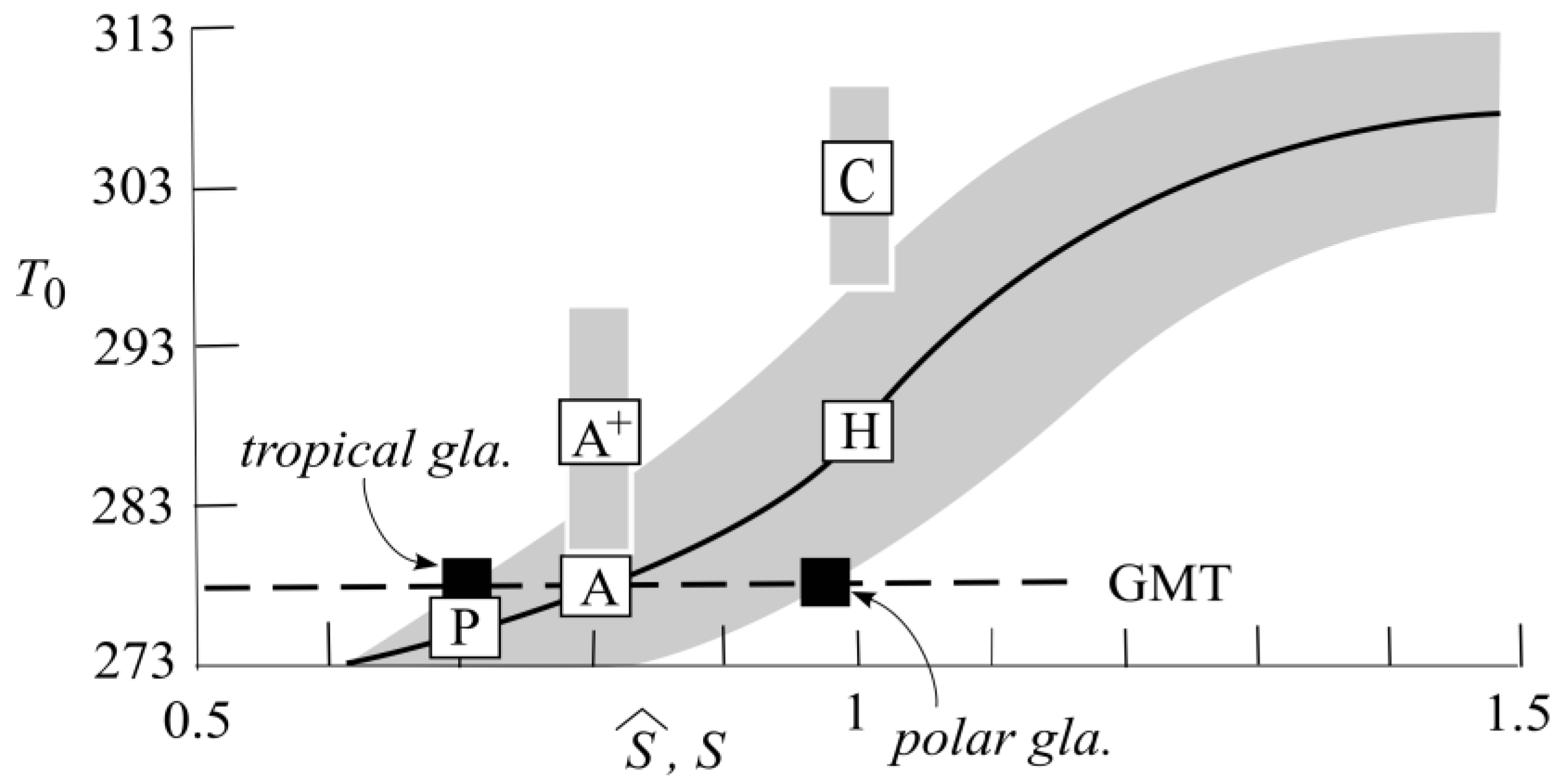
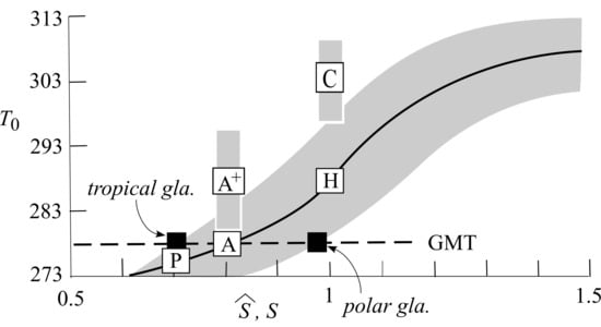
From repeated computations of the climate diagram like Figure 2 for varying forcing, I produce in Figure 5 the MEP-induced surface temperature (solid line) as well as its tropical/polar range (shaded) to be discussed later. The solar forcing spans ± 50 % from the present solar constant, sufficient to address climate extremes. The boxed letters are as follows: H for Holocene, C for Cambrian/Cretaceous, A for Archean, A + for Archean with high p C O 2 , and P for Precambrian with tropical supercontinents. It is seen that climate sensitivity to solar forcing is highly heterogeneous, with a maximum (the inflection point) around the present forcing.
As discussed in Section 2.1, polar lands are mostly shaded by low clouds, so the land albedo is dominated by the tropical land [22]. For the Holocene, I set the tropical land area L 0 = 0.15 and the land reflectance r L = 0.2 to render a land albedo of 0.03 [30], so its solar forcing is 0.97. As such, its climate is approximately that of the standard case shown in Figure 2, which has prognosed a surface temperature of 288 K, just as observed. The deduced cloud albedo is 0.41, which is reasonable for our crude model. This observational test provides valid support for MEP as it differs from energy-balance models that tune the cloud albedo to reproduce the observed temperature, which offers no causal explanation of either, as further underscored below in the context of the FYSP.
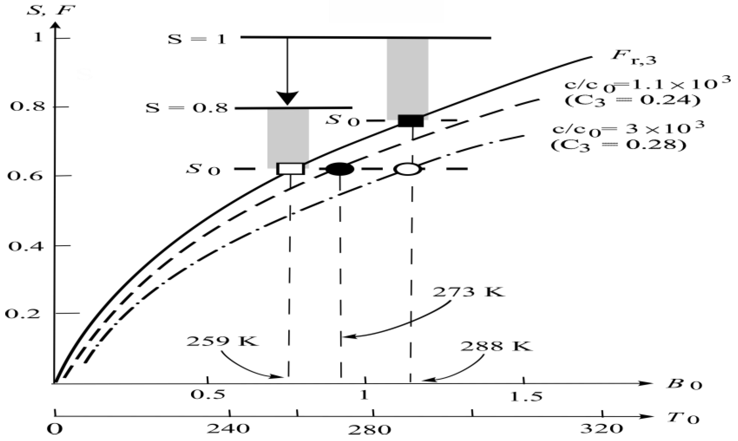
The FYSP pertains to the Archean climate when the Sun is 20–30% dimmer than the present, yet Earth remains habitable, in conflict with that predicted from energy-balance models with the current albedo [2]. The basic argument is as illustrated in Figure 6, wherein horizontal solid and dashed lines are the solar forcing (S) and absorbed SW flux ( S 0 ), respectively, which are spanned by the cloud albedo (shaded column). For the present forcing ( S = 1 ), the cloud albedo is tuned so that S 0 intersects the OLR ( F r , 3 ) at the present temperature of 288 K (solid rectangle), which yields a cloud albedo of 0.23. With this albedo fixed, one may then determine the surface temperature when the Sun is dimmer. Since the Archean land area is smaller than the present [31], we take S = 0.8 to be representative of the solar forcing, which is seen to yield a surface temperature of 259 K (open rectangle), hence a global frozen surface.
It can be easily seen in Figure 6 that if the cloud albedo were to vanish in the Archean, it would be warmer than today. While there is no reason for such an occurrence, it is equally hypothetical to assume that cloud albedo should remain unchanged. Unsure how to constrain the cloud, pre-vious attempts have focused on high pCO2, which would bend the OLR curve to raise the surface temperature. For crude estimates, I apply the formula of [32] (their Table 3) and the current clear-sky OLR ( F r , 3 = 260   W m 2 ) to yield the fractional reduction of the OLR:
δ F r , 3 / F r , 3 = 5.35   l n c / c 0 / 260 = 0.02   l n c / c 0
where c is the pCO2 and subscripted 0 for its present value. The thick dashed and dash-dotted lines are for c / c 0 = 1.1 × 10 3 and 3 × 10 3 , which would raise the surface temperature to 273 K (solid oval) and 288 K (open oval), respectively. As such, the required pCO2 is three orders of magnitude higher than the present, a level that is commensurate with the previously surmised but likely unobserved [2,18]. It is noted that even if such high pCO2 may be approached, it has nonetheless dropped to the present level through the Proterozoic [33], yet Earth remains habitable. To further muddle the problem, the two bent OLR curves correspond to high-cloud cover ( C 3 ) of 0.24 and 0.28, respectively, easily attainable at present [21] (his Figure 3.21). These estimates underscore critical roles played by low/high clouds on the energy entering/leaving the climate system, which thus must be internally constrained in assessing the FYSP—therein lies the fundamental difference of our energy-balance model from the conventional ones.
The solid line of Figure 5 is the MEP solution without the greenhouse effect of pCO2, so the Archean climate with a 20% dimmer Sun is as marked by box A. It shows that the surface temperature is 278 K—well above the freezing point, so there is no FYSP; and the reason is that the dimmer Sun is countered by self-adjusting clouds, which have reduced the climate sensitivity by threefold from 0.43 to 0.15 K / ( W m 2 ) . I reckon, therefore, that the FYSP is an artifact of fixed cloud covers, which has no physical basis.
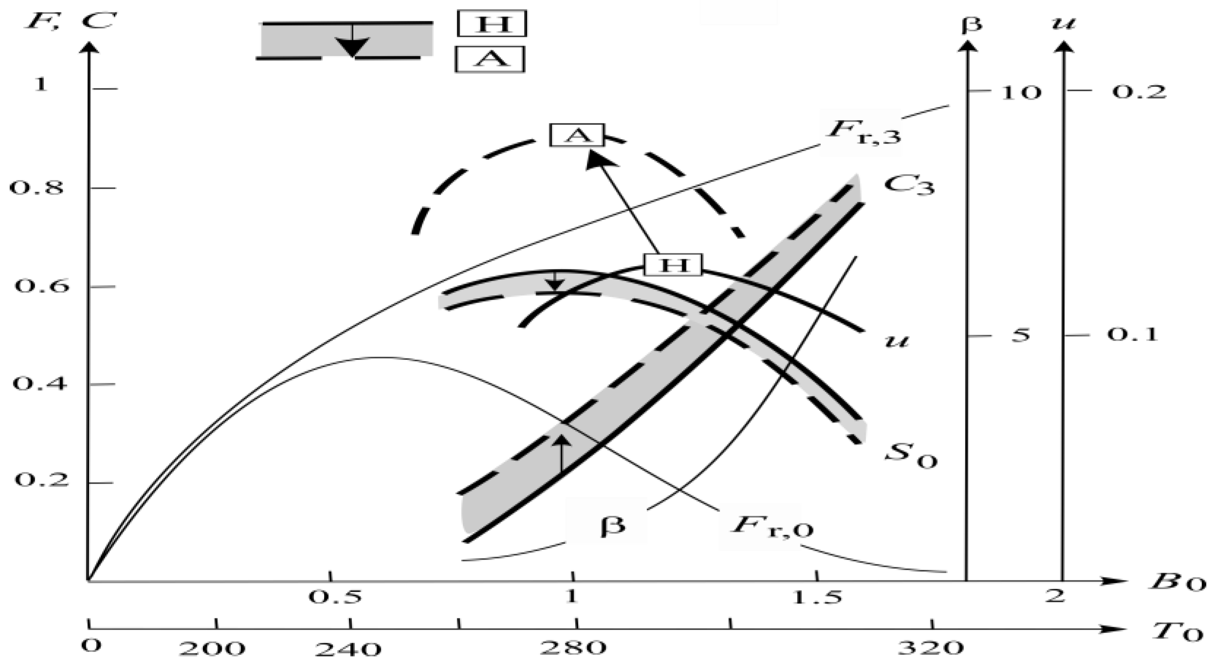
To further elucidate the role of clouds, I show in Figure 7 the change in climate variables from Holocene to Archean (H → A, thick solid to dashed lines). The weaker forcing naturally lowers the absorbed SW flux ( S 0 ), but only slightly because of the moderation by the cloud albedo. This can also be seen from the open arrows of Figure 2: as S 0 decreases, it squeezes the latent ( q l ) (11), hence the sensible ( q s ) (10) heat fluxes, which then shrinks the low cloud ( C 2 ) (12) to counter the decreasing S 0 . It is thus the negative feedback of the cloud albedo that moderates the solar forcing, and its effectiveness stems from the nonlinear—instead of the linear—entry of the solar forcing into (13). The lowered S 0 increases the high-cloud cover (15), hence the turbulent wind (21), but its reduced fractional change against the surface temperature accentuates the effect of increasing β to render a lower surface temperature (boxes H to A).
Although, with MEP, high pCO2 is no longer needed to produce the above-freezing surface temperature, pCO2 is nonetheless observed to be 10–20 times higher than the present in the late Archean when the climate could be as warm as today’s [1]. Can this warmth be accommodated by MEP? For this, I applied the same Formula (22) and c / c 0 = 12 , so clear-sky OLR ( F r , 3 ) would be reduced by 5%, which renders the MEP solution marked by box A + in Figure 5. It has warmed 10 K from box A to 288 K, which thus may explain the temperate climate in the late Archean by the elevated pCO2.
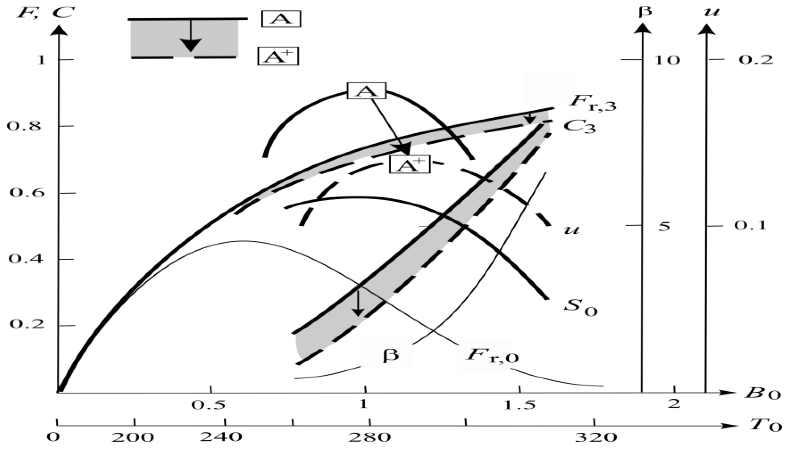
To examine the contrast of A → A+, I plot their climate variables in Figure 8 (thick solid to dashed lines). Since the solar forcing is unchanged, so is the absorbed SW flux ( S 0 ) (13); the reduction in OLR ( F r , 3 ) , however, shrinks the high cloud ( C 3 ) (15), which then pushes the peak of the turbulent wind to a higher temperature (boxes A to A + ), reversing H → A seen in Figure 7. Of particular significance is the magnitude of the reversal: despite OLR reduction of only a small fraction of the solar forcing in H → A, the lack of negative cloud-albedo feedback has produced similar changes (in magnitude) of the high-cloud cover, hence the turbulent wind and temperature. The sensitivity of A → A+ is 0. 81   K / ( W m 2 ) , which is more than five times the sensitivity of H → A.
To recap, given the vast difference in climate sensitivity to the SW and LW forcing, the MEP may resolve both the FYSP when the Sun is dimmer and the late Archean of high p C O 2 that is as warm as today.

3.2. Warm Extreme

Figure 5 shows that the temperature levels off with increasing solar forcing. In such limit ( S ) , the absorbed SW flux (13) becomes
S 0 F r , 0 ( 1 + β / r C )
and the computation of the climate diagram produces a surface temperature of 313 K. The solution obviously needs to be modified when the cloud cover exceeds unity, which can be absorbed into greater cloud reflectance because of the higher water density in a warmer climate. Since this limit is not encountered by the present and colder climate and given the crudeness of the model, such refinements are deemed unwarranted. Since Venus has a solar constant that is about twice the Earth [34], it falls outside our forcing range to conflict with the warm extreme, which is predicated on a global ocean. On the other hand, since the Sun is brightening about 1% every 100 Myr [35], the Earth should remain habitable for another 5 Gyr if the atmospheric composition stays the same.
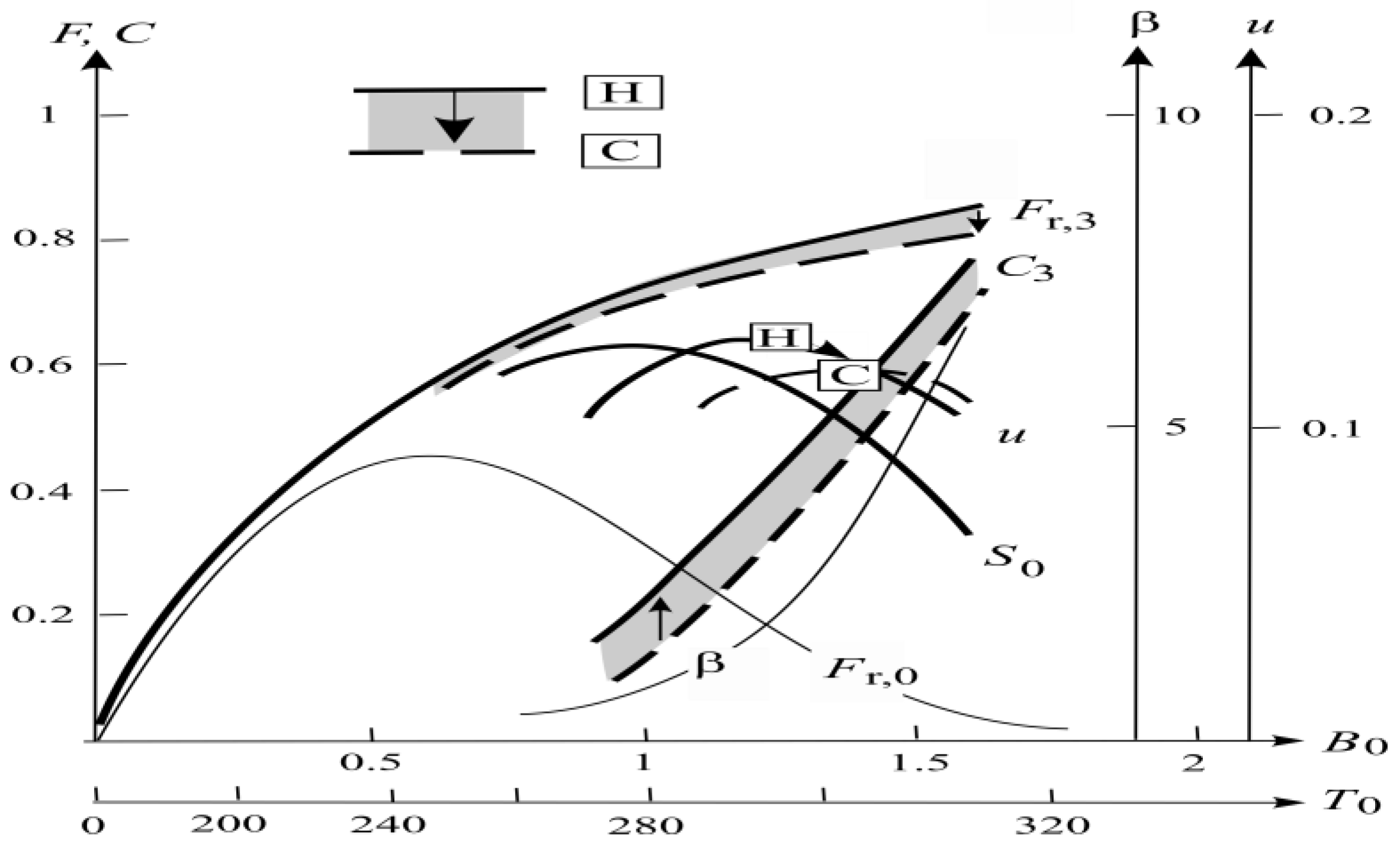
The solar constant has attained the present value in the Paleozoic, but the warmth approaching the warm extreme has occurred in the Cambrian and the Cretaceous; can they be explained by the MEP? For this, we note that both warm periods are accompanied by p C O 2 that is 10–20 times the present value [36], a level that has been reproduced by climate models that have incorporated carbon cycles subject to plausible tectonic conditions, which, however, fall far short of simulating the large swings in the temperature [37]. To see if MEP can remedy this discrepancy, I apply the same Formula (22) with c / c 0 = 12 , which renders the climate of box C (for the Cambrian/Cretaceous) in Figure 5. The contrast of H → C is shown in Figure 9 (from solid to dashed lines), which resembles that of A → A+ (Figure 8), but with a greater warming of 15 K to 303 K. The MEP thus may explain the extreme warmth of the Cambrian/Cretaceous. The sensitivity is 1.2 K / ( W m 2 ) comparable to that of A → A+, which incidentally is similar to that obtained in doubling p C O 2 experiments from climate models [38,39].
Significantly, when we raise the p C O 2 by another ten-fold to one hundred times the present concentration, the temperature remains little changed. Apparently, the exponential growth of β has exerted such a strong constraint that it has curbed further warming of a watery Earth. This deduction from MEP is consistent with the observed Phanerozoic temperature, which fluctuates widely, but all warm episodes seem to be capped by the above asymptote [37], a peculiarity that may now be ascribed to MEP.
One distinct feature of the warm Cretaceous is that its latitudinal temperature range is considerably smaller than the cooler climate [40]. To address this question, I divide the coupled ocean/atmosphere into tropical/polar boxes [8], which shows that their SST difference (referred to as “differential”) is linked linearly to that of the absorbed SW flux, which in turn stems from that of the solar irradiance. The latter depends on Earth’s obliquity hence is largely unchanged since formation of the Moon in the Hadean [41], but it could be altered by differential cloud and land albedos. The cloud albedo, however, is concentrated in high latitudes where the solar irradiance is already low in lessening its impact and then it could be partly compensated by land albedo dominated by the tropical land (recall that the polar sky is mostly overcast, Section 2.1), so as a reasonable approximation, I prescribe the differential absorbed SW flux by the differential solar irradiance ( S * ) , so the differential SST induced by MEP is [42]
T 0 * = S * / α * ,
where α * is the air/sea exchange coefficient
α * = C d ρ a c p u * ( 1 + β ) ,
with C d the drag coefficient, ρ a the surface air density, c p being its specific heat. Nondimensionalized by additional scales [ α * ] = C d ρ a c p u * , T 0 * = S * / [ α * ] , (24) and (25) become
T 0 = 1 / α ,
and
α = u ( 1 + β ) ,
so (21) yields
T 0 = 1 / C 3
Surprisingly, the differential surface temperature is simply the inverse of the high-cloud cover, hence as shaded in Figure 5. Quantitatively, we predict a differential SST of 20 K for the Holocene and 12 K for the Cambrian/Cretaceous, a reduction of about half, consistent with observations [40,43]. The enhanced equitability of the warmer climate is due to the stronger coupling of the ocean/atmosphere (larger α * ), which is a consequence of the Clausius–Clapeyron equation. There is thus no need to invoke changing ocean heat transport [44], which in any event is a part of the climate response and hence may not be independently prescribed. In addition, the deduced covariance of climate equitability with global temperature assures polar amplification—regardless of whether it is global warming or cooling or whether there is sea ice, which thus is a generic property of a watery Earth.

3.3. Cold Extreme

The coldest time on Earth occurred during the Neoproterozoic, when tropical lands were glaciated, leading to the “snowball” hypothesis of a global frozen ocean. This hypothesis, however, has been largely refuted by the sedimentary evidence of an active hydrological cycle that is predicated on an open ocean. Instead, [42] postulated that so long as the tropical continent has highlands above the snowline, it would be glaciated if the summer air temperature (same as the co-zonal SST) falls below the glacial marking temperature (GMT) of ~5 °C. This GMT is drawn in Figure 5 in the dashed line, whose intersections with the differential temperature then set the thresholds for the tropical/polar glaciation.
To include the land albedo in the forcing, we note that MEP has expelled low clouds to high latitudes, thus shading the polar land (Section 2.1). Consequently, the surface albedo is dominated by tropical land, so the absorbed SW flux (8) is altered to
S 0 = S ( 1 r C C 2 r L L 0 ) ,
where r L is the land reflectance and L 0 , the tropical land area. Generalizing the “external” solar forcing to
S ^ = S ( 1 r L L 0 ) ,
it is then represented by the horizonal axis of Figure 5. The solution for the absorbed SW flux (13) is modified to
S 0 = F r , 0 [ 1 + ( β / r C ) S ^ / S ] 1 + β F r , 0 / ( r C S ) ,
while other climate variables retain the original expressions. In addition to the Neoproterozoic, tropical glaciations accompanied most Precambrian supercontinents [45], with the solar constant spanning over the range 0.7–0.9 of its current value [46], so as a representative example, I set S = 0.8 , tropical land area L 0 = 0.3 , and its reflectance r L = 0.4 (before the advent of vascular vegetation) to yield S ^ 0.7 . Although the Neoproterozoic solar constant is near the high end, it is partly offset by the greater land albedo effect on the brighter tropical Sun. The resulting MEP solution is marked by box P (for Precambrian) in Figure 5. Since the tropical temperature has lowered to the GMT, there would be glaciation over the tropical land so long as it is characterized by orogenic highlands above the snow-line [42]. One notes that since the polar land is already glaciated when the solar forcing is slightly lower than the present, as attested by the Pleistocene ice ages, the higher ice reflectance over the cloud reflectance could augment the planetary albedo even under an overcast sky to amplify the global cooling. On the other hand, so long as the global temperature remains above the freezing point, tropical glaciation would coexist with an open co-zonal ocean, a critical feature that is in line with observations but obviates the snowball hypothesis.
There, however, is no physical prohibition to global frozen surface if the solar forcing falls below about 0.6, in which case the shutoff of the absorbed SW flux would vault the Earth to the pre-greenhouse state of extreme coldness. This prognosis is consistent with the frozen Mars as its solar constant is about 0.43 [34]. But since it deviates from the thawed state by only 20% of the Earth’s solar constant, one may not preclude the presence of liquid water in its past if the atmospheric composition was favorable [47]. And then, since the Sun is brightening about 1% every 100 Myr, Mars may become habitable in less than 2 Gyr, possibly before Earth becomes too hot for life.

4. Discussion

While our minimal model is admittedly crude, it benefits from having far fewer tunable parameters than comprehensive climate models. One key uncertainty is cloud reflectance, which is set to 0.5 based on observational evidence [19], replacing the arbitrary unit value used in [15]. TThis adjustment raises the prognosed Holocene temperature from 280 K to 288 K, which represents a substantial improvement in support of MEP. Given the shallow lifting condensation level, SW absorption (b) occurs mainly in the free troposphere, so the upper bracketed term in (13) would be modified to 1 + ( 1 b ) β / r c , justifying its neglect under b 1 . Although spatial correlations are neglected in global balances, the derivation of the latitudinal trend allows them to be absorbed into uncertain reflectances; hence, it does not seriously limit the theory.
A key advance of our theory is its ability to prognose Earth’s temperature with interactive clouds, which provide the internal degrees of freedom that are closed by MEP. Climate models that prescribe or parameterize clouds to reproduce the present condition [3,48,49,50] lack the closure to prognose a vastly different paleoclimate—regardless of their complexity. The authors of [51] advocate 3-D GCMs to capture cloud feedback; our results suggest that it is not the spatial dimensionality but thermodynamic closure that is needed to resolve the FYSP. Although high-cloud feedback to the local temperature has been suggested based on short-term tropical observations [52,53], its relevance to global cover is minimal, which is necessarily coupled with low-cloud cover and global temperature through global heat balance (Section 2.2).
This author [42] has proposed that tropical glaciation could result from the presence of tropical supercontinents, without requiring a global frozen ocean. To account for both the necessary cooling and the extreme warmth of the Cambrian, he invoked the high climate sensitivity derived from pCO2-doubling experiments. The present study reveals however that although sensitivity to pCO2-induced change remains comparable, sensitivity to changing solar irradiance is much lower due to moderation by cloud albedo. As a consequence, these contrasting sensitivities, revealed through the MEP closure, provide a coherent explanation of both the FYSP and the extreme warmth of the Cambrian and Cretaceous.
Although atmospheric pCO2 is strongly coupled to—hence equilibrates with—the global temperature over a million-year timescale [54], tectonically driven changes in pCO2 may nonetheless act as external forcing of the climate system, as demonstrated in climate models incorporating carbon cycles [37]. While these models have reproduced the observed pCO2, they typically fall short in capturing the temperature variation. This discrepancy is now bridged by the elevated sensitivity caused by self-adjusting high clouds.

5. Conclusions

This study presents a minimal climate model aimed at addressing key features of Earth’s deep-time climate, including the faint young Sun paradox (FYSP) and extreme climate states. Departing from traditional energy-balance models, the formulation incorporates freely evolving low and high clouds, which regulate incoming solar and outgoing thermal radiation, respectively. These additional internal degrees of freedom enable thermodynamic closure based on maximum entropy production (MEP), a generalized second law of thermodynamics.
The model predicts that intrinsic water properties would constrain the global sur-face temperature to within several tens of degrees above the triple point—even when the solar constant varies by ±30% relative to its present value. The much-reduced sensitivity to solar forcing is due to the negative feedback of the cloud albedo, which thus may possibly resolve the FYSP.
In contrast, the model shows that sensitivity to pCO2-induced reduction in outgoing longwave radiation, which lacks direct moderation by cloud albedo, can be several times larger. Nonetheless, the surface temperature remains capped at ~40 °C due to the exponential rise in the saturated vapor pressure with temperature—a prediction that is consistent with the observed warmth of the Cambrian and Cretaceous.
The dimmer Precambrian Sun combined with tropical supercontinents unsheltered by high-latitude low clouds may cool the tropical land to below the glacial threshold of ~5 °C to cause tropical glaciation. Crucially, since this threshold is above the freezing point, the glacial edge would abut an open co-zonal ocean, thus obviating the “snowball Earth” hypothesis.
In conclusion, allowing low and high clouds as internal variables of the climate system has exposed vastly different climate sensitivities to SW and LW forcings, through which our theory may provide a unified thermodynamic framework for understanding the FYSP and warm/cold extremes of the Earth’s deep-time climate.

Funding

This research received no external funding.

Data Availability Statement

No new data were created or analyzed in this study. Data sharing is not applicable since the article describes entirely theoretical research.

Acknowledgments

I want to thank the anonymous reviewers for their comments that helped to improve the paper.

Conflicts of Interest

The author declares no conflicts of interest.

Appendix A. Symbols

AArchean climate
A+Archean climate with high pCO2
bSW absorption
B0Surface blackbody radiance
cpCO2
c 0 Present pCO2
c p Specific heat of surface air (=103 J kg−1K−1)
C Cambrian/Cretaceous climate
C d Drag coefficient (=10−3)
C 2 Low-cloud cover
C 3 High-cloud cover
eWater vapor pressure
e s Saturated vapor pressure
e s , f Saturated vapor pressure at freezing point (=6.11 mb)
E s Saturated moist static energy
F s Sensible heat flux
F l Latent heat flux
F r , 0 Surface LW flux
F r , 3 Tropopause LW flux
HHolocene climate
L Latent heat of evaporation (=2.26 × 10⁶ J kg−1)
L 0 Tropical land area
P Precambrian climate with tropical supercontinent
pCO2Partial pressure of atmospheric CO2
q s Saturated specific humidity
r C Cloud reflectance (=0.5)
r L Land reflectance
R v Gas constant of water vapor ( = 461   J   K 1 k g 1 )
S * Present solar constant ( = 340   W   m 2 )
S * Differential solar irradiance ( = 150   W   m 2 )
SSolar constant
S ^ Solar forcing
S 0 Absorbed SW flux
T Temperature
T d Dew point
T f Freezing point
T 0 * Differential SST
[ T 0 * ] Scale of T 0 * ( = S * / [ α * ] = 7.5   K )
U   Surface relative humidity ( = 0.7 )
u * Surface turbulent wind
[ u * ] Scale of u * ( = w i / C d = 20   m   s 1 )
V Updraft volume flux
w i Settling velocity of ice crystals ( = 2   c m   s 1 )
α * Air-sea exchange coefficient
[ α * ] Scale of α * ( = 20   W   m 2   K 1 )
β Saturated inverse Bowen ratio
γ Bowen constant ( = 0.61   m b   K 1 )
γ d Dry–adiabatic lapse rate ( = 10   K   k m 1 )
γ m Moist–adiabatic lapse rate
ρ a Surface air density ( = 1   k g   m 3 )
ρ i Ice density

References

  1. Blake, R.E.; Chang, S.J.; Lapland, A. Phosphate oxygen isotopic evidence for a temperate and biologically active Archaean ocean. Nature 2010, 464, 1029–1032. [Google Scholar] [CrossRef] [PubMed]
  2. Kasting, J.F. Faint young Sun redux. Nature 2010, 464, 687–689. [Google Scholar] [CrossRef]
  3. Goldblatt, C.; Zahnle, K.J. Clouds and the faint young Sun paradox. Clim. Past 2011, 7, 203–220. [Google Scholar] [CrossRef]
  4. Ozawa, H.; Ohmura, A.; Lorenz, R.D.; Pujol, T. The second law of thermodynamics and the global climate system: A review of the maximum entropy production principle. Rev. Geophys. 2003, 41, 10182003. [Google Scholar] [CrossRef]
  5. Kleidon, A. Non-equilibrium thermodynamics and maximum entropy production in the Earth system: Applications and implications. Naturwissenschaften 2009, 96, 653–677. [Google Scholar] [CrossRef] [PubMed]
  6. Paltridge, G. Global dynamics and climate-a system of minimum entropy exchange. Q. J. R. Meteorol. Soc. 1975, 101, 475–484. [Google Scholar] [CrossRef]
  7. Dewar, R.C. Maximum entropy production and the fluctuation theorem. J. Phys. A Math. Gen. 2005, 38, L371–L381. [Google Scholar] [CrossRef]
  8. Ou, H.W. Thermohaline circulation: A missing equation and its climate change implica-tions. Clim. Dyn. 2018, 50, 641–653. [Google Scholar] [CrossRef]
  9. Evans, D.J.; Searle, D.J. The fluctuation theorem. Adv. Phys. 2002, 51, 1529. [Google Scholar] [CrossRef]
  10. Wang, G.M.; Sevick, E.M.; Mittag, E.; Searles, D.J.; Evans, D.J. Experimental demonstration of violations of the Second Law of Thermodynamics for small systems and short time scales. Phys. Rev. Lett. 2002, 89, 050601/1–050601/4. [Google Scholar] [CrossRef]
  11. Hogg, A.M.; Gayen, B. Ocean gyres driven by surface buoyancy forcing. Geophys. Res. Lett. 2020, 47, e2020GL088539. [Google Scholar] [CrossRef]
  12. Liu, T.; Ou, H.W.; Liu, X.; Chen, D. On the role of eddy mixing in the subtropical ocean circulation. Front. Mar. Sci. 2022, 9, 832992. [Google Scholar] [CrossRef]
  13. Ou, H.W. Meridional thermal field of a coupled ocean-atmosphere system: A conceptual model. Tellus 2006, 58A, 404–415. [Google Scholar] [CrossRef]
  14. Colin de Verdière, A. Buoyancy driven planetary flows. J. Mar. Res. 1988, 46, 215–265. [Google Scholar] [CrossRef]
  15. Ou, H.W. Possible bounds on the earth’s surface temperature: From the perspective of a conceptual global-mean model. J. Clim. 2001, 14, 2976–2988. [Google Scholar] [CrossRef]
  16. Lorenz, E.N. Generation of available potential energy and the intensity of the general circulation. In Climate Dynamics; Pfeffer, R.C., Ed.; Pergamon Press: Oxford, UK, 1960; pp. 86–92. [Google Scholar] [CrossRef]
  17. Kleidon, A. Working at the limit: A review of thermodynamics and optimality of the Earth system. Earth Syst. Dyn. 2023, 14, 861–896. [Google Scholar] [CrossRef]
  18. Feulner, G. The faint young Sun problem. Rev. Geophys. 2012, 50, RG2006. [Google Scholar] [CrossRef]
  19. Webster, P.J. The role of hydrological processes in ocean-atmosphere interactions. Rev. Geophys. 1994, 32, 427–476. [Google Scholar] [CrossRef]
  20. Ou, H.W. Hemispheric symmetry of planetary albedo: A corollary of nonequilibrium thermodynamics. Atmos 2023, 14, 1243. [Google Scholar] [CrossRef]
  21. Hartmann, D.L. Global Physical Climatology; Academic Press: New York, NY, USA, 1994; p. 411. [Google Scholar]
  22. Barron, E.J.; Sloan, J.L., II; Harrison, C.G. Potential significance of land-sea distribution and surface albedo variations as a climatic forcing factor: 180 m.y. to the present. Palaeogeogr. Palaeoclimatol. Palaeoecol. 1980, 30, 17–40. [Google Scholar] [CrossRef]
  23. Manabe, S.; Strickler, R.F. Thermal equilibrium of the atmosphere with a convective adjustment. J. Atm. Sci. 1964, 21, 361–385. [Google Scholar] [CrossRef]
  24. Ou, H.W. Hydrological cycle and ocean stratification in a coupled climate system: A theoretical study. Tellus A Dyn. Meteorol. Oceanogr. 2007, 59, 683–694. [Google Scholar] [CrossRef]
  25. Pierrehumbert, R.T. Thermostats, radiator fins, and the local runaway greenhouse. J. Atmos. Sci. 1995, 52, 1784–1806. [Google Scholar] [CrossRef]
  26. Hartmann, D.L.; Michelsen, M.L. Large-scale effects on the regulation of tropical sea surface temperature. J. Clim. 1993, 6, 2049–2062. [Google Scholar] [CrossRef]
  27. Ramanathan, V. The role of earth radiation budget studies in climate and general circulation research. J. Geophys. Res. Atmos 1987, 92, 4075–4095. [Google Scholar] [CrossRef]
  28. Hartmann, D.L.; Doelling, D. On the net radiative effectiveness of clouds. J. Geophys. Res. Atmos 1991, 96, 869–891. [Google Scholar] [CrossRef]
  29. Borovikov, A.M.; Gaivoronskii, I.I.; Zak, E.G.; Kostarev, V.V.; Mazin, I.P.; Minervin, V.E.; Khrgian AK, S.M. Cloud Physics (Translated from Russian); Israel Program for Scientific Translations Ltd.: Jerusalem, Israel, 1963; p. 392. [Google Scholar]
  30. Donohoe, A.; Battisti, D.S. Atmospheric and surface contributions to planetary albedo. J. Clim. 2011, 24, 4402–4418. [Google Scholar] [CrossRef]
  31. Rosing, M.T.; Bird, D.K.; Sleep, N.H.; Bjerrum, C.J. No climate paradox under the faint early Sun. Nature 2010, 464, 744–747. [Google Scholar] [CrossRef] [PubMed]
  32. Myhre, G.; Highwood, E.J.; Shine, K.P.; Stordal, F. New estimates of radiative forcing due to well mixed greenhouse gases. Geophys. Res. Lett. 1998, 25, 2715–2718. [Google Scholar] [CrossRef]
  33. Sheldon, N.D. Precambrian paleosols and atmospheric CO2 levels. Precambrian Res. 2006, 147, 148–155. [Google Scholar] [CrossRef]
  34. NASA (n.d.) Planetary Fact Sheet—Metric. NASA Goddard Space Flight Center, Solar System Exploration Data Services. Available online: https://nssdc.gsfc.nasa.gov/planetary/factsheet/ (accessed on 18 April 2025).
  35. Sackmann, I.; Boothroyd, A.I.; Kraemer, K.E. Our sun III, Present and future. Astrophys. J. 1993, 418, 457. [Google Scholar] [CrossRef]
  36. Berner, R.A.; Kothavala, Z. GEOCARB III: A revised model of atmospheric CO2 over Phanerozoic time. Am. J. Sci. 2001, 301, 182–204. [Google Scholar] [CrossRef]
  37. Mills, B.J.; Krause, A.J.; Scotese, C.R.; Hill, D.J.; Shields, G.A.; Lenton, T.M. Modelling the long-term carbon cycle, atmospheric CO2, and Earth surface temperature from late Neoproterozoic to present day. Gondwana Res. 2019, 67, 172–186. [Google Scholar] [CrossRef]
  38. Hansen, J.E. A slippery slope: How much global warming constitutes “dangerous anthropogenic interference”? Clim. Chang. 2005, 68, 269–279. [Google Scholar] [CrossRef]
  39. Meehl, G.A.; Senior, C.A.; Eyring, V.; Flato, G.; Lamarque, J.F.; Stouffer, R.J.; Taylor, K.E.; Schlund, M. Context for interpreting equilibrium climate sensitivity and transient climate response from the CMIP6 Earth system models. Sci. Adv. 2020, 6, eaba1981. [Google Scholar] [CrossRef] [PubMed]
  40. Barron, E.J. A warm, equable Cretaceous: The nature of the problem. Earth-Sci. Rev. 1983, 19, 305–338. [Google Scholar] [CrossRef]
  41. Laskar, J.; Robutel, P. The chaotic obliquity of the planets. Nature 1993, 361, 608–612. [Google Scholar] [CrossRef]
  42. Ou, H.W. Tropical Glaciation and Glacio-Epochs: Their Tectonic Origin in Paleogeography. Climate 2025, 13, 9. [Google Scholar] [CrossRef]
  43. Hearing, T.W.; Harvey, T.H.; Williams, M.; Leng, M.J.; Lamb, A.L.; Wilby, P.R.; Gabbott, S.E.; Pohl, A.; Donnadieu, Y. An early Cambrian greenhouse climate. Sci. Adv. 2018, 5, eaar5690. [Google Scholar] [CrossRef]
  44. Barron, E.J.; Peterson, W.H.; Pollard, D.; Thompson, S. Past climate and the role of ocean heat transport: Model simulations for the Cretaceous. Paleoceanography 1993, 8, 785–798. [Google Scholar] [CrossRef]
  45. Eyles, N. Glacio-epochs and the supercontinent cycle after∼ 3.0 Ga: Tectonic boundary conditions for glaciation. Palaeogeogr. Palaeoclim. Palaeoecol. 2008, 258, 89–129. [Google Scholar] [CrossRef]
  46. Bahcall, J.N.; Pinsonneault, M.H.; Basu, S. Solar models: Current epoch and time dependences, neutrinos, and helioseismological properties. Astrophys. J. 2001, 10, 990. [Google Scholar] [CrossRef]
  47. Haberle, R.M.; McKay, C.P.; Schaeffer, J.; Cabrol, N.A.; Grin, E.A.; Zent, A.P.; Quinn, R. On the possibility of liquid water on present-day Mars. J. Geophys. Res. Planets 2001, 106, 23317–23326. [Google Scholar] [CrossRef]
  48. Hansen, J.; Ruedy, R.; Lacis, A.; Russell, G.; Sato, M.; Lerner, J.; Rind, D.; Stone, P. Wonderland climate model. J. Geophys. Res. Atmos. 1997, 102, 6823–6830. [Google Scholar] [CrossRef]
  49. Schmidt, G.A.; Kelley, M.; Nazarenko, L.; Ruedy, R.; Russell, G.L.; Aleinov, I.; Bauer, M.; Bauer, S.E.; Bhat, M.K.; Bleck, R.; et al. Configuration and assessment of the GISS ModelE2 contributions to the CMIP5 archive. JAMES 2014, 6, 141–184. [Google Scholar] [CrossRef]
  50. Webb, M.J.; Andrews, T.; Bodas-Salcedo, A.; Bony, S.; Bretherton, C.S.; Chadwick, R.; Chepfer, H.; Douville, H.; Good, P.; Kay, J.E.; et al. The cloud feedback model intercomparison project (CFMIP) contribution to CMIP6. Geosci. Model Dev. 2017, 10, 359–384. [Google Scholar] [CrossRef]
  51. Charnay, B.; Wolf, E.T.; Marty, B.; Forget, F. Is the faint young Sun problem for Earth solved? Space Sci. Rev. 2020, 216, 90. [Google Scholar] [CrossRef]
  52. Lindzen, R.S.; Chou, M.-D.; Hou, A.Y. Does the Earth have an adaptive infrared iris? Bull. Am. Meteorol. Soc. 2001, 82, 417–432. [Google Scholar] [CrossRef]
  53. Ito, M.; Masunaga, H. Process-level assessment of the Iris effect over tropical oceans. Geophys. Res. Lett. 2022, 49, e2022GL097997. [Google Scholar] [CrossRef]
  54. Berner, R.A.; Caldeira, K. The need for mass balance and feedback in the geochemical carbon cycle. GeoScienceWorld 1997, 25, 955–956. [Google Scholar] [CrossRef]
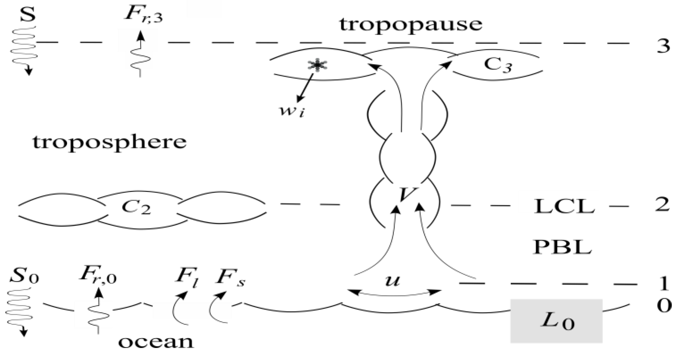
Figure 1. The model configuration of a coupled ocean/atmosphere, the latter consisting of a turbulent PBL topped by the LCL, where low clouds reside, and a free troposphere capped by tropopause where high clouds lie. The designated levels 0/1/2/3 are surface/anemometer-height/LCL/tropopause.
Climate 13 00116 g001
Figure 2. The thermal template (thin solid lines) and deduced climate properties (thick lines) plotted against the surface temperature (and its blackbody radiance) for the standard case of unit forcing. All variables are nondimensionalized (Appendix A). Thin dashed curves are LW fluxes from radiative transfer calculations. The light/dark shades indicate SW/LW cloud forcings, and the maximum turbulent wind (solid rectangle) specifies the surface temperature in accordance with MEP.
Climate 13 00116 g002
Figure 3. Vapor pressure versus temperature in the updraft (dashed), its ambient air (solid), and the saturated air (dotted). Subscripts 0/1/2 are for surface/anemometer-height/LCL. Td is the dew point, which defines the LCL.
Climate 13 00116 g003
Figure 4. Heat balances at the surface, the LCL and the tropopause for a given surface temperature. The LW flux at the LCL equals the surface one because of the shallow LCL (magnified tenfold). The low cloud reduces the surface LW flux and depletes the sensible heat flux. Open/solid arrows indicate responses to changing SW/LW forcings discussed in Section 3.1.
Climate 13 00116 g004
Figure 5. MEP-induced surface temperature plotted against the solar forcing spanning ±50% of the present solar constant. Boxed letters: H for Holocene, C for Cambrian/Cretaceous, A for Archean, A+ for Archean of high pCO2, and P for Precambrian with tropical supercontinents. Shaded is the model-derived tropical/polar temperature spread, whose intersections with the glacial marking temperature (GMT) (solid rec-tangles) specify thresholds for tropical/polar glaciations..
Climate 13 00116 g005
Figure 6. An illustration of the FYSP based on the TOA energy balance and fixed cloud albedo. The latter is tuned to match the present temperature (288 K, solid rectangle), which then yields a frozen surface (259 K, open rectangle) when the solar forcing S is reduced by 20%. Dashed and dash-dotted curves are OLRs lowered by the greenhouse effects of pCO2 or high-cloud cover (C3) to produce a surface temperature of 273 K (solid oval) and 288 K (open oval), respectively.
Climate 13 00116 g006
Figure 7. Same as Figure 2 but showing the change from Holocene to Archean climates (H → A, thick solid to dashed lines) when the solar constant decreases by 20%. The weaker forcing lowers the absorbed SW flux (S0), expands the high cloud (C3), and pushes the peak of the turbulent wind (u) to a lower temperature.
Climate 13 00116 g007
Figure 8. Same as Figure 7 but for the contrast of A → A+. Despite the forcing change being a small fraction of H → A, the temperature change is comparable in magnitude.
Climate 13 00116 g008
Figure 9. Same as Figure 8, but for the contrast of H → C. The high pCO2 has raised the surface temperature by 15 K from 288 to 303 K, attaining the observed warmth of the Cambrian/Cretaceous.
Climate 13 00116 g009
Disclaimer/Publisher’s Note: The statements, opinions and data contained in all publications are solely those of the individual author(s) and contributor(s) and not of MDPI and/or the editor(s). MDPI and/or the editor(s) disclaim responsibility for any injury to people or property resulting from any ideas, methods, instructions or products referred to in the content.