Article

The New IGRICE Model as a Tool for Studying the Mechanisms of Glacier Retreat

by
Pavel A. Toropov
1,2,
Anna A. Shestakova
3,4,5,*,
Anton Y. Muraviev
1,
Evgeny D. Drozdov
1,2 and
Aleksei A. Poliukhov
2,4,5
1
Institute of Geography of the Russian Academy of Sciences, Moscow 119017, Russia
2
Geography Faculty, Lomonosov Moscow State University, Moscow 119991, Russia
3
Obukhov Institute of Atmospheric Physics of the Russian Academy of Sciences, Moscow 119017, Russia
4
Research Computing Center, Lomonosov Moscow State University, Moscow 119234, Russia
5
Moscow Center for Fundamental and Applied Mathematics, Moscow 119991, Russia
*
Author to whom correspondence should be addressed.
Climate 2025, 13(12), 248; https://doi.org/10.3390/cli13120248
Submission received: 9 November 2025 / Revised: 8 December 2025 / Accepted: 9 December 2025 / Published: 11 December 2025

Abstract

Global glacier models (GGMs) are effective tools for assessing changes in water resources in mountainous regions and studying glacier degradation. Moreover, with the rapid development and increasing complexity of Earth System Models (ESMs), the incorporation of mountain glaciation parametrizations into ESMs is only a matter of time. GGMs, being computationally efficient and physically well-founded, provide a solid basis for such parametrizations. In this study, we present a new global glacier model, IGRICE. Its dynamic core is based on the Oerlemans minimal model, and surface mass balance (SMB) is explicitly simulated, accounting for orographic precipitation, radiation redistribution on the glacier surface, turbulent heat fluxes, and snow cover evolution on ice. The model is tested on glaciers situated in climatically and topographically contrasting regions—the Caucasus and Svalbard—using observational data for validation. The model is forced with ERA5 reanalysis data and employs morphometric glacial and topographic parameters. The simulated components of the surface energy and mass balance, as well as glacier dynamics over the period of 1984–2021, are presented. The model results demonstrate good agreement with observations, with correlation coefficients for accumulation, ablation, and total SMB ranging from 0.6 to 0.9. The primary driver of glacier retreat in the Caucasus is identified as an increase in net shortwave radiation balance caused by reduced cloudiness and albedo. In contrast, rapid glacier degradation in Svalbard is linked to an increased fraction of liquid precipitation and an extended snow-free period, leading to a sharp decrease in albedo.

1. Introduction

Mountain glacier meltwater contributes only a small fraction—less than 1% in average [1]—to river runoff compared to precipitation, evaporation, and snowmelt on lowlands. Nevertheless, accounting for mountain glaciers is essential for accurately modeling the hydrological regime in high mountain regions [2,3]. For example, glacier-fed river runoff in Central Asia can account for up to 50% of the annual river discharge [4]. Considering that the globally averaged decline in mountain glacier areas is about 1% per year [2], mountain glaciation of the Earth may disappear by the beginning of the 22nd century. This poses serious challenges for freshwater availability, potentially leading to economic crises and humanitarian disasters in some countries, thus making water resource management critically important [5]. The rapid reduction in mountain glacier volumes in the 20th–21st centuries is driving an increase in natural hazards in high mountain regions and will also lead to a noticeable rise in global mean sea level, as already shown in [6]. In addition, changes in glacier areas in major mountain systems affect regional climate primarily via alterations in surface albedo, available melt energy, and mesoscale atmospheric circulation patterns. For instance, Shaw et al. [7] demonstrated that large glaciers and, in general, mountain-glacier regions currently serve to moderate warming by cooling near-surface air and by generating katabatic winds. However, with further reduction in glacier area, warming rates in the mountains are expected to accelerate substantially. Consequently, developing physically based representations of mountain glacier systems remains highly relevant.
At present, glacier modeling addresses two primary tasks: (1) incorporating glacier meltwater contributions into mountain river runoff [3,4], and (2) projecting changes in mountain glacier volume and area under ongoing global climate change, especially in the 21st century [2,6]. In addition, glacier models also provide insights into the physical mechanisms behind observed and modeled changes in surface mass balance (SMB). One of the main manifestations of modern climate change in mountains is the upward shift in the equilibrium line altitude. This can be related to changes in the atmospheric heat content [8]. However, the real mechanisms of this shift differ substantially across regions, ranging from trends in the radiative flux component to changes in turbulent fluxes and precipitation characteristics (both amount and phase).
There is growing demand to integrate mountain glaciers into Earth System Models (ESMs). In most current ESMs, mountain glaciers are treated either as permanent snow cover, or, less frequently, as a land ice surface type (e.g., [9]) without accounting for glacier evolution. Only a few regional models, such as REMO, implement SMB calculations for the fraction of a grid cell occupied by glaciers and permit dynamic changes in glacier area [10].
The magnitude of the climate response to the mountain cryosphere remains incompletely quantified. In a number of studies, e.g., [7,11], the possibility of a noticeable influence of the mountain cryosphere on regional climate has been demonstrated in the example of the sensitivity of the Indian monsoon to variations in the snow–ice area in the Tibetan–Himalayan region. In the 21st century, one of the main vectors of Earth science development is the increasing complexity of ESMs, which now include a detailed description of the land surface layer, soil, snow cover, vegetation, lakes, wetlands, and urbanized regions. Incorporating mountain glaciers naturally represents the next step in this progression.
This study presents a new model, IGRICE (Institute of Geography glacieR model of Intermediate ComplExity). This model was intended as a prototype for mountain glacier parameterization in Earth System Models, which is also suitable for simulating individual glaciers and for studying the mechanisms of their degradation. Conceptually, the proposed IGRICE model is designed to be one of the so-called global glacier models (GGMs) in the sense that it should be applicable to any region and to any glacier. Such models consist of mass balance and a dynamical block. The latter simulates the response of glacier geometry (length, area, and volume) to changes in SMB. The complexity of the dynamical block in GGMs can vary from simple statistical parameterizations [12] or calibrated mass-balance boundary models [13] to one-dimensional shallow-ice approximations [14,15]. Currently, there are several dozen GGMs worldwide, among which the most developed are OGGM, GloGEM, GloGEMflow, PyGEM, JULES, and HYOGA2 (see reviews [15,16]).
Another glacier modeling approach employs full models based on the Navier–Stokes equations for viscoplastic flow driven by gravity. Numerous comparisons with field data have shown that such complex models can successfully simulate a single glacier [17,18] or ice-sheet dynamics. However, this approach requires scrupulous tuning of parameters for a particular glacier and entails high computational costs, limiting its applicability at regional or global scales.
SMB is a key component in glacier modeling, and there are currently two approaches to describing ablation and accumulation in models: (1) statistical and (2) energy balance. The statistical approach relies on empirical relationships between mass-balance components and climatic and topographic parameters (e.g., [19]). This method includes the widely used T-index approach, relating ablation to air temperature. Obvious advantages of the method are its computational cheapness and the ability to estimate ablation for any mountain glacier region without detailed meteorological measurements. Therefore, it is actively developed today [20,21,22] and is used both for climate interpretation of modern glacier degradation and for simulating the state of mountain glaciers by the end of the 21st century worldwide [2]. The main drawback of the method is the use of numerous empirical regression parameters, which hide the underlying physics of the interactions between heat-balance components. In contrast, the energy-balance approach is more physically grounded, calculating SMB components based on simplified energy conservation equations at the glacier surface. Accumulation is primarily derived from precipitation, while ablation results from the residual energy available for melting. Nowadays, so-called distributed energy-balance models with varying degrees of complexity have become widely used (e.g., [23,24,25,26]).
Accurately modeling accumulation on mountain glaciers requires considering orographic precipitation effects. Usually, accumulation is estimated from the coarse reanalysis fields after bias correction with measurements of snow depth, using both satellite data and ground-based measurements [6]. Accounting for snow redistribution on the glacier surface—by wind and avalanches—remains challenging and often requires high-resolution modeling [27] and remote sensing data [28]. Despite substantial progress in solving this task, there is not yet a conceptual model that relates precipitation, snow drift, and avalanche feeding with morphometric topography parameters [29].
Thus, in creating a new GGM for subsequent use as a parameterization of mountain glaciation in ESMs, we chose approaches that combine, on the one hand, simplicity and computational efficiency, and on the other hand, physically consistent representation of key SMB processes. The new model is based on an energy-balance approach and a parameterization of orographic precipitation (a “slope-model” type), while the dynamical block is represented by the minimal Oerlemans model. To ensure universality and transferability, the number of calibration parameters is minimized, and the model is designed to operate with climate forcing with coarse spatial resolution.
The IGRICE model is now under development, and in this paper, we present the first results of testing the current model version developed for individual glaciers. Thus, this paper represents a case study of a simulation of four individual glaciers in two different regions (Svalbard and the Caucasus), while development and testing of the model in a fully global framework is planned for the near future.
Section 2 provides a detailed description of the proposed model. Section 3 describes the experimental setup for four glaciers, where the model is tested. Section 4 presents the model results and their discussion, focusing on the physical mechanisms of changes in glacier mass balance, and Section 5 discusses the prospects for the model’s development.

2. IGRICE Model Description

2.1. General Scheme of the Model

The most optimal approach to modeling mountain glaciation is the “intermediate-complexity” method, which underpins the majority of GGMs. This approach effectively combines computational efficiency with a solid physical basis, which, in perspective, allows it to be used both for studying individual glaciers and within ESMs. One example of such an approach is the “minimal” Oerlemans model [8], which is used as a dynamical core of the IGRICE model. The main equation for glacier evolution is formulated as follows:
d V d t = 3 α m 2 1 + ν t a n ( θ N , g l ) L 1 / 2 W + α 2 L 1 α e α L L 1 e α L d L d t + α m 1 + ν t a n ( θ N , g l ) L 3 / 2 α 2 L 2 + e α L + α 2 L 2 e α L +   α 1 L 1 e α L d L d t = B s
Here, V and L are the glacier volume and length, respectively; W is the glacier front width; α m and ν are constants that define the simplified glacier dynamics (for most glaciers, α m = 3 , ν = 10 ); θ N ,   g l is the mean glacier surface slope (°); α is the scaling parameter of the modeled glacier, determining its geometry; and B s is the glacier SMB, determined by meteorological parameters. In the IGRICE model, B s is estimated based on the calculation of the main components of the heat and water budgets. The minimal model is integrated with a time step of 1 year using the simplest Euler scheme. The other blocks of the model can be integrated with a time step from 1 to 6 h (to resolve the diurnal cycle of solar radiation).
The schematic representation of the IGRICE model is depicted in Figure 1. This box model is implemented in FORTRAN and features a modular structure, enabling the straightforward integration of new components. In addition to the glacier dynamics module (Equation (1)), the model includes several other blocks, and the most important among them are the following: the module for calculating orographic precipitation, the snow evolution model, the input data preprocessing block, the radiation module (which recalculates radiative fluxes on the sloped glacier surface), the turbulent fluxes module, and the ice melt module. Most processes that influence accumulation and ablation on the glacier are calculated to a greater or lesser extent explicitly (such as snow dynamics, orographic precipitation, solving the energy-balance equation, etc.); however, some processes are currently parameterized using simple relationships (see Section 2.6). The output parameters of the IGRICE model are as follows: the components of the energy and mass balance, the evolution of the glacier length, area, and volume.
The IGRICE model requires input meteorological data at isobaric levels, surface radiation fluxes, and a set of geographic data on the topography and glacier morphometry. The isobaric data include the following: air temperature, specific and/or relative humidity, three components of wind speed, the specific moisture content of hydrometeors (snow and rain), and optionally, a cloudiness factor. Radiation data encompass incoming longwave radiation and incoming direct and diffuse shortwave radiation (separately). The geographic data include the following: general convexity of topography (convex/concave), the main azimuth of the glacier, the distribution of altitudinal zones and their fractional areas, glacier slope in each zone, maximum elevation and average slope of the topography in a given neighborhood/grid cell, and the fraction of debris in the lowest zone in the ablation season. A set of elevation angles for all azimuths (in 10-degree increments) for each glacier’s altitudinal zone is also required.
A prototype of the IGRICE model without the snow-cover module and with a simplified orographic precipitation parametrization was already tested on the Djankuat Glacier [30]. A good match was shown for a number of parameters including mass-balance components.
The following subsections provide a more detailed description of the main components of the model.

2.2. Orographic Precipitation

We use an orographic precipitation parameterization of the slope-model type, of which there are quite many [31]. Such an approach combines physical justification with simplicity. The proposed parameterization is based on calculation of the condensation rate on the windward mountain slope from temperature, humidity, and wind speed data at standard isobaric levels [32]:
ρ w   t = E R w T 2 L e R w T 1   w ( γ γ a )
Here, ρ w = E / R w T is the density of saturated water vapor; E is the saturation pressure; T is air temperature; L e is the latent heat of vaporization; R w = 461.5 J/(kg·K) is the specific gas constant for water vapor; γ a is the moist adiabatic lapse rate; γ = T z ; and w is the vertical velocity of an air parcel (m/s), determined as the sum of the large-scale (synoptic) and orographic components. In this work, the large-scale component of w is taken from reanalysis data under the assumption that the terrain within the grid cell is aggregated and does not generate mesoscale disturbances in the vertical velocity. That is, the vertical velocity in the reanalysis data is primarily determined by synoptic processes rather than by orography (at least at the scale of a single cell). The orographic component is obtained from a simplified continuity equation written for an incompressible fluid. On the glacier surface it is prescribed as follows:
w o 0 = c d v p t a n θ N , c e l l
where v p is the projection of the horizontal wind vector onto the glacier azimuth, θ N , c e l l is the slope angle of the surface (the average terrain slope in grid cell), and c d is an empirical coefficient. The physical interpretation of the latter is that it provides a simple account for the effect of three-dimensionality of orographic obstacles on the atmospheric flow. In the case of an idealized, infinitely long two-dimensional ridge of uniform height with no gaps, c d = 1 , meaning all the air mass flows directly over the ridge. The real topography is three-dimensional, and only a portion of the airflow passes over the obstacle, while the rest flows around it (especially for a bell-shaped mountain with an aspect ratio close to unity like Mt. Elbrus or Mt. Kilimanjaro) or through passes and canyons. We set c d to 0.5 for glaciers situated in concave topographical forms (which are usually located on mountain ridges with moderate three-dimensionality) and to 0.25 for glaciers on convex terrain (usually substantially three-dimensional terrain).
It is assumed that the height dependence of the orographic component of vertical velocity is primarily determined by atmospheric stratification conditions:
w o ( z ) = w o 0 e α o N 2 ( z ) δ h
where δ h is the height above the glacier surface,   N 2 is the Brunt–Väisälä frequency, and α o is an empirical constant representing an additional acceleration related to air resistance. Equation (4) suggests that vertical velocity attenuates with height as the air parcel moves away from the slope that generated this disturbance. In reality, orography can also generate internal gravity waves, which may cause vertical velocity to increase with height. However, accounting for gravity wave effects is a complex task and is beyond the scope of this study.
Using the empirical link between temperature and the fraction of condensed moisture that precipitates, and integrating the obtained moisture content through the entire column with depth Z , the total orographic precipitation on the windward side of the slope over the time interval t is obtained:
q w = t t + t 0 Z δ p δ C ρ w t d z d t
Here, δ C and δ p are empirical weighting functions [33]: δ C is the fraction of moisture that condensates depending on relative humidity, and δ p is the fraction of condensed moisture that precipitates.
Orographic precipitation is added to the large-scale grid-cell precipitation. The latter are computed as the product of air density, terminal velocity, and the specific content of hydrometeors (snow and rain) in the lower layer adjacent to the glacier (separately for each altitudinal zone). The terminal velocity is calculated separately for snow and rain using the parameterization by Lin et al. [34].
Previous studies [35,36] have demonstrated that the proposed precipitation module adequately reproduces the spatial and temporal variability of precipitation on the mountain slopes of the Caucasus and Kamchatka Peninsula. The accuracy of precipitation modeling was evaluated by comparing model results with observations and reconstructions of annual snow accumulation on the Western Plateau of Mt. Elbrus [32].

2.3. Snow-Cover Model

Currently, the Noah-MP land surface model [37], modified for glaciers by Michael Barlage, is used to calculate evolution of snow cover on glaciers. The IGRICE model incorporates the version of Noah-MP used in the WRF 4.1.2 model [38]. It includes three snow layers and four underlying ice layers.
The Noah-MP model includes several algorithms for separating precipitation into liquid and solid; BATS and CLASS snow albedo parameterizations; two methods for specifying the lower boundary condition; two snow/ice temperature time schemes; and an option for accounting for phase transitions in ice.
To ensure proper interaction with other modules in the IGRICE model, some modifications were made to the Noah-MP model. Specifically, ice albedo was reduced to values more typical for this environment: from 0.8 in the visible spectrum and 0.55 in the infrared to 0.4 and 0.25, respectively. Two additional parametrizations of snow albedo [39,40] have been added. A variation of the BATS snow albedo parameterization has been added, with constants selected in [41]. We also added an option to calculate turbulent exchange coefficients with stability functions from [42]. The ice layer thicknesses have been significantly increased compared to the standard version (totaling up to 130 m instead of the standard 2 m) to prevent complete melting of the ice during long simulations.

2.4. Energy Fluxes

The energy-balance module in IGRICE consists of two main blocks: the radiation block and the block for calculating turbulent fluxes (Figure 1).
A correct calculation of the ablation layer of mountain glaciers is impossible without taking into account the redistribution of incoming solar radiation as a function of slope orientation, its steepness, and topographical shading. We used a well-known Kondratyev relationship in the formulation [43] to calculate the direct solar radiation on the glacier surface:
S s ( z ) = S · m a s k s h a d o w [ cos Θ N s i n Θ S + s i n Θ N c o s Θ S cos ϕ S ϕ N ]
where S s is the direct radiation on the tilted surface; S is the direct radiation on the surface perpendicular to the sun’s rays; Θ S is the sun height; Θ N is the slope angle; ϕ S is the Sun’s azimuth; and ϕ N is the slope’s azimuth. A binary mask m a s k s h a d o w is used to indicate the presence or absence of shadow (0 when shadow and 1 when no shadow).
The diffuse radiation was calculated with the account for sky view factor s v f :
D S = D · s v f
where D is the diffuse solar radiation from input data. s v f was calculated from the elevation angles. It is zero when the horizon is completely closed and unity when it is completely open.
If the height of the glacier altitudinal zone and the height for which radiation input data are available do not coincide (in reanalysis, the height of the surface is typically significantly lower than the glacier height), we perform a correction for incoming shortwave and longwave radiation:
S c ( z ) = S s ( z ) γ s z
L W ( z ) = L W s + ( L W c l e a r ( z ) L W c l e a r ,   s )
Here, S c ( z ) and L W ( z ) are the corrected incoming shortwave and longwave radiation fluxes, respectively; L W s and L W c l e a r ,   s are the incoming longwave radiation and longwave radiation under clear-sky conditions, respectively, at the input data height (in our case, the height of the surface in reanalysis). z is the height difference between the glacier height and the input data height; γ s is an empirical gradient of incoming shortwave radiation, which for mountain systems of mid-latitudes, based on measurements and modeling, is taken as −2.5 W m−2 per 100 m [31]. The dependence of longwave radiation on height is not known, so in our model we only corrected the clear-sky part of longwave radiation flux. The height dependence of L W c l e a r is proposed in [44] and validated on glaciers of Mt. Elbrus [45]:
L W c l e a r z = A T c ( z ) + B Q ( z ) + C
where T c is air temperature in °C, Q is moisture content (cm) integrated in the air column above a given level z , and A , B , and C are constants equal to 2.8, 0.25, and 199.9, respectively.
We also included an option to account for the thermal radiation from rocks and moraines adjacent to the glacier [46]:
L W r o c k = ε σ ( T r o c k 4 T s 4 ) s i n Θ N , r o c k 2
Here, the rock emissivity ε = 0.99 , σ is the Stefan Boltzman constant, T r o c k is the rock surface temperature (for now set constant for each glacier), T s is the glacier surface temperature, and Θ N , r o c k is the slope angle of rocks (for now, set as the mean value for each glacier). This parameterization works only in the presence of direct solar radiation (taking topographical shadowing into account) and positive air temperature.
For calculating turbulent heat fluxes at the glacier surface, the standard bulk formulas are used:
H = ρ c p C t C u U θ a θ s   ;   L E = ρ L e C q C u U q a q s    
Here, H and L E are turbulent fluxes of sensible and latent heat; θ a and θ s are the potential air temperatures in the surface layer and at the surface; q a and q s are the specific humidities in the surface layer and at the surface; U is the wind speed magnitude in the surface layer; C u , C t , and C q are the turbulent exchange coefficients for momentum, heat, and moisture, respectively; c p is the specific heat capacity of air at constant pressure; and ρ is air density.
Currently, two options are available for calculating the exchange coefficients: the standard Businger–Dyer functions [47] and the functions by Grachev et al. [42], tuned for conditions of stable stratification above snow and ice. The dynamic roughness parameter is set as a constant (2 mm for snow and 1 mm for ice [25]), and the thermal roughness is computed according to [48]. The algorithm for calculating turbulent exchange coefficients is from the surface-layer SFX model, developed jointly by Russian Computing Center of the Lomonosov Moscow State University and Institute of Numerical Mathematics of the Russian Academy of Sciences [49].

2.5. Ice Ablation Module

To calculate ice ablation when snow is gone, we did not use the Noah-MP model. Firstly, the ice in this model is treated more like soil than like glacier [50], and secondly, solving the full heat conduction equation in ice to determine surface ablation during the melting season is excessive for our purposes. Instead, we used a simple algorithm with the following assumptions, which are appropriate for glaciers during the period of active melting [51]. (1) The heat flux into the glacier due to molecular diffusion, G , is small and is approximated as a constant value of 5 W m−2, consistent with in situ measurements and the results of modeling based on measurements [21,25]. (2) The surface temperature during the ablation season cannot exceed 0 °C. (3) Heat flux from liquid precipitation is neglected due to its small contribution compared to other energy-balance components [23,46]. Based on these assumptions, the complete heat-balance equation for the ice surface simplifies to the following equation:
L i ρ i h t = S W 1 A + L W + L W r o c k L W + H + L E + G
Here, h is the thickness of the ice layer (ice ablation layer); ρ i is the ice density (917 kg m−3); L i is the specific heat of melting/freezing (333.5 kJ kg−1); A is the broadband ice albedo; and L W is the outgoing longwave radiation flux from the surface.

2.6. Some Other Parametrizations

Some processes in the model are currently represented in less detail than those described above. However, these processes can be significant, and more detailed parameterizations are planned for future versions of the model. This primarily applies to snow redistribution caused by snowdrift events, variations in ice albedo depending on ice contamination and snowmelt time, and the evolution of the debris cover.
Numerous studies have shown that precipitation is the main factor feeding mountain glaciers, accounting for about 80% of their mass gain globally [51,52]. Avalanches contribute on average about 5%, and snowdrifts about 15%, although for some individual glaciers these factors can account for more than 50% of the total accumulation. In the current version of the IGRICE model, a characteristic percentage of avalanche feeding is prescribed for each glacier. Snowdrift transport and accumulation in concave landforms are currently represented by a so-called “concentration coefficient” (a factor multiplying precipitation amount), which is defined as the approximate ratio of the glacier basin’s area to the glacier area [53] and is also adjusted depending on glacier type. Thus, for glaciers on conical peaks, typical of Mt. Elbrus, this value is close to 1 on average. It equals 0.7–0.8 in the upper morphological zones, where the snow is blown away by the wind without any hindrance, and 1.2–1.3 near the tongue, where the wind is weaker and moraine ridges trap snow. For mountain–valley glaciers (which account for approximately 80% of the Earth’s mountain glaciers), the concentration coefficient ranges from 1.5 to 2.5 depending on topography and wind conditions. Since IGRICE is developed as a future parametrization module for ESMs, it is envisaged to develop a parameterization of snowdrift transport that explicitly accounts for wind speed, wind direction, and terrain geometry (as is demonstrated, for example, in [28]).
Ice albedo A is currently parameterized using simple linear relationships between reflectivity and the proportion of debris on ice and the number of days since snow disappearance a g e i :
A = A i 1 f r d + A d f r d ;   A i = A i , y o u n g 1 a g e i / a g e r e f ;   A = m a x ( A , A m i n )
Here, A i is the albedo of pure ice, A i , y o u n g is the albedo of pure ice immediately after snow disappearance (set to 0.5), A d is the debris albedo (set to 0.15), f r d is the fraction of debris on ice, a g e r e f is the typical duration of a snow-free period on a glacier (set to 45 days), and A m i n = 0.07 is the minimum possible ice albedo. The debris fraction is set for the lowest altitudinal zone based on observation data on each glacier and decreases linearly above, so that it is zero in the uppermost zone.
On many glaciers, the presence of a thick debris cover on the ice surface can play a significant role in mass balance, slowing or completely stopping ice melting in areas where moraine material accumulates [54,55]. The IGRICE model currently uses a simple algorithm from [56] to account for this effect. In the presence of a debris cover, the ablation value is multiplied by a coefficient f h d e b r i s that varies from 0 to 1.65 and depends on the cover thickness H Z , t :
f h d e b r i s =   K d e b r i s +   H c r i t K d e b r i s +   H Z , t , i f   H Z , t > H e f f
f h d e b r i s = K d e b r i s + H c r i t K d e b r i s + H e f f H Z , t H e f f + H e f f H Z , t H e f f , i f   H Z , t H e f f
where H e f f = 0.02 m (the layer depth of thin debris that increases melting), H c r i t = 0.04 m (the layer depth of thick debris that increases melting), and K d e b r i s = 0.1 .

3. Selected Glaciers and Model Set-Up

3.1. Selected Glaciers

The proposed model was tested on glaciers listed in the World Glacier Monitoring Service, which are considered representative of their regions and relatively well studied. We selected two mountain-glacier regions with contrasting climatic conditions: the Northern Caucasus situated at the boundary between temperate continental and maritime subtropical climates, and the Svalbard archipelago, characterized by a maritime subarctic climate.
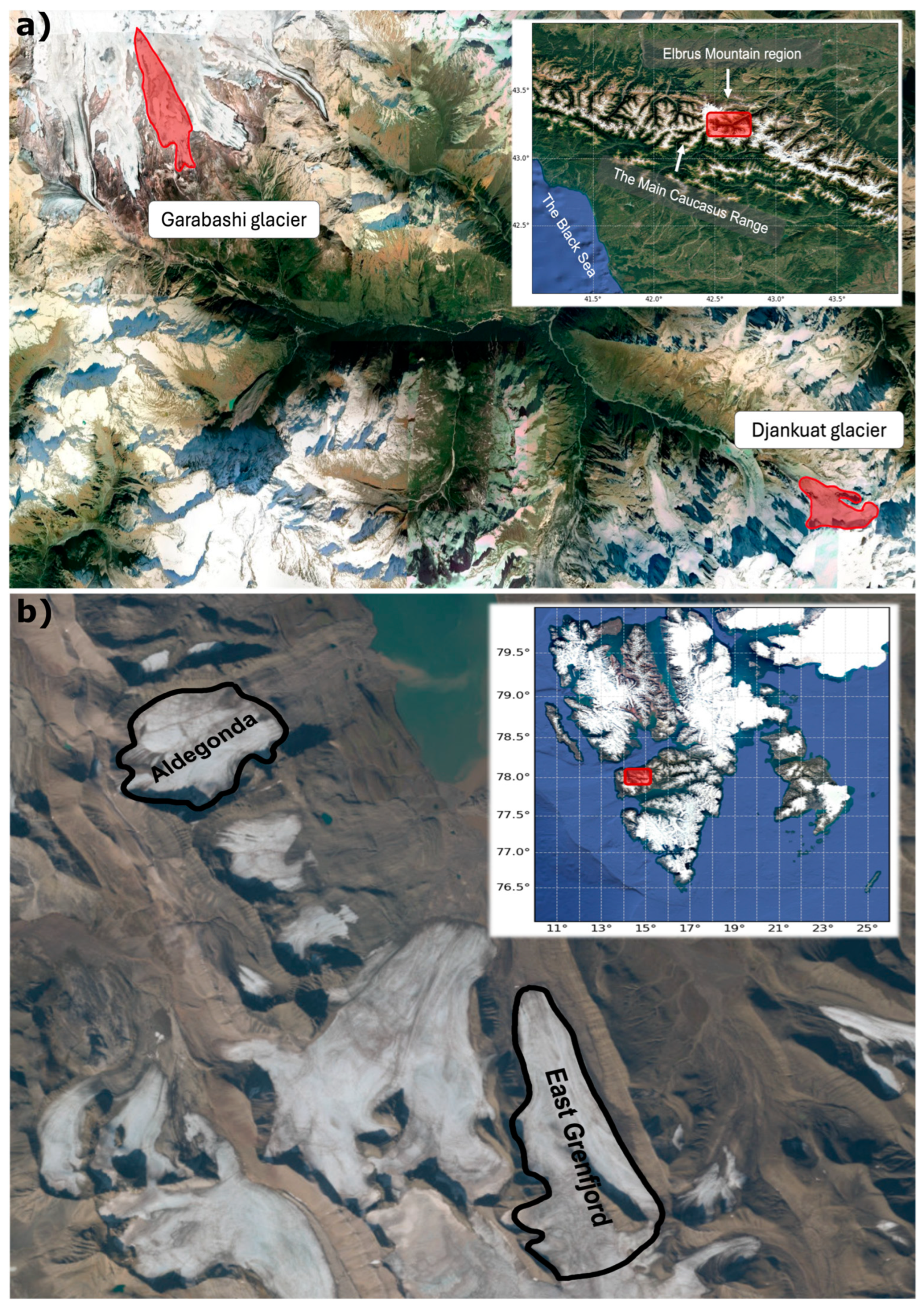
Within each region, we chose two glaciers with different exposition and that were sufficiently well studied: the Djankuat and Garabashi glaciers in the Caucasus, and the Aldegonda (Aldegondabreen) and East Grønfjord (Austre Grønfjorden) glaciers Svalbard (Figure 2).
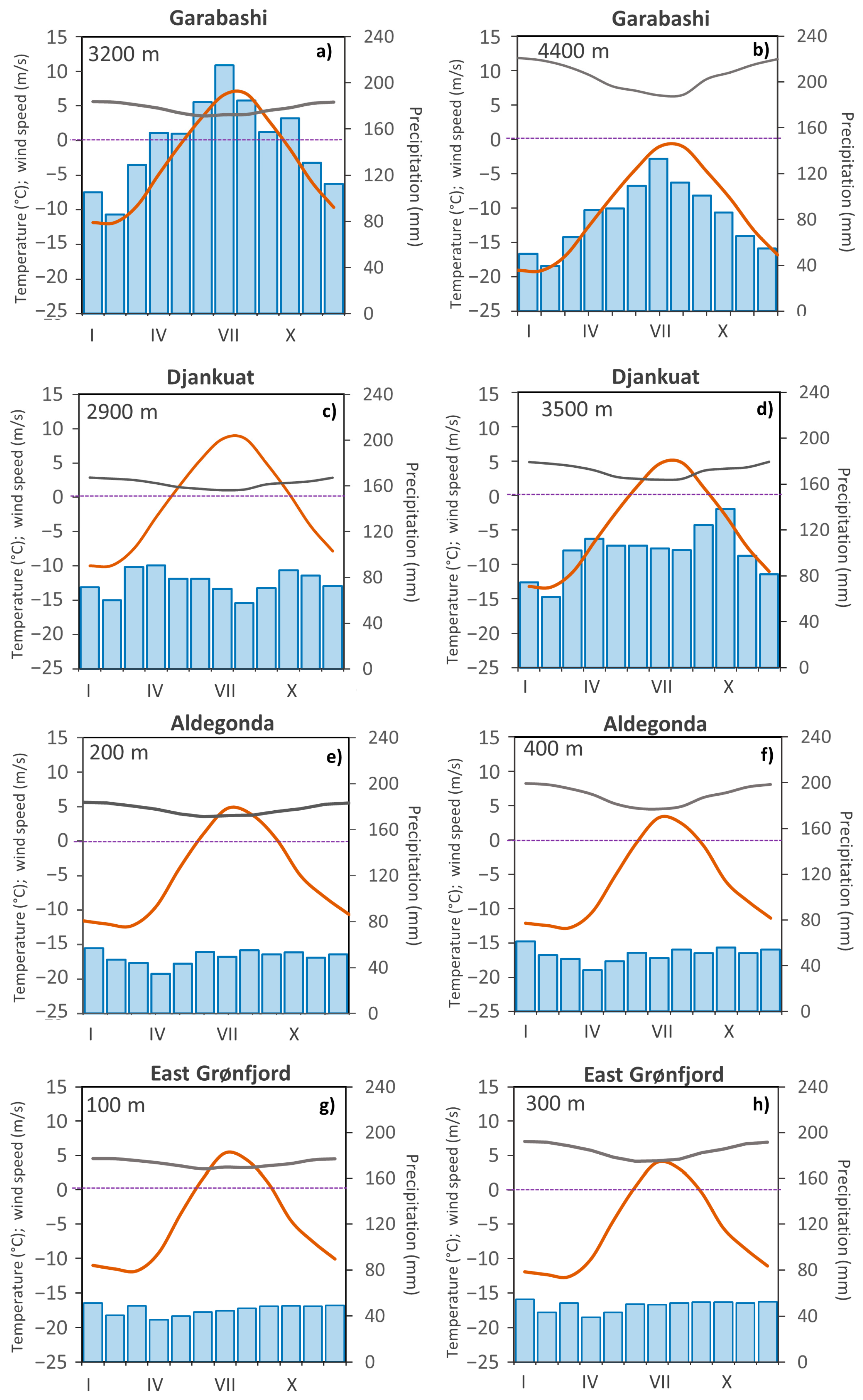
The Djankuat Glacier is the most extensively studied glacier in Russia. Mass-balance measurements have been carried out here since 1967 [57], and since 2008, a comprehensive set of meteorological and hydrological measurements have been conducted simultaneously [58]. It is a relatively small valley glacier located on the northwestern slope of the Main Caucasus Range (Figure 2a). Its parameters are typical of the Central Caucasus: in 1968, its area was 3.2 km2 and its length 3450 m. Over the last 40 years, the glacier has degraded considerably: its length and area have decreased by about 15%. According to ERA5 reanalysis data, the air temperature in the lowest zone of the Djankuat glacier is positive from May to October, while in the upper zone, positive air temperatures prevail from mid-June to mid-September (Figure 3). The modeled annual precipitation cycle is quite smooth, reflecting the relatively uniform moistening of the Main Caucasus Range throughout the year, which is typical for a maritime subtropical climate.
The Garabashi Glacier is also located in the Caucasus and has undergone a similar retreat in recent years. It lies on the southeastern slope of Mt. Elbrus, at elevations between 3200 and 4400 m above sea level (m a.s.l.), within microclimatic conditions contrasting with the Djankuat Glacier. According to ERA5 reanalysis, the mean annual wind speed reaches 10 m/s in the upper zone of this glacier, and the average monthly air temperature in July remains below 0 °C; maximum monthly precipitation sums reach 120 mm even at 4400 m a.s.l. (Figure 3). Overall, modeled precipitation on the Garabashi Glacier is nearly twice that on the Djankuat Glacier. The Garabashi Glacier belongs to the ice cap type and is characterized by a rather convex surface and a smaller snow concentration coefficient (due to wind erosion), as well as smaller values of avalanche feeding and debris fraction. Another characteristic feature of the Garabashi Glacier is the maximum elevation difference between its lowest and highest points, exceeding 1200 m. the Garabashi Glacier is relatively large for the Caucasus even under current dramatic glacier retreat conditions: its current length is 5500 m, and its area is about 4 km2. The glacier has been continuously monitored since 1986 [59].
Svalbard glaciers exhibit markedly different climatic conditions, typical of the mountainous archipelago in the Western Arctic. According to observations at the nearest Barentsburg weather station [60] and modeling results, there is a winter maximum in precipitation. However, the orographic amplification smooths the seasonal cycle for both glaciers (Figure 3c,d). Due to the small elevation range between the glacier terminus and the highest point, the air temperature changes only slightly with height and remains persistently positive from mid-May to mid-September according to ERA5 reanalysis (Figure 3).
The considered Svalbard glaciers differ from Caucasus ones not only by different climatic conditions but also in morphometric parameters. They are much more gently sloped (the surface slope angle is about half that of the Caucasus glaciers), the elevation difference is 3–4 times smaller (200–300 m), and the thickness and, consequently, the volume are substantially larger. At the same time, the rates of retreat in length and area for these glaciers are significantly higher than in the Caucasus: between 1990 and 2020, the fronts of Aldegonda and East Grønfjord retreated by 1000–1200 m, and their area decreased by 1.5–2 times. If these degradation rates persist, these glaciers could potentially disappear by 2060. Aldegonda is a cirque glacier with a northeast exposition; East Grønfjord is a valley glacier with north exposition. Glaciological monitoring at these glaciers is maintained by the Arctic and Antarctic Institute and by the Institute of Geography of the Russian Academy of Sciences [25,36].
Mass-balance modeling for Djankuat and East Grønfjord glaciers has been conducted previously. Moreover, a minimal Oerlemans model has been implemented for the Djankuat Glacier, albeit with prescribed measured mass-balance values [61]. Later, a numerical flow-line model similar to the one we use was employed to model the glacier dynamics, in which SMB was also partly specified from observations (from nearby weather stations, brought to the glacier level using empirical coefficients) and partly modeled in a simplified form [62]. The model successfully simulates glacier SMB after careful calibration. Model estimates showed that even under the most severe climate-warming scenario, the glacier would persist by the end of the 21st century, largely due to the accumulated debris cover preventing melting [62]. Mass balance on East Grønfjord was modeled using the distributed energy-balance model A-Melt [26], which includes a snow module; the model was forced with observations from nearby weather stations and satellite data, and the precipitation gradient was chosen as a result of model calibration.
T-index models were also used for reconstructing the mass balance of Aldegonda and East Grønfjord glaciers for individual years [26,60].

3.2. Description of Model Setup and Input Data

Numerical experiments with the IGRICE model, aimed at modeling the main mass-balance components and the geometric shape of the selected glaciers, were organized as follows:
  • Integration period: 1983–2021, time step of 3 h. The first year was not analyzed (model spin-up period). Annual mass balance was calculated at the end of the glaciological (mass balance) year, which for the Caucasus glaciers was taken as October 1, and for the Svalbard glaciers as September 1.
  • Input data: ERA5 reanalysis data (spatial resolution 0.25°) with a 3-h time step for the grid cell containing the glacier. The quality of ERA5 and its predecessor ERA-Interim for temperature and wind speed has been frequently evaluated for mountain regions, including the Caucasus, based on comparisons with meteorological measurements on glaciers (e.g., [30,63]). Satisfactory data quality for temperature and wind speed has been shown. In the Arctic, ERA5 also agrees reasonably well with observations at weather stations, though wind speed and relative humidity are reproduced worse than temperature and shortwave radiation [64].
  • Sources of general morphometric glacier characteristics: Catalog of Russian Glaciers [65], Randolph Glacier Inventory [66], as well as results from in situ measurements discussed above [25,26,57,59,60].
  • Topography data within the reanalysis grid cell used for the studied glaciers were obtained from processing the ASTER Global Digital Elevation Model (GDEM 3) [67] with a spatial resolution of 30 m (in a rectangular coordinate system). The same DEM was used to compute elevation angles for each of the altitudinal zones.
The main model parameters for the considered glaciers are given in Table 1, while the details of setting these and some other parameters are shown in Table S1 in Supplementary Materials. Most parameters were specified from stationary geodata (Table S1), while only the glacier dynamics parameters for the minimal Oerlemans model, along with some physical parameterization options and the snow concentration coefficient, were used to tune the model for each glacier, as discussed in more detail in the next Subsection. Section 5 discusses possible ways to parameterize these calibration parameters.

3.3. Selecting Some Model Parameters

The experiments conducted with the model showed that the modeling results are most sensitive to parameters that control snow melt, primarily the snow albedo parameterization, as was also found by [68]. As demonstrated by Abolafia-Rosenzweig et al. [41], the constants governing the albedo change with snow age in the BATS scheme can vary over a very wide range. Abolafia-Rosenzweig et al. [41] found an optimal set of parameters for this scheme by comparing with observations in the Rocky Mountains. We also found that this set of parameters from [41] yields adequate results for our glaciers; the calculated albedo is close to typical observed values. However, using BATS scheme even with this set of parameters results in too weak snow melt for Djankuat Glacier, where the accumulation is the biggest among all considered glaciers. We were obliged to multiply the snow-aging coefficients by 3 to obtain adequate results for this glacier.
Other snow albedo schemes, ref. [39,40,69], were tested as well. However, none of them proved universal, i.e., suitable for all glaciers. The CLASS scheme clearly yields a significantly overestimated albedo. It is possible that the problem lies not so much in the snow albedo parameterization but in the evolution of the physical characteristics of snow (primarily density and the fraction of liquid water in snow). Using different snow-aging albedo parameters for different glaciers is a limitation of this work, but it stems from the absence of the best parameterization of this process. In the future, a more detailed analysis and tuning of the snow model are planned, including testing different snow models.
In the snow model, we used parametrization [70] to separate precipitation into rain and snow (to which the model has no significant sensitivity), the condition of zero heat flux at the bottom of ice, a semi-implicit time scheme for temperature in ice and snow. Phase transitions in ice are switched on.
The snow concentration coefficient was specified based on both physical considerations and calibration against the observed mass balance in each zone. For instance, the low concentration coefficient values on the Garabashi Glacier are due to its strong convexity and location on Mt. Elbrus. The upper part of this glacier is exposed to strong winds, which blow away the snow. The Djankuat Glacier, by contrast, is located in a strongly concave relief, which, combined with high wind speeds in the upper part, leads to high snow concentration coefficient values. Precipitation blown from the southern macro-slope of the Caucasus may also play a significant role.
All experiments were performed using the stability functions [42] for turbulent exchange coefficients calculation, and the height of the surface layer (i.e., the height at which turbulent exchange coefficients and turbulent fluxes were computed) was set to 10 m. This last parameter has a large effect on the results; the choice of 10 m was driven mostly by the best agreement between modeled turbulent fluxes and observations, though this may be a coincidental alignment due to the influence of several factors and requires further testing. On the other hand, 10 m is a reasonable value for the surface layer above glaciers, especially for the ablation season when it is characterized by persistent stable stratification and katabatic winds that thin the constant-fluxes layer.

4. Results and Discussion

4.1. Mass Balance and Glacier Dynamics

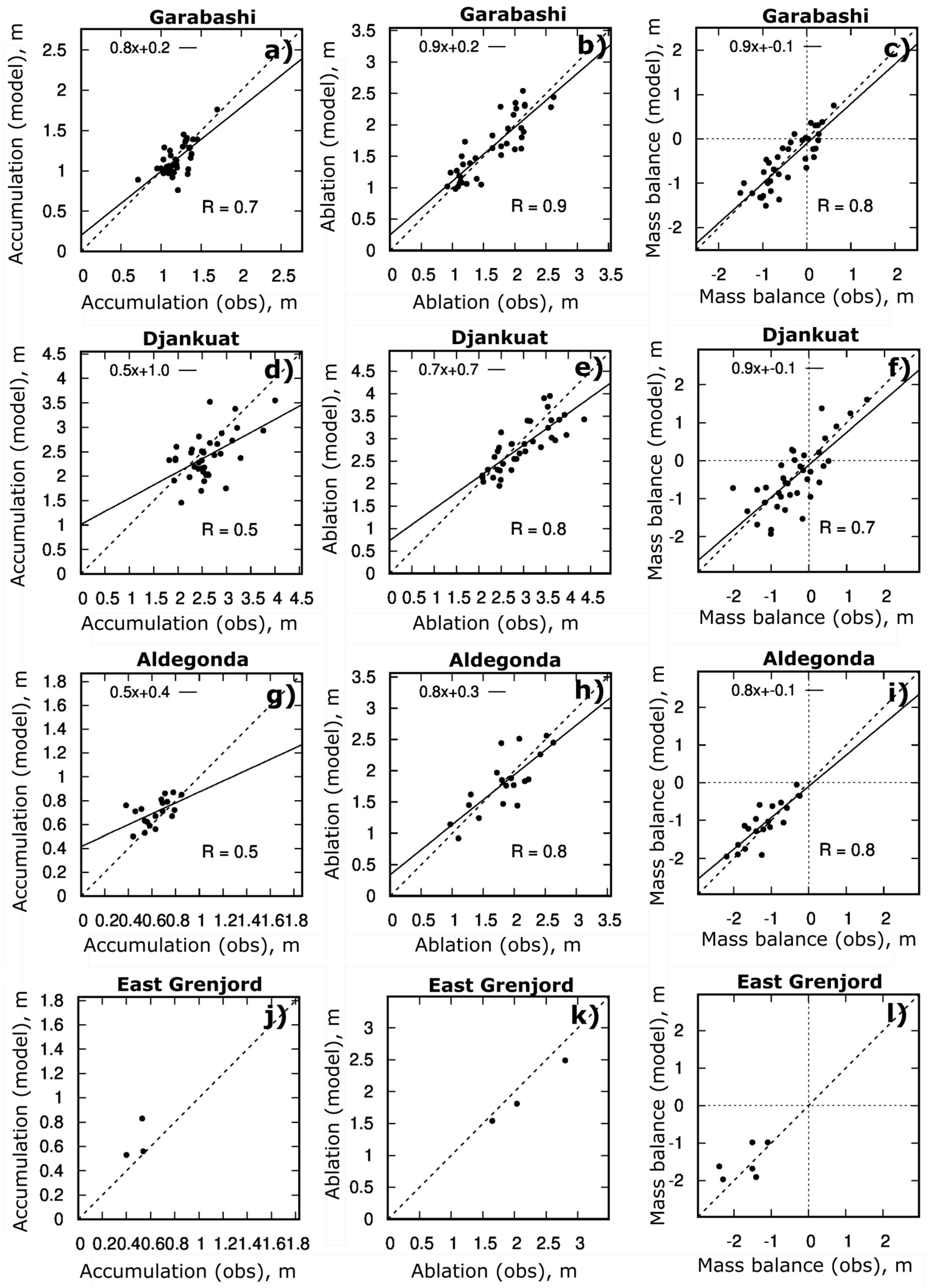
Results of glacier mass-balance modeling compared with observations are presented in Figure 4, Figure 5 and Figure 6. When comparing the modeled and observed mass-balance curves (Figure 4), it is important to note that the observed curves for three glaciers were obtained by averaging over a significantly shorter time period than the modeling period. Specifically, accurate observational data on the change in SMB with height are available for only 4 years (2018–2021) for the Garabashi Glacier, 5 years (2014, 2016–2019) for the East Grønfjord Glacier, and 8 years (2014–2021) for the Aldegonda Glacier. As can be seen, the observational data cover the most recent years when the balance was most negative. Therefore, the observed curves are close to the maximum (in absolute value) of the modeled mass-balance curves (Figure 4). Only for the Djankuat Glacier was the average mass-balance curve constructed from observations spanning a longer period, from 1968 to 2021. This explains why the modeled and observed curves are in good agreement for this glacier (Figure 4d–f), indicating that the model accurately reproduces the height dependence of SMB.
The modern climate changes have led to the disappearance of the accumulation zone on many glaciers. For the Garabashi Glacier, the mass balance in the upper zones averaged over 38 years is close to zero (Figure 4a). In the lower part of the glacier, within elevations of 3200–3800 m a.s.l., ablation is very large, averaging about 3.5 m w.e. per year (Figure 4b). Among all modeled glaciers, only the Djankuat Glacier still retains an accumulation zone (Figure 4c). However, observations [57] and modeling show the disappearance of snow cover during the melt season almost at all parts of the glacier in recent years. The accumulation zone on considered Svalbard glaciers has completely disappeared in the last 15 years. Now, all the snow accumulated during the winter (as well as the superimposed ice formed by refreezing) completely melts away over the summer [26]. The 10-year average of annual SMB values is approximately −1.5 m w.e., with extreme values reaching −2 m w.e. in some years [26].
The model reasonably reproduces the accumulation and ablation dynamics for the modeled glaciers (Figure 5), with a correlation coefficient of about 0.7–0.8 (Figure 6). Accumulation over the period of 1984–2021 changed little, while ablation increased significantly. In particular, ablation on considered Svalbard glaciers increased by nearly 1.5 times in 2001–2021 compared to 1984–1999. An increase in accumulation during the 2016–2021 period is noted from observations on the Djankuat Glacier. However, this increase is not statistically significant and could not compensate for the very high ablation during that period. Notably, in 2020, the observed ablation reached its maximum (4.4 m w.e.) over the entire observation period since 1967 [57]. The Svalbard glaciers exhibit negative simulated mass balance throughout the modeling period, losing their mass about 1.5 times faster than glaciers in the Central Caucasus.
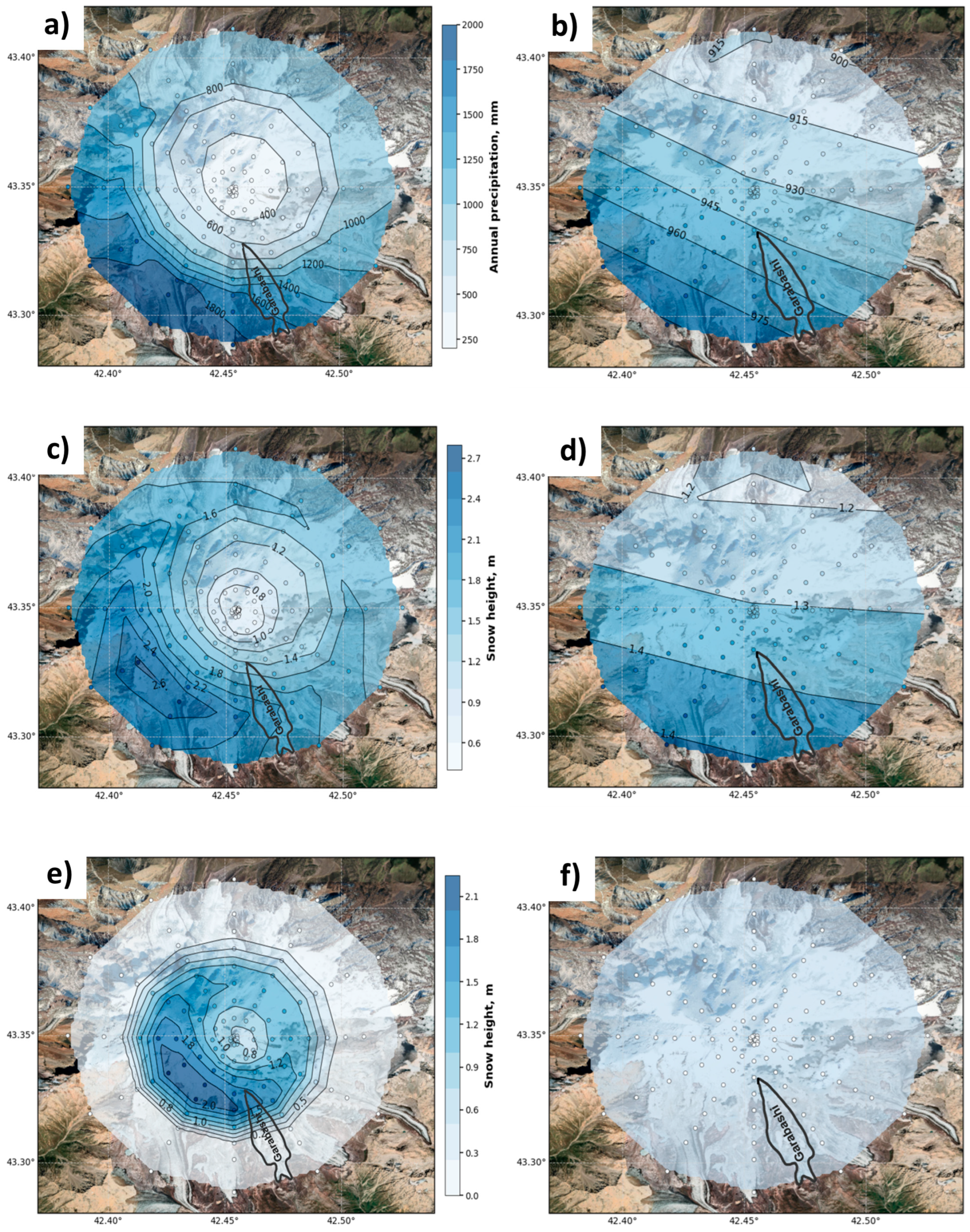
The ablation is reproduced particularly well, with a correlation coefficient of 0.8–0.9 (Figure 6). This can be explained by the fact that the main contribution to ablation comes from the radiative balance, which depends primarily on the geometry of the slopes and topographical shading, both of which can be set quite accurately in the model. Compared with the previous, more simplified version of the model used to simulate the Djankuat Glacier [30], the quality of ablation simulation has increased significantly (the correlation coefficient has increased from 0.6 to 0.8; the mean error has decreased by more than half). This improvement is due to many factors, including the addition of vertical zoning of the glacier, debris cover, longwave flux from rocks, correction of radiation with altitude, modifications in the calculation of turbulent exchange coefficients, and other factors. Accumulation on mountain glaciers is reproduced satisfactorily, but the model accuracy of this component is somewhat worse (correlation 0.5–0.7) than for ablation. The quality of representation of the accumulation on the Djankuat Glacier in the current version of the model and in the prototype [30] is almost the same, since the parameterization of orographic precipitation has changed relatively little. The accumulation field is best reproduced for the Garabashi Glacier (Figure 6a) since this glacier belongs to ice cap glaciers, for which the snow concentration factor is close to unity and the accumulation field is almost entirely determined by the precipitation field. Despite the lack of sufficient precipitation measurements in high mountain regions, one can say that precipitation is well represented by the model. Figure 7a,b illustrates an example of the simulated precipitation and snow depth on Mt. Elbrus, where the Garabashi Glacier is located. It is important to note that a realistic spatial pattern of precipitation distribution and snow depth is obtained almost without calibrating the model to measurements. The only empirical parameter is c d , which depends on the three-dimensionality of the terrain. For comparison, Figure 7c,d shows precipitation and snow depth from ERA5-Land reanalysis with 9 km spatial resolution [71]. Reanalysis is not able to reproduce the right precipitation gradient and underestimates precipitation amount on the southern macro-slope of Mt. Elbrus by about a factor of two. Overall, in the Central Caucasus, the modeled gradient for annual precipitation is about 0.5 mm/m in the height range 2500–3200 m a.s.l., and −0.7 mm/m above 3500 m a.s.l. The simulated maximum annual precipitation is located at 3200–3500 m a.s.l. and ranges from 1200 to 2000 mm (depending on slope exposure). This is in good agreement with the maximum snow accumulation in the Caucasus [72]. The maximum precipitation at 3000–3500 m a.s.l., amounting to 1500 mm, and a precipitation gradient of 0.5 mm/m are typical for mid-latitude mountain systems, particularly for the Alps [31], with similar climatic conditions. However, for glaciers with significant snow redistribution due to snowdrift (especially for Djankuat), it is clear that a more sophisticated accounting of the concentration coefficient is needed for accumulation modeling.
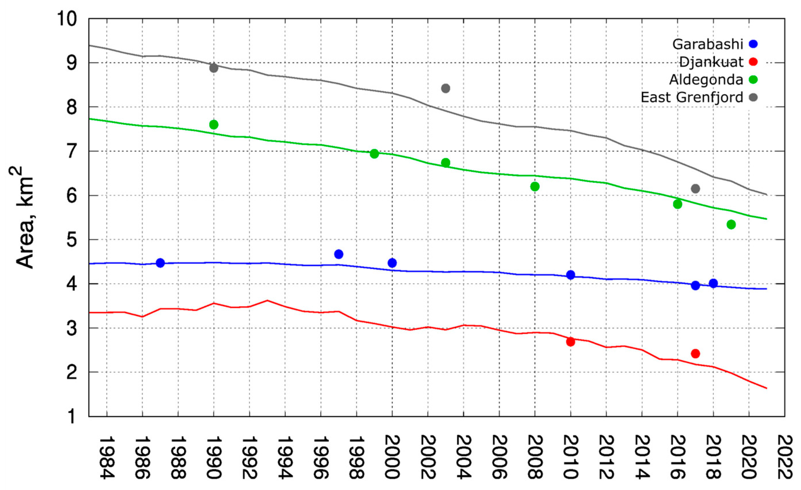
Glacier area is a key parameter in modeling mountain glaciation in the ESMs. The IGRICE model generally adequately reproduces the rapid area loss of glaciers in the Caucasus and in Svalbard (Figure 8). In most cases, the error is 3–5%, and only for the Garabashi Glacier it reached 10% in 1997. Apparently, the response of glacier area to SMB anomalies is essentially linear for the considered glaciers. Therefore, with a relatively accurate representation of mass-balance components, it is possible to obtain accurate glacier area dynamics. It should be noted that the minimal Oerlemans model does not take into account the influence of three-dimensional and nonlinear effects on glacier dynamics, which may be important for some glaciers, especially large ones. However, since most mountain glaciers on the Earth are similar in size to those considered in our study, it is believed that this model will perform satisfactorily on a global scale.

4.2. Mechanisms of Glacier Degradation

To understand the observed and modeled trends in the SMB of glaciers in the Caucasus and in Svalbard, we examine the heat-balance components, their trends, and correlation with ablation.
The lack of accumulation trends for all considered glaciers is due to the lack of trends in annual precipitation (Table 2). Changes in ablation, however, are driven by different factors for different glaciers. In general, variability in annual ablation is more closely related to variability in ice melt (correlation coefficient 0.85–0.98) than in snow melt.
According to the IGRICE model results, the main factor of ablation on all considered glaciers during the summer months is the radiation balance, specifically its shortwave part (Figure 9), which is consistent with observational data [25,73]. The share of radiation balance in the heat balance reaches 85–90% in the lower zones of the Caucasus glaciers.
The direct solar radiation in the Caucasus region significantly increases through the modeling period (more than 1.5 Wm−2 per decade), while glacier surface albedo significantly decreases (Table 3). As a result, the net shortwave radiation balance increases by approximately 2 W m−2 per decade, or by 7–8 W m−2 over the entire modeling period. Assuming an average length of a melt season of 120 days in this region, this increase in radiation balance is equivalent to an increase in melting of 240–270 mm w.e.
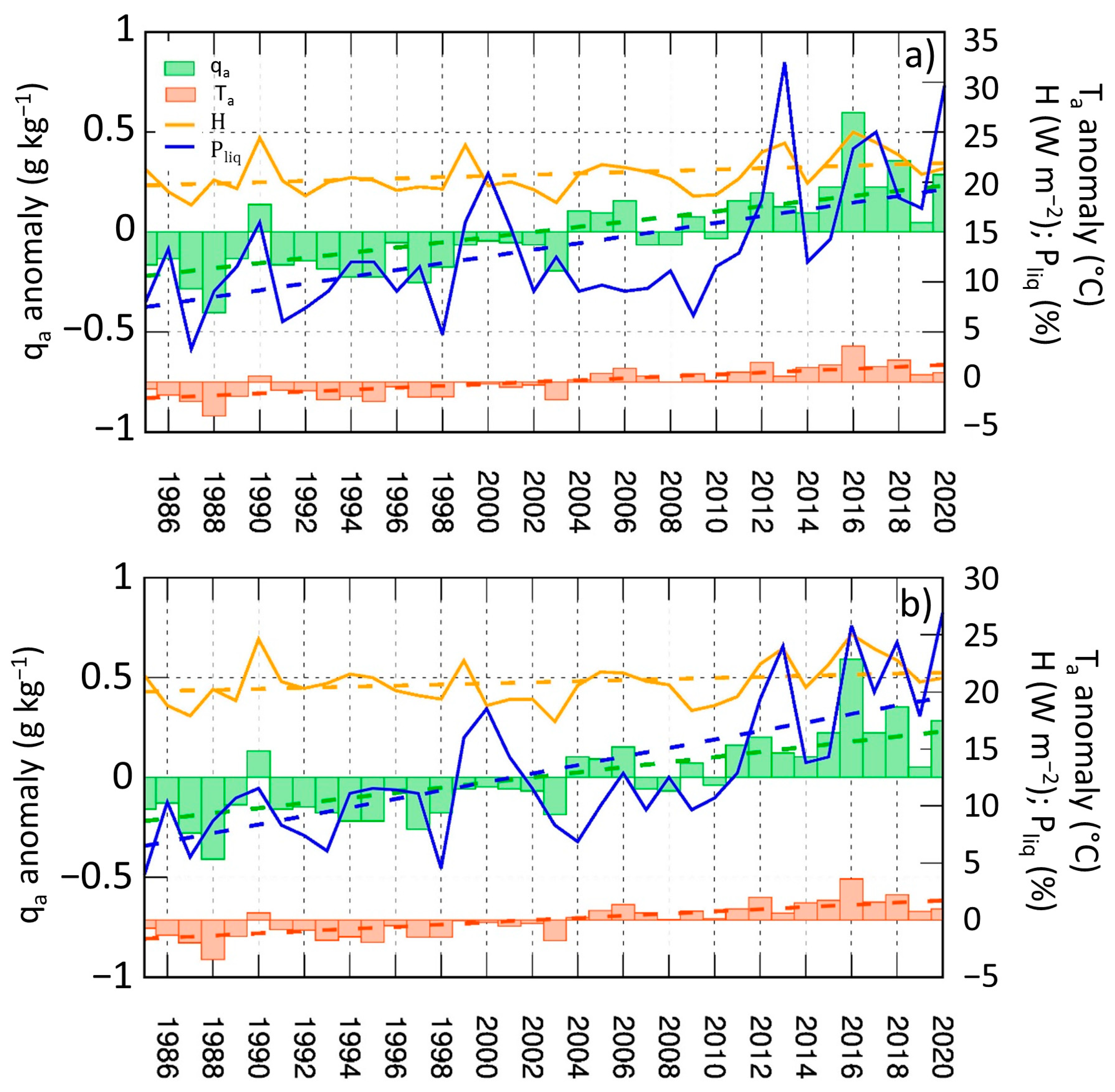
These changes in radiation fluxes are accompanied by a significant increase in atmospheric pressure (Table 2) and a decrease in cloudiness (Figure 10), which correspond to an increase in the frequency of anticyclonic circulations. This mechanism was discussed in [74] and is often associated with the so-called “tropical expansion”, the process of widening the descending branch of the Haddley cell and its northward shift against the background of ongoing climate change [75]. This process is quite clearly manifested near the Mediterranean Sea, where the Azores anticyclone dominates in the summer season. Another reason for the increase in incoming shortwave radiation may be a decrease in aerosol optical depth, which has been observed in recent decades in various regions [76,77]. This process manifests itself in two ways: on the one hand, a decrease in aerosols leads to an increase in the transmission of shortwave radiation, while on the other hand, it leads to a decrease in cloud water content, which also contributes to an increase in transmission.
For the Caucasus glaciers, we also found a statistically significant correlation between ablation and air temperature (0.6–0.7); the latter increases at a rate of 0.4 °C/10 years (Table 2). However, the mechanism by which temperature changes influence ablation is not entirely clear, as an increase in turbulent fluxes is very weak (Table 3), and the relationship between ablation and turbulent fluxes is statistically insignificant (Table 4). The contribution of turbulent fluxes to the heat balance in the Caucasus increases with altitude (Figure 9) and in winter becomes comparable to the radiation balance in the upper zones of glaciers. The role of heat loss due to evaporation and sublimation increases especially significantly with altitude: average monthly values on the Garabashi Glacier in the summer months are −50 to −55 W m−2. This is due to the combination of frequent strong winds with a large moisture deficit [45].
The role of net shortwave radiation balance in Svalbard is less pronounced than in the Caucasus (Figure 9). The slight increase in shortwave radiation balance there (Table 3) is not due to changes in incoming radiation, which remains relatively constant or even slightly decreases (due to diffuse radiation), but rather to a sharp decrease in surface albedo, at a the rate of −2% per decade (Table 3). Over 38 years, this resulted in an almost 8% reduction in surface albedo, equivalent to an additional melting of 105 mm w.e. of ice. The correlation between glacier mass balance and ablation and shortwave radiation balance is much weaker in Svalbard than in the Caucasus (Table 4).
The rate of increase in air temperature in Svalbard is more than twice that in the Caucasus (Table 2). This aligns with the well-known fact of higher warming rates in the Arctic compared to mid- and low-latitude regions, which is driven by the prevalence of temperature inversions and less intense vertical air mixing compared to other regions [78,79]. However, the correlation between ablation and temperature here is statistically insignificant (Table 4). At the same time, ablation is strongly correlated to increasing air humidity here. A natural response to the increasing heat and moisture content of the atmosphere is a significant increase in incoming longwave radiation on the Svalbard glaciers (Table 3), although this flux is almost completely negotiated by upward longwave radiation from the surface, resulting in a rather weak negative trend in net longwave radiation.
The role of turbulent fluxes in Svalbard is more significant than in the Caucasus (Figure 9). Østby et al. [68] found an increase in turbulent fluxes over Svalbard glaciers for the period of 1957–2014 and a significant correlation between ablation and turbulent fluxes in summer. However, our estimations show that the correlation between annual mean turbulent heat fluxes and ablation is insignificant (Table 4). The only exception is the Aldegonda Glacier, for which a significant correlation coefficient (0.6) was found between ablation and latent heat flux. However, the simulated latent heat flux does not exhibit a significant linear trend (Table 3) and therefore cannot explain the negative mass-balance trend.
The most pronounced factor influencing SMB changes in Svalbard is the increase in both the amount (Table 2) and the fraction (Figure 11) of liquid precipitation (Table 2), a trend also supported by observational data [80]. The fraction of liquid precipitation almost doubled over the modeling period: from 10% in the 1980s to 20%, or 120 mm/year, at the end of the period. This increase is associated with rising air temperature, as our model divides precipitation into phases depending on temperature [70], while the total precipitation on the Svalbard glaciers remains unchanged. It is important to note that throughout the entire modeling period, the Aldegonda and East Grønfjord glaciers remain below the equilibrium line; thus, their snow cover melts almost completely during the melt season. However, whereas in the 1980s the duration of the snow-free period was approximately 1 month (typically from mid-August to mid-September), during which the glacier lost no more than 300 mm w.e., now the snow-free period has extended to 2–2.5 months, with its onset shifting to early July. This earlier melting of snow is significantly facilitated by the increased frequency of rainfall events, which lead to additional heating and modifications in snow structure, as evidenced by the strong correlation between the fraction of liquid precipitation and ablation (Table 4). Surprisingly, Østby et al. [68] report that although ablation correlates with summer rainfall, glacier mass balance shows no relation to winter rains. This discrepancy with our results may be explained by the fact that their study examines the overall mass balance for the entire Svalbard archipelago. Glaciers in the northern part may not receive as much rain as those in the central and southern parts, and influence of rain on mass balance may be oppositional—increasing ablation due to additional heat while also contributing to further refreezing and accumulation. In the future, the frequency of atmospheric heat waves in Svalbard is expected to increase [81], which should contribute to further increases in liquid precipitation and accelerate glacier retreat.

5. Prospects for the IGRICE Model Development

Despite some successes of the IGRICE model, significant work to refine the model and prepare it for inclusion in an ESM as a parametrization of mountain glaciers is planned for the future. This future work includes the following: (i) refining the model’s physics, (ii) preparing the input geodata (primarily topographical and glacier morphometric parameters) for the model, and (iii) testing the model in all major mountain-glacial regions.
Some important processes that are currently specified in the model as parameters (Table S1) require physical or statistical parameterization to improve the model’s performance and to increase its versatility. Among them is the process of snow redistribution due to snowdrift transport. At present, this process is described in the model by a concentration coefficient, constant for each glacier (Table S1). In the future, we plan to include a physically based parameterization of snow concentration on the glacier surface depending on the glacier type, the shape of the glacier surface, and the bedrock profile, e.g., [27,28,29].
Other planned improvements to the model’s physics include parameterization of avalanche feeding and debris cover evolution. A possible solution for unifying the snow albedo scheme is the development of a new parameterization that would incorporate the geographical location of glaciers. The glacier dynamics parameters for the minimal Oerlemans model will be parameterized based on glacier morphometric data.
We also plan to take into account some other important processes. The katabatic glacier wind is an example of such a process. These winds are observed on most mountain glaciers during the ablation period and significantly affect wind speed and, consequently, turbulent fluxes [82,83]. Models and reanalyses with coarse resolution, which are the main input data sources for our model, underestimate wind speed over glaciers due to their inability to reproduce mountain–valley circulation and glacier winds in particular. Even a simple scaling of wind speed from the coarse grid improves the results of turbulent flux simulation over glaciers [84]. The surface layer height parameterization we plan to include should also be related to the katabatic wind effect.
There are a number of other subtle effects that can be important in glacier modeling but are not accounted for in global models. For example, daytime cloud formation due to mountain–valley circulation, which can significantly reduce the radiation balance, as well as orographic convection, which occurs on slopes exposed to the sun for most of the day (primarily southern slopes). All of this will improve the simulation of mass-balance components and their dynamics.
Another necessary step is to create a special database with main subgrid topography and glacier parameters for each azimuth aggregated for each grid cell of ERA5 reanalysis and, in the future, of the Russian climate model INMCM (Institute of Numerical Mathematics Climate Model) [85]. Further, a “hypothetical glacier” with typical parameters for each azimuth in a grid cell will be constructed on the basis of this database. The proposed glacier model would simulate the SMB and dynamics of this “hypothetical glacier” and return updated glacier parameters to the climate model each year.
Testing the improved version of the model in areas with different climatic and geographic conditions around the globe will help select the optimal set of parameterizations for physical processes and fine-tune the model’s operation.

6. Conclusions

This paper presents a new global glacier model, IGRICE. Our aim was to develop a model with a relatively small number of parameters that captures the most important features of the meteorological regime over a glacier. The model was tested on glaciers in contrasting climate conditions—the Caucasus and Svalbard—and produced satisfactory results. The correlation coefficients between measured and modeled annual mass balance are 0.70–0.80, with a mean bias of 6 cm for Caucasus glaciers and 11 cm for Svalbard glaciers. The model reproduces the vertical distribution of mass balance and its components with altitude.
Simulation results from the IGRICE model for the period of 1984–2021 were used to investigate the physical mechanisms of glacier degradation in detail. In the Caucasus, the main driver of increased ablation was a decrease in surface albedo accompanied by a substantial increase in direct solar radiation, likely related to an increased frequency of anticyclonic events in the region. In Svalbard, the principal mechanism is a longer snow-free period, largely due to a significant increase in the fraction of liquid precipitation.
A key advantage of the IGRICE model is its ability to study glacier degradation mechanisms. Many existing GGMs employ a T-index approach to estimate glacier ablation, with glacier accumulation calibrated using remote sensing and field measurements. These approaches are effective and widely used in modern glaciology [2,6,21]. However, they are sensitive to calibration coefficients derived from observational data, which poses challenges when considering past or future climate scenarios. Moreover, the T-index approach does not allow for identification of the underlying physical mechanisms governing glacier dynamics. Climate change manifests not only as a rise in temperature but also through changes in humidity, cloudiness, shortwave and longwave radiation fluxes, precipitation, and other factors that vary regionally, affecting glacier SMB in different ways.
The proposed model could become an effective tool for assessing glacier-fed river runoff and freshwater resources in mountain regions, as well as for identifying the physical mechanisms underlying glacier dynamics across various regions, both in past climatic epochs and under various global warming scenarios. In the future, we plan to incorporate the IGRICE model into the INMCM Earth System Model [85] to parameterize mountain glaciation.

Supplementary Materials

The following supporting information can be downloaded at: https://www.mdpi.com/article/10.3390/cli13120248/s1, Table S1: The main user-defined parameters of IGRICE model are categorized by type.

Author Contributions

Conceptualization, P.A.T.; methodology, P.A.T., A.A.S., A.Y.M., E.D.D., and A.A.P.; software, A.A.S.; validation, P.A.T. and A.A.S.; formal analysis, P.A.T. and A.A.S.; writing—original draft preparation, P.A.T. and A.A.S.; writing—review and editing, P.A.T. and A.A.S.; visualization, A.A.S. and E.D.D.; supervision, P.A.T.; project administration, P.A.T.; funding acquisition, P.A.T. All authors have read and agreed to the published version of the manuscript.

Funding

The development and validation of the IGRICE model was supported by the Russian Science Foundation, grant No. 23-17-00247. The development of the orographic precipitation parametrization and testing of the snow cover model for Mt. Elbrus was funded by the Russian Science Foundation, grant No. 24-17-00152.

Data Availability Statement

The ERA5 data are available at https://cds.climate.copernicus.eu/datasets/reanalysis-era5-pressure-levels?tab=overview (accessed on 8 December 2025). The IGRICE model is currently privately available at https://github.com/shestakova-aa-92/IGRICE, but will soon be made publicly available.

Acknowledgments

The authors thank A.M. Smirnov for providing mass-balance observations for the Garabashi Glacier.

Conflicts of Interest

The authors declare no conflicts of interest. The funders had no role in the design of the study; in the collection, analyses, or interpretation of data; in the writing of the manuscript; or in the decision to publish the results.

References

  1. Doganovsky, A.M. Land Hydrology (General Course); Russian State Hydrometeorological University: St. Petersburg, Russia, 2012; 524p. (In Russian) [Google Scholar]
  2. Huss, M.; Hock, R. Global-scale hydrological response to future glacier mass loss. Nat. Clim. Change 2018, 8, 135–140. [Google Scholar] [CrossRef]
  3. Rets, E.; Khomiakova, V.; Kornilova, E.; Ekaykin, A.; Kozachek, A.; Mikhalenko, V. How and when glacial runoff is important: Tracing dynamics of meltwater and rainfall contribution to river runoff from headwaters to lowland in the Caucasus mountains. Sci. Total Environ. 2024, 927, 172201. [Google Scholar] [CrossRef] [PubMed]
  4. Sorg, A.; Bolch, T.; Stoffel, M.; Solomina, O.; Beniston, M. Climate change impacts on glaciers and runoff in Tien Shan (Central Asia). Nat. Clim. Change 2012, 2, 725–731. [Google Scholar] [CrossRef]
  5. Zhupankhan, A.; Tussupova, K.; Berndtsson, R. Water in Kazakhstan, a key in Central Asian water management. Hydrol. Sci. J. 2018, 63, 752–762. [Google Scholar] [CrossRef]
  6. Huss, M.; Hock, R. A new model for global glacier change and sea-level rise. Front. Earth Sci. 2015, 3, 664–682. [Google Scholar] [CrossRef]
  7. Shaw, T.E.; Miles, E.S.; McCarthy, M.; Buri, P.; Guyennon, N.; Salerno, F.; Carturan, L.; Brock, B.; Pellicciotti, F. Mountain glaciers recouple to atmospheric warming over the twenty-first century. Nat. Clim. Change 2022, 15, 1212–1218. [Google Scholar] [CrossRef]
  8. Oerlemans, J. Minimal Glacier Models; Igitur: Utrecht, The Netherlands, 2008; 91p. [Google Scholar]
  9. Tolstykh, M.A.; Fadeev, R.Y.; Shashkin, V.V.; Goyman, G.S. Improving the Computational Efficiency of the Global SL-AV Numerical Weather Prediction Model. Supercomput. Front. Innov. 2021, 8, 11–23. [Google Scholar] [CrossRef]
  10. Kotlarski, S.; Jacob, D.; Podzun, R.; Frank, P. Representing glaciers in a regional climate model. Clim. Dyn. 2010, 34, 27–46. [Google Scholar] [CrossRef]
  11. Jin, L.; Ganopolski, A.; Chen, F.; Claussen, M.; Wang, H. Impacts of snow and glaciers over Tibetan Plateau on Holocene climate change: Sensitivity experiments with a coupled model of intermediate complexity. Geophys. Res. Lett. 2005, 32, 360–390. [Google Scholar] [CrossRef]
  12. Carlson, B.Z.; Georges, D.; Rabatel, A.; Randin, C.F.; Renaud, J.; Delestrade, A.; Zimmermann, N.E.; Choler, P.; Thuiller, W. Accounting for tree line shift, glacier retreat and primary succession in mountain plant distribution models. Divers. Distrib. 2014, 20, 1379–1391. [Google Scholar] [CrossRef]
  13. Raper, S.C.B.; Braithwaite, R.J. Glacier volume response time and its links to climate and topography based on a conceptual model of glacier hypsometry. Cryosphere 2009, 3, 183. [Google Scholar] [CrossRef]
  14. Hutter, K. The application of the shallow-ice approximation. Theor. Glaciol 1983, 1, 256–332. [Google Scholar]
  15. Zekollari, H.; Huss, M.; Farinotti, D.; Lhermitte, S. Ice-Dynamical Glacier Evolution Modeling—A Review. Rev. Geophys. 2022, 60, e2021RG000754. [Google Scholar] [CrossRef]
  16. Postnikova, T.N.; Rybak, O.O. Global glaciological models: A new stage in the development of methods for predicting glacier evolution. Part 1. General approach and model architecture. Ice Snow 2021, 62, 620–636. (In Russian) [Google Scholar] [CrossRef]
  17. Rybak, O.O.; Rybak, E.A.; Kutuzov, S.S.; Lavrentyev, I.I.; Morozova, P.A. Calibration of the mathematical model of the dynamics of the Marukh glacier, Western Caucasus. Ice Snow 2015, 55, 9–20. (In Russian) [Google Scholar] [CrossRef][Green Version]
  18. Reichert, B.K.; Bengtsson, L.; Oerlemans, J. Recent glacier retreat exceeds internal variability. J. Clim. 2002, 15, 3069–3081. [Google Scholar] [CrossRef]
  19. Steiner, D.; Walter, A.; Zumbuhl, H.J. The application of a non-linear back-propagation neural network to study the mass balance of Grosse Aletschgletscher, Switzerland. J. Glaciol. 2005, 51, 313–323. [Google Scholar] [CrossRef]
  20. Hock, R. Temperature index melt modelling in mountain areas. J. Hydrol. 2003, 282, 104–115. [Google Scholar] [CrossRef]
  21. Ohmura, A. Physical basis for the temperature-based melt-index method. J. Appl. Meteorol. 2001, 40, 753–761. [Google Scholar] [CrossRef]
  22. Wheler, B.A.; Flowers, G.E. Glacier subsurface heat-flux characterizations for energy-balance modeling in the Donjek Range, southwest Yukon, Canada. J. Glaciol. 2011, 57, 121–133. [Google Scholar] [CrossRef]
  23. MacDougall, A.H.; Flowers, G.E. Spatial and temporal transferability of a distributed energy-balance glacier melt-model. J. Clim. 2011, 24, 1480–1498. [Google Scholar] [CrossRef]
  24. Lozano Gacha, M.F.; Koch, M. Distributed Energy Balance Flux Modelling of Mass Balances in the Artesonraju Glacier and Discharge in the Basin of Artesoncocha, Cordillera Blanca, Peru. Climate 2021, 9, 143. [Google Scholar] [CrossRef]
  25. Prokhorova, U.; Terekhov, A.; Ivanov, B.; Demidov, V. Heat balance of a low-elevated Svalbard glacier during the ablation season: A case study of Aldegondabreen. Arct. Antarct. Alp. Res. 2023, 55, 2190057. [Google Scholar] [CrossRef]
  26. Elagina, N.; Kutuzov, S.; Rets, E.; Smirnov, A.; Chernov, R.; Lavrentiev, I.; Mavlyudov, B. Mass balance of Austre Grønfjordbreen, Svalbard, 2006–2020, estimated by glaciological, geodetic and modeling approaches. Geosciences 2021, 11, 78. [Google Scholar] [CrossRef]
  27. Bernhardt, M.; Liston, G.E.; Strasser, U.; Zängl, G.; Schulz, K. High resolution modelling of snow transport in complex terrain using downscaled MM5 wind fields. Cryosphere 2010, 4, 99–113. [Google Scholar] [CrossRef]
  28. Wayand, N.E.; Marsh, C.B.; Shea, J.M.; Pomeroy, J.W. Globally scalable alpine snow metrics. Remote Sens. Environ. 2018, 213, 61–72. [Google Scholar] [CrossRef]
  29. Freudiger, D.; Kohn, I.; Seibert, J.; Stahl, K.; Weiler, M. Snow redistribution for the hydrological modeling of alpine catchments. Wiley Interdiscip. Rev. Water 2017, 4, e1232. [Google Scholar] [CrossRef]
  30. Toropov, P.A.; Debol’skii, A.V.; Polyukhov, A.A.; Shestakova, A.A.; Popovnin, V.V.; Drozdov, E.D. Oerlemans minimal model as a possible instrument for describing mountain glaciation in earth system models. Water Resour. 2023, 50, 675–687. [Google Scholar] [CrossRef]
  31. Barry, R.G. Mountain Weather and Climate, 3rd ed.; Cambridge University Press: Cambridge, UK, 2008; 506p. [Google Scholar]
  32. Toropov, P.A.; Shestakova, A.A.; Yarinich, Y.I.; Kutuzov, S.S. Modeling Orographic Precipitation Using the Example of Elbrus. Izv. Atmos. Ocean. Phys. 2023, 59, S8–S22. [Google Scholar] [CrossRef]
  33. Sinclair, M.R. A Diagnostic Model for Estimating Orographic Precipitation. J. Appl. Meteorol. 1994, 33, 1163–1175. [Google Scholar] [CrossRef][Green Version]
  34. Lin, Y.L.; Farley, R.D.; Orville, H.D. Bulk parameterization of the snow field in a cloud model. J. Appl. Meteorol. Climatol. 1983, 22, 1065–1092. [Google Scholar] [CrossRef]
  35. Sushintsev, I.M.; Drozdov, E.D.; Toropov, P.A.; Mikhalenko, V.N.; Vorobiev, M.A.; Hayredinova, A.G. Modeling of snow cover on glaciers of the Caucasus and Kamchatka Peninsula. Ice Snow 2025, 65, 21–36. (In Russian) [Google Scholar]
  36. Elagina, N.; Rets, E.; Korneva, I.; Toropov, P.; Lavrentiev, I. Simulation of mass balance and glacial runoff of Mount Elbrus from 1984 to 2022. Hydrol. Sci. J. 2025, 70, 1929–1949. [Google Scholar] [CrossRef]
  37. Niu, G.Y.; Yang, Z.L.; Mitchell, K.E.; Chen, F.; Ek, M.B.; Barlage, M.; Kumar, A.; Manning, K.; Niyogi, D.; Rosero, E.; et al. The Community Noah Land Surface Model with Multiparameterization Options (Noah-MP): 1. Model Description and Evaluation with Local-Scale Measurements. J. Geophys. Res. Atmos. 2011, 116, D12109. [Google Scholar] [CrossRef]
  38. WRF v. 4.1.2 Source Code. Available online: https://github.com/wrf-model/WRF/releases/tag/v4.1.2 (accessed on 9 November 2025).
  39. Turkov, D.V.; Drozdov, E.D.; Lomakin, A.A. Snow albedo and its parameterization for the purposes of modeling natural systems and climate. Izv.—Atmos. Ocean. Phys. 2024, 60, 240–253. [Google Scholar] [CrossRef]
  40. Oerlemans, J.; Greuell, W. Sensitivity studies with a mass balance model including temperature profile calculations inside the glacier. Z. Für Gletscherkunde Glazialgeol. 1986, 22, 101–124. [Google Scholar]
  41. Abolafia-Rosenzweig, R.; He, C.; McKenzie Skiles, S.; Chen, F.; Gochis, D. Evaluation and optimization of snow albedo scheme in Noah-MP land surface model using in situ spectral observations in the Colorado Rockies. J. Adv. Model. Earth Syst. 2022, 14, e2022MS003141. [Google Scholar] [CrossRef]
  42. Grachev, A.A.; Andreas, E.L.; Fairall, C.W.; Guest, P.S.; Persson, P.O.G. SHEBA flux-profile relationships in the stable atmospheric boundary layer. Bound.-Layer Meteorol. 2007, 124, 315–333. [Google Scholar] [CrossRef]
  43. Muller, M.D.; Scherer, D. A grid-and subgrid-scale radiation parameterization of topographic effects for mesoscale weather forecast models. Mon. Weather Rev. 2005, 133, 1431–1442. [Google Scholar] [CrossRef]
  44. Nezval, E.I.; Chubarova, N.E.; Gröbner, J.; Ohmura, A. Influence of atmospheric parameters on long-wave downward radiation and features of its regime in Moscow. Izv. Atmos. Ocean. Phys. 2012, 48, 610–617. [Google Scholar] [CrossRef]
  45. Mikhalenko, V.N.; Kutuzov, S.S.; Lavrentyev, I.I.; Toropov, P.A.; Abramov, A.A.; Aleshina, M.A.; Gagarina, L.V.; Doroshina, G.Y.; Zhino, P.; Kozachek, A.V.; et al. Glaciers and Climate of Elbrus; Nestor-History Publishing House: St. Petersburg, Russia, 2020; 372p. (In Russian) [Google Scholar]
  46. Voloshina, A.P. Meteorology of Mountain Glaciers. Data Glaciol. Stud. 2002, 92, 3–138. (In Russian) [Google Scholar]
  47. Businger, J.A.; Wyngaard, J.C.; Izumi, Y.; Bradley, E.F. Flux-Profile Relationships in the Atmospheric Surface Layer. J. Atmos. Sci. 1971, 28, 181–189. [Google Scholar] [CrossRef]
  48. Kazakov, A.L.; Lykosov, V.N. Parametrization of Atmosphere–Land Surface Interactions in Numerical Modeling of Atmospheric Processes. Proc. West Sib. Reg. Res. Inst. 1982, 55, 3–20. (In Russian) [Google Scholar]
  49. Mortikov, E.V.; Debolskiy, A.V.; Glazunov, A.V.; Chechin, D.G.; Shestakova, A.A.; Suiazova, V.I.; Gladskikh, D.S. Planetary boundary layer scheme in the INMCM Earth system model. Russ. J. Numer. Anal. Math. Model. 2024, 39, 343–352. [Google Scholar] [CrossRef]
  50. Eidhammer, T.; Booth, A.; Decker, S.; Li, L.; Barlage, M.; Gochis, D.; Rasmussen, R.; Melvold, K.; Nesje, A.; Sobolowski, S. Mass balance and hydrological modeling of the Hardangerjøkulen ice cap in south-central Norway. Hydrol. Earth Syst. Sci. 2021, 25, 4275–4297. [Google Scholar] [CrossRef]
  51. Cuffey, K.M.; Paterson, W.S.B. The Physics of Glaciers, 4th ed.; Academic Press: Cambridge, MA, USA, 2010; 704p. [Google Scholar]
  52. Turchaninova, A.S.; Lazarev, A.V.; Marchenko, E.S.; Seliverstov, Y.G.; Sokratov, S.A.; Petrakov, D.A.; Barandun, M.; Kenzhebaev, R.; Saks, T. Methods of snow avalanche nourishment assessment (on the example of three Tian Shan glaciers). Ice Snow 2019, 59, 460–474. [Google Scholar] [CrossRef]
  53. Krenke, A.N.; Ananicheva, M.D.; Demchenko, P.F.; Kislov, A.V.; Nosenko, G.A.; Popovnin, V.V.; Khromova, T.E. Glaciers and glacial systems. In Methods for Assessing the Consequences of Climate Change for Physical and Biological Systems; Federal State Budgetary Institution “Research Center “PLANETA”: Moscow, Russia, 2012; 508p. [Google Scholar]
  54. Lambrecht, A.; Mayer, C.; Hagg, W.; Popovnin, V.; Rezepkin, A.; Lomidze, N.; Svanadze, D. A comparison of glacier melt on debris-covered glaciers in the northern and southern Caucasus. Cryosphere 2011, 5, 525–538. [Google Scholar] [CrossRef]
  55. Rounce, D.R.; Hock, R.; McNabb, R.W.; Millan, R.; Sommer, C.; Braun, M.H.; Malz, P.; Maussion, F.; Mouginot, J.; Seehaus, T.C.; et al. Distributed global debris thickness estimates reveal debris significantly impacts glacier mass balance. Geophys. Res. Lett. 2021, 48, 2020GL091311. [Google Scholar] [CrossRef] [PubMed]
  56. Compagno, L.; Huss, M.; Miles, E.S.; McCarthy, M.J.; Zekollari, H.; Pellicciotti, F.; Farinotti, D. Modelling supraglacial debris-cover evolution from the single glacier to the regional scale: An application to High Mountain Asia. Cryosphere 2021, 16, 1697–1718. [Google Scholar] [CrossRef]
  57. Popovnin, V.; Gubanov, A.; Lisak, V.; Toropov, P. Recent mass balance anomalies on the Djankuat glacier, Northern Caucasus. Atmosphere 2024, 15, 107. [Google Scholar] [CrossRef]
  58. Rets, E.P.; Popovnin, V.V.; Toropov, P.A.; Smirnov, A.M.; Tokarev, I.V.; Chizhova, J.N.; Budantseva, N.A.; Vasil’Chuk, Y.K.; Kireeva, M.B.; Ekaykin, A.A.; et al. Djankuat glacier station in the North Caucasus, Russia: A database of glaciological, hydrological, and meteorological observations and stable isotope sampling results during 2007–2017. Earth Syst. Sci. Data 2019, 11, 1463–1481. [Google Scholar] [CrossRef]
  59. Rototaeva, O.V.; Nosenko, G.A.; Kerimov, A.M.; Kutuzov, S.S.; Lavrentiev, I.I.; Kerimov, A.A.; Nikitin, S.A.; Tarasova, L.N. Changes in the mass balance of the Garabashi glacier (Mt. Elbrus) at the turn of the XX-XXI centuries. Ice Snow 2019, 59, 5–22, (In Russian with English Summary). [Google Scholar]
  60. Terekhov, A.; Prokhorova, U.; Verkulich, S.; Demidov, V.; Sidorova, O.; Anisimov, M.; Romashova, K. Two decades of mass-balance observations on Aldegondabreen, Spitsbergen: Interannual variability and sensitivity to climate change. Ann. Glaciol. 2023, 64, 225–235. [Google Scholar] [CrossRef]
  61. Kunakhovich, M.G.; Makarov, A.V.; Popovnin, V.V. Response of the Djankuat Glacier to Expected Climate Changes (According to the Oerlemans Model). Bulletin of Moscow University. Series 5,Geography 1996, 1, 31–37. (In Russian) [Google Scholar]
  62. Verhaegen, Y.; Huybrechts, P.; Rybak, O.; Popovnin, V.V. Modelling the evolution of Djankuat Glacier, North Caucasus, from 1752 until 2100 AD. Cryosphere 2020, 14, 4039–4061. [Google Scholar] [CrossRef]
  63. Drozdov, E.D.; Toropov, P.A.; Avilov, V.K.; Artamonov, A.Y.; Polyukhov, A.A.; Zheleznova, I.V.; Yarinich, Y.I. Meteorological regime of the Elbrus high-mountain zone during the accumulation period. Izv. Atmos. Ocean. Phys. 2024, 60, S202–S213. [Google Scholar] [CrossRef]
  64. Pernov, J.B.; Gros-Daillon, J.; Schmale, J. Comparison of selected surface level ERA5 variables against In-Situ observations in the continental Arctic. Q. J. R. Meteorol. Soc. 2024, 150, 2123–2146. [Google Scholar] [CrossRef]
  65. Catalog of Russian Glaciers. Available online: https://sites.google.com/view/glaciers-of-russia-english/main-page (accessed on 9 November 2025).
  66. RGI Consortium. Randolph Glacier Inventory (RGI)—A Dataset of Global Glacier Outlines: Version 6.0; Technical Report; Global Land Ice Measurements from Space: Boulder, CO, USA, 2017. [Google Scholar] [CrossRef]
  67. NASA; METI; AIST; Japan Space Systems; U.S./Japan ASTER Science Team. ASTER Global Digital Elevation Model V003. Distributed by NASA EOSDIS Land Processes DAAC. 2018. Available online: https://www.earthdata.nasa.gov/data/catalog/lpcloud-astgtm-003 (accessed on 8 November 2025). [CrossRef]
  68. Østby, T.I.; Vikhamar, T.S.; Hagen, J.O.; Hock, R.; Kohler, J.; Reijmer, C.H. Diagnosing the decline in climatic mass balance of glaciers in Svalbard over 1957–2014. Cryosphere 2017, 11, 191–215. [Google Scholar] [CrossRef]
  69. Verseghy, D.L. CLASS—The Canadian Land Surface Scheme (Version 3.6); Technical Report; Climate Research Division, Science and Technology Branch, Environment Canada: Dorval, QC, Canada, 2012. [Google Scholar]
  70. Jordan, R.E. A One-Dimensional Temperature Model for a Snow Cover: Technical Documentation for SNTHERM, 89; Technical Report; U.S. Army Cold Regions Research and Engineering Laboratory: Hanover, NH, USA, 1991. [Google Scholar]
  71. Muñoz-Sabater, J.; Dutra, E.; Agustí-Panareda, A.; Albergel, C.; Arduini, G.; Balsamo, G.; Boussetta, S.; Choulga, M.; Harrigan, S.; Hersbach, H.; et al. ERA5-Land: A state-of-the-art global reanalysis dataset for land applications. Earth Syst. Sci. Data 2021, 13, 4349–4383. [Google Scholar] [CrossRef]
  72. Pogorelov, A.V. Snow Cover of the Greater Caucasus: An Experience of Spatio-Temporal Analysis; Akademkniga: Moscow, Russia, 2002; 287p. [Google Scholar]
  73. Toropov, P.A.; Shestakova, A.A.; Smirnov, A.M.; Popovnin, V.V. Assessment of heat balance components of the Djankuat glacier (Central Caucasus) during the ablation period of 2007–2015. Earth’s Cryosphere 2018, 22, 42–54. (In Russian) [Google Scholar]
  74. Toropov, P.A.; Aleshina, M.A.; Grachev, A.M. Large-scale climatic factors driving glacier recession in the Greater Caucasus, 20th–21st century. Int. J. Climatol. 2019, 39, 4703–4720. [Google Scholar] [CrossRef]
  75. Lu, J.; Vecchi, G.A.; Reichler, T. Expansion of the Hadley cell under global warming. Geophys. Res. Lett. 2007, 34, L06805. [Google Scholar] [CrossRef] [PubMed]
  76. Wackera, S.; Gröbnera, J.; Vuilleumierb, L. Trends in surface radiation and cloud radiative effect over Switzerland in the past 15 years. AIP Conf. Proc. 2013, 1531, 672. [Google Scholar] [CrossRef]
  77. Philipona, R. Greenhouse warming and solar brightening in and around the Alps. Int. J. Climatol. 2013, 33, 1530–1537. [Google Scholar] [CrossRef]
  78. Serreze, M.C.; Francis, J.A. The Arctic amplification debate. Clim. Change 2006, 76, 241–264. [Google Scholar] [CrossRef]
  79. Previdi, M.; Smith, K.L.; Polvani, L.M. Arctic amplification of climate change: A review of underlying mechanisms. Environ. Res. Lett. 2021, 16, 093003. [Google Scholar] [CrossRef]
  80. Łupikasza, E.B.; Ignatiuk, D.; Grabiec, M.; Cielecka-Nowak, K.; Laska, M.; Jania, J.; Luks, B.; Uszczyk, A.; Budzik, T. The role of winter rain in the glacial system on Svalbard. Water 2019, 11, 334. [Google Scholar] [CrossRef]
  81. Ventura, S.; Miró, J.R.; Peña, J.C.; Villalba, G. Analysis of synoptic weather patterns of heatwave events. Clim. Dyn. 2023, 61, 4679–4702. [Google Scholar] [CrossRef]
  82. Broeke, M.R. Momentum, heat and moisture budgets of katabatic wind layer over mid-latitude glacier in summer. J. Appl. Meteorol. 1997, 36, 763–774. [Google Scholar] [CrossRef]
  83. Oerlemans, J.; Grisogono, B. Glacier winds and parameterisation of the related surface heat fluxes. Tellus A Dyn. Meteorol. Oceanogr. 2002, 54, 440–452. [Google Scholar] [CrossRef]
  84. Shannon, S.; Smith, R.; Wiltshire, A.; Payne, T.; Huss, M.; Betts, R.; Caesar, J.; Koutroulis, A.; Jones, D.; Harrison, S. Global glacier volume projections under high-end climate change scenarios. Cryosphere 2019, 13, 325–350. [Google Scholar] [CrossRef]
  85. Volodin, E.M. Simulation of present-day climate with the INMCM60 model. Izv. Atmos. Ocean. Phys. 2023, 59, 16–22. [Google Scholar] [CrossRef]
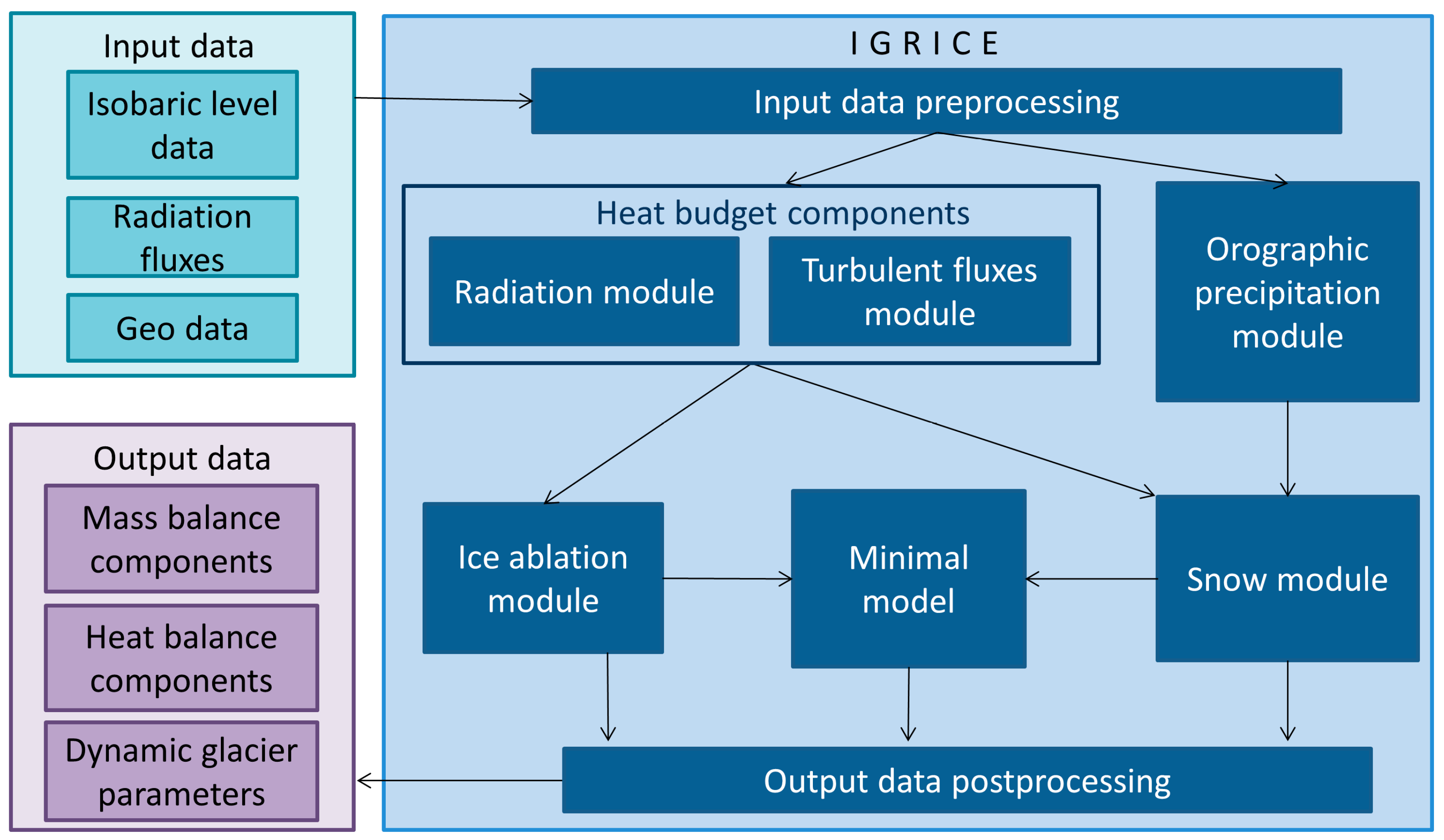
Figure 1. General scheme of the IGRICE model.
Climate 13 00248 g001
Figure 2. Satellite images of selected glaciers (a) in the Caucasus region (Garabashi and Dzhankuat, red contours) and (b) in Svalbard (Aldegonda and East Grønfjord, black contours). Insets depict larger regional views.
Climate 13 00248 g002
Figure 3. Monthly mean temperature (red line), precipitation (blue bars), and wind speed (gray line) for the period of 1984–2021 based on ERA5 reanalysis data for the (a,c,e,g) lowermost and (b,d,f,h) uppermost zones of the (a,b) Garabashi, (c,d) Dzhankuat, (e,f) Aldegonda, and (g,h) East Grønfjord glaciers.
Climate 13 00248 g003
Figure 4. Mass-balance components with altitude based on observations (black dashed line) and model results (red line) and their interannual variability based on modeling results (gray area) for the (a,b) Garabashi, (c,d) Dzhankuat, (e,f) Aldegonda, and (g,h) East Grønfjord glaciers.
Climate 13 00248 g004
Figure 5. Evolution of mass balance (in black), accumulation (in blue), and ablation (in red) according to modeling results (dashed lines) and observations (solid lines and points) for (a) Garabashi, (b) Dzhankuat, (c) Aldegonda, and (d) East Grønfjord glaciers.
Climate 13 00248 g005
Figure 6. Scatterplots for modeled and observed accumulation (left column), ablation (central column), and mass balance (right column) for the (ac) Garabashi, (df) Djankuat, (gi) Aldegonda, and (jl) East Grønfjord glaciers. Also shown are regression lines (solid lines) indicating the regression equation and correlation coefficient; the line of perfect fit is shown as a dashed line.
Climate 13 00248 g006
Figure 7. (a,b) Long-term mean (1984–2021) annual precipitation (mm) and snow depth (m w.e.) (in color and thin black contours) on (c,d) June 1 and (e,f) September 1 on Mt. Elbrus according to (a,c,e) modeling results and (b,d,f) ERA5-Land reanalysis. Thick black curves show Garabashi Glacier borders.
Climate 13 00248 g007
Figure 8. Evolution of glacier areas based on modeling results (solid lines) and observational data (points) for the Garabashi (blue), Djankuat (red), Aldegonda (green), and East Grønfjord (gray) glaciers.
Climate 13 00248 g008
Figure 9. Components of heat balance for the period of 1984–2021, calculated for the lowermost (left column) and uppermost (right column) zones of the (a,b) Garabashi, (c,d) Djankuat, (e,f) Aldegonda, and (g,h) East Grønfjord glaciers: net shortwave radiation balance (red), net longwave radiation balance (magenta), L W r o c k (green), sensible heat flux (orange), latent heat flux (blue), and heat available for ice melting (black).
Climate 13 00248 g009
Figure 10. Interannual variability of radiation balance anomalies, incoming shortwave and longwave flux anomalies, albedo, and cloudiness factor (CF) on the Caucasus glaciers: (a) Garabashi and (b) Djankuat. Dashed lines show linear trends.
Climate 13 00248 g010
Figure 11. Interannual variability of air temperature and specific humidity anomalies, fraction of liquid precipitation, and sensible heat flux on the Svalbard glaciers: (a) Aldegonda and (b) East Grønfjord. Dashed lines show linear trends.
Climate 13 00248 g011
Table 1. Main model parameters for each glacier.
Type of ParameterParameterGarabashiDjankuatAldegondaEast Grønfjord
Morphometric parameters *General convexity of topographyConvex ConcaveConcave Concave
Glacier length (m); volume (m3)5800; 2.8 × 1083400; 1.5 × 1083600; 3.9 × 1085300; 3.7 × 10⁸
Altitudinal zones, m asl3200/3500/3800/4100 /44002900/3200/3500200/400100/300
Area fraction of altitude zones0.05/0.15/0.4/0.25/0.150.2/0.4/0.40.7/0.30.3/0.7
Slope of altitude zones, °22.5/22.5/22.5/22.5/22.516/30/105/155/5
Glacier azimuth, °180300600
For dynamical block α m 3.3421.5
α 0.0030.00060.00060.0007
For precipitation blockLarge-scale slope in grid cell, °27271313
Maximal height in grid cell, m56003700700700
c d 0.250.50.50.5
Parameters controlling ablation/accumulationTemperature at the glacier bottom, °C−8−4−4−4
L W r o c k parametrization (for each zone)On/Off/Off /
Off/Off
On/On/OffOn/OffOn/Off
Slope of rocks, °27271313
Temperature of rocks, °C40402020
Debris on ice surface (for ice albedo parametrization)YesYesYesYes
Fraction of thin debris on surface in the lowest zone0.50.50.30.3
Shielding effect of debris coverOffOnOffOff
Fraction of thick debris cover in each zone-0.35/0.15/0.0--
Fraction of avalanche feeding, %51055
Snow concentration coefficient in each zone1/1/1.1/0.9/0.82.3/2.7/3.01.5/1.81.5/1.5
* For the starting year of experiments, i.e., 1983.
Table 2. Linear trends (per 10 years) of the main meteorological parameters for the considered glaciers (statistically significant trends are shown in bold). P—surface pressure, T a —near-surface air temperature.
GlacierMeteorological ParametersPrecipitation Rate, mm/day
P, hPa T a , °C q a , g kg−1 U , m s−1TotalLiquidSolid
Garabashi0.470.410.04−0.07−0.060.02−0.08
Djankuat0.400.410.04−0.04−0.27−0.05−0.23
Aldegonda−0.140.970.130.030.050.06−0.03
East Grønfjord−0.120.980.130.030.030.09−0.05
Table 3. Linear trends (per 10 years) of heat-balance components on the studied glaciers (statistically significant trends are shown in bold). S W n e t —net shortwave radiation balance, L W n e t —net longwave radiation balance on the surface.
Glacier S c ,
W m−2
D s ,
W m−2
A,
%
L W , W m−2 L W ,
W m−2
S W n e t ,
W m−2
L W n e t , W m−2H,
W m−2
LE,
W m−2
Garabashi1.98−1.52−10.891.041.59−0.070.600.08
Djankuat1.50−1.08−20.921.002.350.430.220.03
Aldegonda−0.12−0.63−23.634.060.51−0.310.600.05
East Grønfjord−0.12−0.70−23.504.230.59−0.620.48−0.1
Table 4. Pearson correlation coefficients (statistically significant in bold) between mass-balance components and various driving factors. Pliq—fraction of liquid precipitation.
AccumulationAblationMass Balance
GarabashiDjankuatAldegondaEast GrønfjordGarabashiDjankuatAldegondaEast GrønfjordGarabashiDjankuatAldegondaEast Grønfjord
P−0.22−0.370.080.010.610.760.060.07−0.57−0.69−0.04−0.06
T a −0.17−0.310.13−0.020.600.730.460.49−0.54−0.63−0.39−0.44
q a 0.21−0.050.05−0.120.380.530.650.67−0.24−0.36−0.56−0.62
P l i q −0.20−0.50−0.45−0.380.46−0.200.760.70−0.43−0.15−0.77−0.69
H0.00.30−0.04−0.040.400.400.460.34−0.32−0.09−0.42−0.31
LE−0.21−0.14−0.16−0.210.080.400.580.50−0.14−0.33−0.55−0.48
S W n e t −0.54−0.54−0.43−0.320.910.950.690.69−0.92−0.90−0.71−0.67
L W n e t 0.40−0.150.000.01−0.030.570.460.330.16−0.45−0.41−0.29
Disclaimer/Publisher’s Note: The statements, opinions and data contained in all publications are solely those of the individual author(s) and contributor(s) and not of MDPI and/or the editor(s). MDPI and/or the editor(s) disclaim responsibility for any injury to people or property resulting from any ideas, methods, instructions or products referred to in the content.