On the Unforced or Forced Nature of the Atlantic Multidecadal Oscillation: A Linear and Nonlinear Causality Analysis

Abstract

In recent years, there has been intense debate in the literature as to whether the Atlantic Multidecadal Oscillation (AMO) is a genuine representation of natural climate variability or is substantially driven by external factors. Here, we perform an analysis of the influence of external (natural and anthropogenic) forcings on the AMO behaviour by means of a linear Granger causality analysis and by a nonlinear extension of this method. Our results show that natural forcings do not have any causal role on AMO in both linear and nonlinear analyses. Instead, a certain influence of anthropogenic forcing is found in a linear framework.

1. Introduction

Recent global warming attribution studies have shown that the global temperature trend is substantially due to changes in the value of anthropogenic forcings, while its interannual or decadal variability is influenced by the natural variability modes of the climate system, the most impactful of which appears likely to be the El Niño Southern Oscillation (ENSO) [1,2].

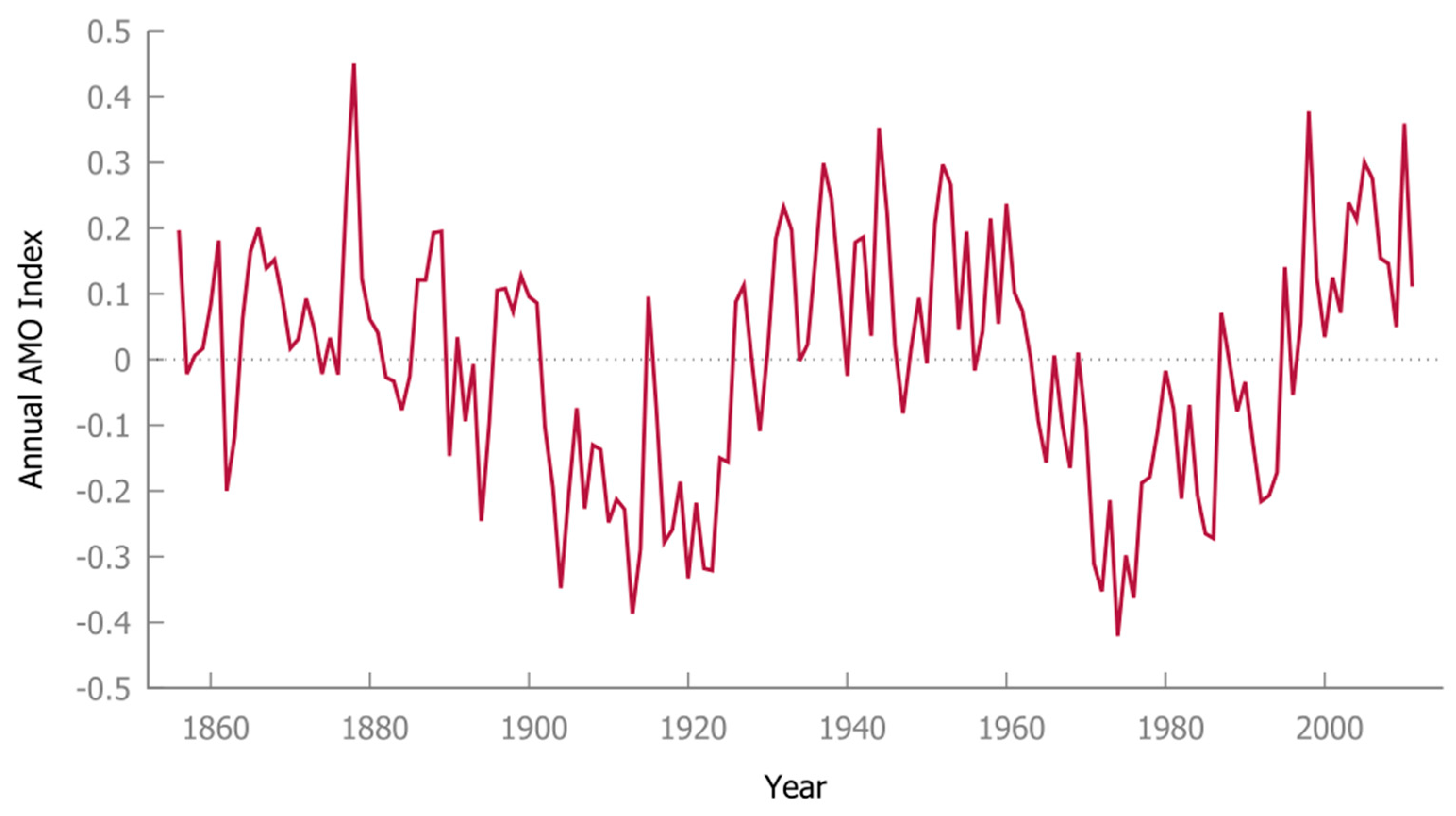
Although it is obviously being investigated what perturbative effects anthropogenic forcings may have on the course of these natural cycles (see, for instance, Chapter 3 of [1]), their typical behaviour is always ascribed to the natural dynamics of the climate system. Recently, however, this has been called into question with regard to the Atlantic Multidecadal Oscillation (AMO) (see Figure 1), a cycle in the Atlantic Ocean that influences climate and meteorological phenomena in several regions of the world: see, for instance, [3], for a recent example of these impacts.

Figure 1. The oscillating behaviour of AMO time series.

A good number of AMO “attribution” studies have been carried out in the past. Papers on this topic can be divided into two broad strands: those that claim a fundamental role for factors internal to climate dynamics (including ocean circulation) in driving the behaviour of the AMO time series and those that see external forcings, especially sulphate aerosols, as influential, particularly over the last century. Thus, is AMO a genuine representation of the internal natural variability of the climate system or is substantially driven by external factors? This issue is much debated and there is no consensus on the answer to the previous question in the scientific community.

In this framework, here, we employ data-driven methods for investigating this topic. After some preliminary applications to the study of the influences on AMO by other climate modes of internal variability, we focus on the possible driving roles of the external (natural or anthropogenic) forcings. In doing so, we present an analysis that can complement the past ones, performed almost exclusively through Global Climate Models (GCMs), and can contribute to the debate on AMO “attribution”.

Kushnir [4] was probably the first to analyse quasi-periodic variations in the North Atlantic on a multi-decadal scale, using about a century of temperature and pressure observations. Meanwhile, Schlesinger and Ramankutty [5], performing a spectral analysis of global surface air and sea temperature data, showed that the ~65-year oscillation is mainly the North Atlantic mode: it occurs only in this area. Thus, the term AMO implies not only the Atlantic origin of this oscillation but also its low-frequency character. Further details on the variability of low-frequency AMO have been described by Polonskii and Voskresenskaya [6].

But by what mechanism are these quasi-periodic AMO oscillations produced? The first clue was certainly the meridional heat transport (MHT) in the North Atlantic. However, there are different views on the main causes of AMO generation and some authors have shown that AMO could be generated without any active ocean dynamics.

It is clear that, in the complex geophysical system, different mechanisms can act simultaneously. Here, however, our aim is to analyse which single influences can be the driving factors for AMO.

To our knowledge, the studies that have faced this problem of AMO “attribution” were published in [7,8,9,10,11,12,13,14,15,16,17,18,19,20,21]. The first papers focused on the role of natural changes in oceanic circulation [7,8]. Then, volcanic forcings were considered as the main drivers of AMO [9] and a role for anthropogenic aerosol emissions came to be considered as very relevant for the twentieth century [10]. Zhang et al. [11] found discrepancies that cast doubts on previous claims in [10] but without any alternative explanation for the AMO behaviour.

Later, Knudsen et al. [12] suggested that the Atlantic Meridional Overturning Circulation (AMOC) could be crucial as a link between external forcing and North Atlantic sea-surface temperatures, a conjecture that is able to reconcile previous opposing theories concerning the origin of the AMO. Clement et al. [13] showed that AMO is forced by mid-latitude atmospheric circulation, while Bellucci et al. [14] studied the 1940–1975 North Atlantic cooling and found a key role for anthropogenic forcings in driving it. In the meantime, Cane et al. [15] showed that the ocean is influent on AMO, even if it seems not so important for the simulation of the surface temperature climate variability. Murphy et al. [16], via a modelling study, showed a clear role for external forcings in driving the observed AMO and argued that, very likely, internal variability is insufficient to drive the AMO multidecadal changes observed over the last century. A new paper, [17], promptly confirmed this latter result and showed that greenhouse gases (GHGs) and tropospheric aerosols were probably the main drivers of the AMO in the latter part of the twentieth century.

On contrast, other results [18,19,20] suggested internal sources for the AMO behaviour, e.g., oceanic variability and circulation. Finally, it should of course be noted that the AMO signal has been estimated for centuries and millennia well before the industrial era: see, for example, [22]. Therefore, it is clear that the above-mentioned studies may seem rather limited in establishing the unforced or forced nature of AMO. In this regard, however, a paper by Mann et al. [21] should be noted, where they addressed this issue and showed how, throughout the last millennium, this oscillation may be due to pulses of volcanic activity.

Here we stress again the different results found and that the vast majority of studies have been performed through dynamical analyses via GCMs. In this research framework, however, data-driven methods can contribute to analysing the problem via complementary approaches. This has been performed, for instance, in [23], where one of us (A.P.) applied a neural network tool [24] to this analysis, finding a clear role for anthropogenic forcings (especially sulphate aerosols) in driving AMO behaviour.

In any case, as already shown for global warming attribution studies, also other data-driven methods can be applied to analyse causality relationships in the climate system. See, for instance, some of our previous papers on this topic [25,26,27]. Thus, here we perform an analysis of the influence of external (natural and anthropogenic) forcings on the AMO behaviour by means of a linear Granger causality analysis and by a nonlinear extension of this method, with the aim of contributing to the scientific debate on this topic.

2. Methods

2.1. Granger Causality Analysis

Granger causality analysis is traditionally based on the specification of a Vector Autoregressive (VAR) model. However, this approach is adequate only when the interactions among time series are linear. Vice versa, if the dynamics are nonlinear, this approach might fail in interpreting dynamical interactions among processes, thus resulting in an erroneous interpretation of causal relations. Therefore, here we use both linear Granger causality tests and nonlinear causality ones.

2.1.1. Linear Granger Causality

The linear causality analysis is conducted using the Toda and Yamamoto (TY) procedure [28]. This procedure consists of the following steps.

Step 1. Determine the maximum order of integration m of the variables x and y.

Step 2. Determine the p order of the following VAR model for the variables x and y:

$$x_t=\alpha +\beta t+\sum _{i=1}^p{\alpha }_i{x}_{t-i}+\sum _{i=1}^p{\beta }_i{y}_{t-i}+u_{1t},$$

(1)

$$y_t=\alpha +\beta t+\sum _{i=1}^p{\gamma }_i{y}_{t-i}+\sum _{i=1}^p{\delta }_i{x}_{t-i}+u_{2t}.$$

(2)

This can be performed using one of the automatic criteria proposed in the literature (Akaike information criterion (AIC), Bayesian information criterion (BIC), Hannan–Quinn information criterion (HQC) among others).

Step 3. Estimate (using the least squares method) the following (augmented) VAR model:

$$x_t=\alpha +\beta t+\sum _{i=1}^{p+m}{\alpha }_i{x}_{t-i}+\sum _{i=1}^{p+m}{\beta }_i{y}_{t-i}+u_{1t},$$

(3)

$$y_t=\alpha +\beta t+\sum _{i=1}^{p+m}{\gamma }_i{y}_{t-i}+\sum _{i=1}^{p+m}{\delta }_i{x}_{t-i}+u_{2t}.$$

(4)

Step 4. Test the null hypothesis of non-causality from y to x:

$$H_0:{\beta }_1={\beta }_2=\cdots ={\beta }_p=0,$$

(5)

using the statistic F, which under H₀ is asymptotically distributed as a F with p and T − 2(p + m) − 2 degrees of freedom, where T is the number of observations used to estimate the VAR model. The F statistic is calculated using the following formula:

$$F=\frac{\left({RSS}_R-{RSS}_U\right)/p}{{RSS}_U/\left[T-2\left(p+m\right)-2\right]},$$

(6)

where with RSS_R we have indicated the sum of the squared residuals of the model (restricted)

$$x_t=\alpha +\beta t+\sum _{i=1}^{p+m}{\alpha }_i{x}_{t-i}+\sum _{i=p+1}^{p+m}{\beta }_i{y}_{t-i}+u_{1t}$$

(7)

and with RSS_U we denote the sum of the squared residuals of the model (unrestricted)

$$x_t=\alpha +\beta t+\sum _{i=1}^{p+m}{\alpha }_i{x}_{t-i}+\sum _{i=1}^{p+m}{\beta }_i{y}_{t-i}+u_{1t}.$$

(8)

If the F statistic is greater than the critical value, then we reject the null hypothesis and conclude that y causes x.

The TY procedure is used since it can be applied to any order of integration and does not depend on the cointegration properties of the system and thus permits avoiding any pre-test bias.

2.1.2. Nonlinear Granger Causality

In order to test for nonlinear Granger causality, we use a non-parametric method developed by Diks and Panchenko [29]. They developed a new nonparametric technique to apply for the residuals of a VAR model. The main idea behind applying the Diks–Panchenko (DP) test to the residuals of a VAR is to examine whether there are nonlinear causal relationships among the residuals of different variables within the VAR model. The residuals are delinearised and therefore we can ensure that the results of the non-parametric tests are based solely on the nonlinear nature of the variables. The test involves the following steps.

Step 1. Establish the lag length of the VAR model.

Step 2. Estimate the VAR model and save the residuals.

Step 3. Choose the values for lag lengths L_x and L_y and scale parameter ϵ. The meaning of these parameters is discussed in [29].

Step 4. Conduct the DP test using the residuals obtained from Step 2.

Following the convention in previous studies, eight values of lags: L_x = L_y = 1, 2, …, 8 and two scale parameters ϵ = 1 and ϵ = 1.5 were used.

3. Data Description

In this investigation, even for a consistent comparison with the previous paper by Pasini et al. [23], we consider annual data for the AMO index and the following radiative forcings: RFWARM, which is the warming part of the anthropogenic forcing (GHGs + BC RFs), its cooling part represented by sulphates (RFSOX), the RF of the solar activity (RFSOLAR) and the RF of volcanic emissions (RFVOL). In the following analysis, we also use the sums RFNAT (RFSOLAR + RFVOL), RFANTH (RFWARM + RFSOX) and RFTOT (RFNAT + RFANTH).

In this paper, we consider the AMO index calculated with a standard method [30]: its time series is freely available at www.esrl.noaa.gov/psd/data/timeseries/AMO (accessed on 1 March 2024). Data about the anthropogenic radiative forcings are downloaded from the dataset collected at http://www.sterndavidi.com/datasite.html (accessed on 1 March 2024, see also the paper by Stern and Kaufmann [31]). In the present paper, the data on GHG concentrations come from the NASA/GISS website and their RF calculations are performed through well-known formulas [32,33]. The global estimates of sulphate emissions in the past [34,35] and the computation of direct and indirect RFs as in [31]—which is based on slight modifications of previous studies [36,37]—supply us with data about the radiative forcing of sulphates. These last data are available until 2007: to consider a prolonged time series but without a too long extrapolation, we continue this series of RFSOX with constant data until 2011. Past data about the RF of black carbon come from the RCP8.5 scenario [38]. For data concerning natural radiative forcings, solar irradiance is approximated by an index previously assembled [39], and its data are downloadable from https://data.giss.nasa.gov/modelforce/solar.irradiance/ (accessed on 1 March 2024). The conversion from solar irradiance to RFSOLAR is obtained in a standard way [33]. Optical thickness data [40], available at https://data.giss.nasa.gov/modelforce/straaer/ (accessed on 1 March 2024), are considered as a proxy of the volcanic activity of dust emissions. RFVOL is set at 27 times the optical thickness [31].

As we will see below, before analysing the possible driving roles of external forcings on AMO, we carried out an analysis of the influences between other modes of natural variability and AMO itself. In doing so, we used the data series of the Atlantic Meridional Overturning Circulation (AMOC) and the North Atlantic Oscillation (NAO). These data were downloaded from https://erda.ku.dk/archives/cb78329f209d8ff2b4dd810abe4780ae/published-archive.html (accessed on 10 April 2024) and https://crudata.uea.ac.uk/cru/data/nao/ (accessed on 10 April 2024), respectively.

Preliminary Analysis

Preliminary to the Granger causality analysis, it is necessary to establish the order of integration of the involved time series. We remember that an integrated time series of order d, denoted as I(d), is a time series that have to be differenced d times to achieve stationarity.

To detect the order of integration of the variables, we use the Augmented Dickey–Fuller (ADF) test. To carry out the ADF tests, we estimate the following auxiliary regressions for each variable of interest y:

$$\Delta y_t={a+bt+cy}_{t-1}+c_1\Delta y_{t-1}+\cdots +c_k\Delta y_{t-k}+u_t,$$

(9)

where Δ is the first difference operator, u_t∼WN(0, σ²_u).

In this parametric framework, y_t is non-stationary (has a unit root) if c = 0. We test H₀: c = 0 against H₁: c < 0 using the test statistic

$${ADF}_t=\frac{\widehat{c}}{SE\left(\widehat{c}\right)},$$

(10)

where $\widehat{c}$ is the ordinary least square estimate of c and $SE\left(\widehat{c}\right)$ is its standard error. Under H₀: c = 0, this statistic follows asymptotically a Dickey–Fuller distribution. We reject H₀ if ADF_t is less than the critical value.

Applying the ADF test, we have obtained the following results: the series AMO, RFSOLAR, RFVOL, RFNAT, RFTOT are I(0), while the series RFSOX, RFWARM, RFANTH are I(1): see Table 1.

Table 1. Augmented Dickey–Fuller test. Estimated model: Δy_t = a + bt + cy_t−1 + c₁Δy_t−1 + … + c_kΔy_t−k + u_t.

Series	k	Null Hypothesis	Test Statistic ADFt	p-Value	Decision
AMO	0	c = 0	−5.42184	2.47 × 10−5	I(0)
RFSOX	1	c = 0	−1.031041	0.9382	I(1)
DRFRSOX *	0	c = 0	−7.70739	1.743 × 10−11	I(0)
RFWARM	1	c = 0	0.501236	0.9993	I(1)
DRFWARM *	0	c = 0	−5.9137	1.875 × 10−6	I(0)
RFHANT	1	c = 0	1.856	1.0000	I(1)
DRFHANT *	2	c = 0	0.501236	0.007485	I(0)
RFSOLAR	7	c = 0	−0.949026	0.949	I(1)
DRFSOLAR *	2	c = 0	−9.44782	1.263 × 10−17	I(0)
RFVOL	1	c = 0	−7.33584	2.508 × 10−10	I(0)
RFNAT	1	c = 0	−7.27811	3.75 × 10−10	I(0)
RFTOT	2	c = 0	−4.38025	0.002295	I(0)
AMOC	0	c = 0	−4.99828	0.0001821	I(0)
NAO	0	c = 0	−10.5005	7.564 × 10−22	I(0)

* D stands for the first difference of the series. The lag order k is automatically selected using BIC criterion, testing down from 12 lags. p-values are taken from [41].

4. Results

Although the main objective of this paper is to understand whether AMO is forced or unforced by external forcings, obviously a causality analysis between various modes of the natural variability of the coupled atmosphere–ocean system and AMO is of interest and is, as far as we know, a novelty when seen as an application of our methods.

Thus, referring to the data analysed in previous papers published in the literature, such as [42], we applied our methods to the study of influences from AMOC to AMO and from NAO to AMO. The results (not explicitly reported here but available on request) show that these natural variability modes have no causal role on AMO, as resulting from both the linear Granger analysis and the nonlinear Diks–Panchenko test.

Our results about the influences of external forcings on AMO give quite clear indications too. Firstly, natural forcings do not show any causal role on AMO in both linear and nonlinear analyses. The p-values are always very high, even in the case of the sum of RFSOLAR and RFVOL in RFNAT (see Table 2, Table 3, Table 4, Table 5, Table 6, Table 7, Table 8, Table 9 and Table 10), and the results are insensitive to choices of L_x, L_y and ϵ.

Table 2. Toda–Yamamoto Granger non-causality test ¹.

Null Hypothesis	Test Statistic	p-Value
RFSOLAR does not cause AMO	F(2, 146) = 0.36741	0.6932

¹ The p order of the VAR model has been determined using the BIC criterion.

Table 3. Nonlinear Granger causality test. Null hypothesis: RFSOLAR does not cause AMO. ϵ = 1.

Lx = Ly	Test Statistic	p-Value
1	−1.313	0.90545
2	−1.637	0.94916
3	−0.944	0.82740
4	−0.117	0.54674
5	−0.094	0.53750
6	0.413	0.33967
7	0.493	0.31117
8	−0.511	0.69545

Table 4. Nonlinear Granger causality test. Null hypothesis: RFSOLAR does not cause AMO. ϵ = 1.5.

Lx = Ly	Test Statistic	p-Value
1	−1.242	0.89282
2	−0.848	0.80165
3	−0.649	0.74181
4	−1.297	0.90268
5	−1.222	0.88911
6	−1.083	0.86066
7	−0.101	0.54038
8	−0.388	0.65108

Table 5. Toda–Yamamoto Granger non-causality test ¹.

Null Hypothesis	Test Statistic	p-Value
RFVOL does not cause AMO	F(1, 152) = 1.9506	0.1646

¹ The p order of the VAR model has been determined using the BIC criterion.

Table 6. Nonlinear Granger causality test. Null hypothesis: RFVOL does not cause AMO. ϵ = 1.

Lx = Ly	Test Statistic	p-Value
1	−0.977	0.83577
2	−0.804	0.78932
3	−0.157	0.56257
4	0.717	0.23673
5	0.971	0.16574
6	0.422	0.33647
7	0.359	0.35989
8	0.599	0.27474

Table 7. Nonlinear Granger causality test. Null hypothesis: RFVOL does not cause AMO. ϵ = 1.5.

Lx = Ly	Test Statistic	p-Value
1	−1.417	0.92177
2	−1.011	0.84404
3	−1.186	0.88226
4	−0.987	0.83816
5	0.763	0.22274
6	0.067	0.47328
7	0.398	0.34538
8	0.474	0.31781

Table 8. Toda–Yamamoto Granger non-causality test ¹.

Null Hypothesis	Test Statistic	p-Value
RFNAT does not cause AMO	F(1, 152) = 1.9519	0.1644

¹ The p order of the VAR model has been determined using the BIC criterion.

Table 9. Nonlinear Granger causality test. Null hypothesis: RFNAT does not cause AMO. ϵ = 1.

Lx = Ly	Test Statistic	p-Value
1	−0.621	0.73283
2	−1.349	0.91140
3	−0.372	0.64496
4	0.780	0.21762
5	0.999	0.15895
6	0.167	0.43370
7	0.306	0.37974
8	0.552	0.29049

Table 10. Nonlinear Granger causality test. Null hypothesis: RFNAT does not cause AMO. ϵ = 1.5.

Lx = Ly	Test Statistic	p-Value
1	−1.138	0.87254
2	−0.832	0.79722
3	−0.985	0.83775
4	−0.999	0.84106
5	0.699	0.24239
6	0.020	0.49195
7	0.406	0.34240
8	0.537	0.29572

On the other hand, in the case of anthropogenic forcings the p-values are generally smaller. However, RFSOX does not show a causal role on AMO (see Table 11, Table 12 and Table 13), while RFWARM does, at 5% significance in the linear case (see Table 14). In the nonlinear tests, RFWARM also does not show a causal effect, except in one case for L_x = L_y = 3 and epsilon equal to 1 (see Table 15 and Table 16). When RFWARM and RFSOX are summed up in RFANTH, the causality remains in the linear Granger causality (see Table 17), and this is even the case when considering the total forcing RFTOT (see Table 18). In the nonlinear tests, the null hypothesis of noncausality is always confirmed even in the latter cases.

Table 11. Toda–Yamamoto Granger non-causality test ¹.

Null Hypothesis	Test Statistic	p-Value
RFSOX does not cause AMO	F(2, 146) = 0.049969	0.9513

¹ The p order of the VAR model has been determined using the BIC criterion.

Table 12. Nonlinear Granger causality test. Null hypothesis: RFSOX does not cause AMO. ϵ = 1.

Lx = Ly	Test Statistic	p-Value
1	0.853	0.1967
2	−0.237	0.5935
3	−0.475	0.6826
4	−0.400	0.6555
5	0.507	0.3060
6	0.656	0.2557
7	0.162	0.3325
8	−0.634	0.7369

Table 13. Nonlinear Granger causality test. Null hypothesis: RFSOX does not cause AMO. ϵ = 1.5.

Lx = Ly	Test Statistic	p-Value
1	0.248	0.4019
2	−0.359	0.6402
3	0.122	0.4514
4	0.155	0.4382
5	0.541	0.2942
6	0.501	0.3083
7	0.433	0.3325
8	−0.372	0.6452

Table 14. Toda–Yamamoto Granger non-causality test ¹.

Null Hypothesis	Test Statistic	p-Value
RFWARM does not cause AMO	F(2, 146) = 3.9958	0.0204

¹ The p order of the VAR model has been determined using the BIC criterion.

Table 15. Nonlinear Granger causality test. Null hypothesis: RFWARM does not cause AMO. ϵ = 1.

Lx = Ly	Test Statistic	p-Value
1	0.910	0.18142
2	0.431	0.33310
3	1.692	0.04528
4	1.025	0.15266
5	0.996	0.15956
6	0.360	0.3594
7	0.176	0.43026
8	0.420	0.33741

Table 16. Nonlinear Granger causality test. Null hypothesis: RFWARM does not cause AMO. ϵ = 1.5.

Lx = Ly	Test Statistic	p-Value
1	0.040	0.48406
2	−0.226	0.58951
3	0.659	0.25501
4	0.068	0.47301
5	0.332	0.36990
6	−0.021	0.50852
7	−0.353	0.63804
8	0.289	0.38627

Table 17. Toda–Yamamoto Granger non-causality test ¹.

Null Hypothesis	Test Statistic	p-Value
RFANTH does not cause AMO	F(2, 146) =2.9199	0.0571

¹ The p order of the VAR model has been determined using the BIC criterion.

Table 18. Toda–Yamamoto Granger non-causality test ¹.

Null Hypothesis	Test Statistic	p-Value
RFTOT does not cause AMO	F(1, 152) = 3.9440	0.0488

¹ The p order of the VAR model has been determined using the BIC criterion.

How should we read these results in the framework of our previous knowledge and studies? Certainly, on the one hand, our work confirms the results of those previous studies, such as the only other data-driven investigation [23], which showed that anthropogenic forcings have a certain influence on AMO trends. On the other hand, it is not the influence of RFSOX that is important here but that of RFWARM. In both [23] and the present study, the negligible influence of natural forcings (and other modes of natural variability) and the importance of anthropogenic ones is confirmed, albeit in a different manner. Furthermore, whereas in [23] it was the nonlinear model that showed the influence of anthropogenic variables on AMO, here causality is found almost exclusively in Granger’s linear analysis.

5. Conclusions

The situation is therefore not definitely established and we cannot say that our results completely corroborate or totally refute those of previous studies. In any case, as shown in [43,44], research applying different and independent methods can make us realise how robust or not certain results are. Here, our contribution highlights a certain influence of anthropogenic forcing but with a different role than previously found. Furthermore, causality appears linear and not nonlinear.

What we can conclude is that our paper contributes to investigations into the nature of AMO, but further research into the role of these forcings on the AMO itself will need to be conducted to reach robust and shared results.

As a final remark, we would like to note that, sometimes, basing analysis solely on the observational data cannot fully separate natural climate variability and external forcings. Thus, a possible future development of our work could be the use of large ensemble simulations of climate models (as discussed in [45]) to further analyse our topic and compare new results with those obtained in this study.

References

- IPCC. Climate Change 2021: The Physical Science Basis. In Contribution of Working Group I to the Sixth Assessment Report of the Intergovernmental Panel on Climate Change; Masson-Delmotte, V., Zhai, P., Pirani, A., Connors, S.L., Péan, C., Berger, S., Caud, N., Chen, Y., Goldfarb, L., Gomis, M.I., et al., Eds.; Cambridge University Press: Cambridge, UK, 2021; 2391p. [Google Scholar]
- Timmermann, A.; An, S.I.; Kug, J.S.; Jin, F.F.; Cai, W.; Capotondi, A.; Cobb, K.M.; Lengaigne, M.; McPhaden, M.J.; Zhang, X.; et al. El Niño–Southern Oscillation complexity. Nature 2018, 559, 535–545. [Google Scholar] [CrossRef] [PubMed]
- Cai, Q.; Chen, W.; Chen, S.; Xie, S.-P.; Piao, J.; Ma, T.; Lan, X. Recent pronounced warming on the Mongolian Plateau boosted by internal climate variability. Nat. Geosci. 2024, 17, 181–188. [Google Scholar] [CrossRef]
- Kushnir, Y. Interdecadal Variations in North Atlantic Sea Surface Temperature and Associated Atmospheric Conditions. J. Clim. 1994, 7, 141–157. [Google Scholar] [CrossRef]
- Schlesinger, M.E.; Ramankutty, N. An oscillation in the global climate system of period 65–70 years. Nature 1994, 367, 723–726. [Google Scholar] [CrossRef]
- Polonskii, A.B.; Voskresenskaya, E.N. On the Statistical Structure of Hydrometeorological Fields in the North Atlantic. Phys. Oceanogr. 2004, 14, 15–26. [Google Scholar] [CrossRef]
- Knight, J.R.; Allan, R.J.; Folland, C.K.; Vellinga, M.; Mann, M.E. A signature of persistent natural thermohaline circulation cycles in observed climate. Geophys. Res. Lett. 2005, 32, L20708. [Google Scholar] [CrossRef]
- Jungclaus, J.; Haak, H.; Latif, M.; Mikolajewicz, U. Arctic-North Atlantic interactions and multidecadal variability of the meridional overturning circulation. J. Clim. 2005, 18, 4013–4031. [Google Scholar] [CrossRef]
- Otterå, O.H.; Bentsen, M.; Drange, H.; Suo, L. External forcing as a metronome for Atlantic multidecadal variability. Nat. Geosci. 2010, 3, 688–694. [Google Scholar] [CrossRef]
- Booth, B.B.B.; Dunstone, N.J.; Halloran, P.R.; Andrews, T.; Bellouin, N. Aerosols implicated as a primer driver of twentieth-century North Atlantic climate variability. Nature 2012, 484, 228–232. [Google Scholar] [CrossRef]
- Zhang, R.; Delworth, T.L.; Sutton, R.; Hodson, D.L.; Dixon, K.W.; Held, I.M.; Kushnir, Y.; Marshall, J.; Ming, J.; Vecchi, G.; et al. Have aerosols caused the observed Atlantic multidecadal variability? J. Atmos. Sci. 2013, 70, 1135–1144. [Google Scholar] [CrossRef]
- Knudsen, M.F.; Jacobsen, B.H.; Seidenkrantz, M.-S.; Olsen, J. Evidence for external forcing of the Atlantic Multidecadal Oscillation since termination of the little ice age. Nat. Commun. 2014, 5, 3323. [Google Scholar] [CrossRef] [PubMed]
- Clement, A.C.; Bellomo, K.; Murphy, L.N.; Cane, M.A.; Mauritsen, T.; Rädel, G.; Stevens, B. The Atlantic Multidecadal Oscillation without a role for ocean circulation. Science 2015, 350, 320–324. [Google Scholar] [CrossRef]
- Bellucci, A.; Mariotti, A.; Gualdi, S. The role of forcings in the twentieth-century North Atlantic multidecadal variability: The 1940–1975 North Atlantic cooling case study. J. Clim. 2017, 30, 7317–7337. [Google Scholar] [CrossRef]
- Cane, M.A.; Clement, A.C.; Murphy, L.N.; Bellomo, K. Low-pass filtering, heat flux, and Atlantic multidecadal variability. J. Clim. 2017, 30, 7529–7553. [Google Scholar] [CrossRef]
- Murphy, L.N.; Bellomo, K.; Cane, M.A.; Clement, A.C. The role of historical forcings in simulating the observed Atlantic Multidecadal Oscillation. Geophys. Res. Lett. 2017, 44, 2472–2480. [Google Scholar] [CrossRef]
- Bellomo, K.; Murphy, L.N.; Cane, M.A.; Clement, A.C.; Polvani, L.M. Historical forcings as main drivers of the Atlantic multidecadal variability in the CESM large ensemble. Clim. Dyn. 2018, 50, 3687–3698. [Google Scholar] [CrossRef]
- Kim, W.M.; Yeager, S.G.; Danabasoglu, G. Key role of internal ocean dynamics in Atlantic multidecadal variability during the last half century. Geophys. Res. Lett. 2018, 45, 13449–13457. [Google Scholar] [CrossRef]
- O’Reilly, C.H.; Zanna, L.; Woollings, T. Assessing external and internal sources of Atlantic multidecadal variability using models, proxy data, and early instrumental indices. J. Clim. 2019, 32, 7727–7745. [Google Scholar] [CrossRef]
- Athanasiadis, P.J.; Yeager, S.; Kwon, Y.O.; Bellucci, A.; Smith, D.W.; Tibaldi, S. Decadal predictability of North Atlantic blocking and the NAO. NPJ Clim. Atmos. Sci. 2020, 3, 20. [Google Scholar] [CrossRef]
- Mann, M.E.; Steinman, B.A.; Brouillette, D.J.; Miller, S.K. Multidecadal climate oscillations during the past millennium driven by volcanic forcing. Science 2021, 371, 1014–1019. [Google Scholar] [CrossRef]
- Knudsen, M.F.; Seidenkrantz, M.-S.; Jacobsen, B.H.; Kuijpers, A. Tracking the Atlantic multidecadal oscillation through the last 8000 years. Nat. Comm. 2011, 2, 178. [Google Scholar] [CrossRef]
- Pasini, A.; Amendola, S.; Federbusch, E. Is natural variability really natural? The case of Atlantic Multidecadal Oscillation investigated by a neural network model. Theor. Appl. Clim. 2022, 150, 881–892. [Google Scholar] [CrossRef]
- Pasini, A. Artificial neural networks for small dataset analysis. J. Thorac. Dis. 2015, 7, 953–960. [Google Scholar]
- Attanasio, A.; Pasini, A.; Triacca, U. A contribution to attribution of recent global warming by out-of-sample Granger causality analysis. Atmos. Sci. Lett. 2012, 13, 67–72. [Google Scholar] [CrossRef]
- Pasini, A.; Triacca, U.; Attanasio, A. Evidence of recent causal decoupling between solar radiation and global temperature. Environ. Res. Lett. 2012, 7, 034020. [Google Scholar] [CrossRef]
- Triacca, U.; Attanasio, A.; Pasini, A. Anthropogenic global warming hypothesis: Testing its robustness by Granger causality analysis. Environmetrics 2013, 24, 260–268. [Google Scholar] [CrossRef]
- Toda, H.Y.; Yamamoto, T. Statistical inference in Vector Autoregressions with possibly integrated processes. J. Econom. 1995, 66, 225–250. [Google Scholar] [CrossRef]
- Diks, C.; Panchenko, V. A new statistic and practical guidelines for nonparametric Granger causality testing. J. Econ. Dyn. Control 2006, 30, 1647–1669. [Google Scholar] [CrossRef]
- Enfield, D.B.; Mestas-Nunez, A.M.; Trimble, P.J. The Atlantic Multidecadal Oscillation and its relation to rainfall and river flows in the continental US. Geophys. Res. Lett. 2001, 28, 2077–2080. [Google Scholar] [CrossRef]
- Stern, D.I.; Kaufmann, R.K. Anthropogenic and natural causes of climate change. Clim. Chang. 2014, 122, 257–269. [Google Scholar] [CrossRef]
- Ramaswamy, V.; Boucher, O.; Haigh, J.; Hauglustaine, D.; Haywood, J.; Myhre, G.; Nakajima, T.; Shi, G.Y.; Solomon, S. Radiative Forcing of Climate Change. In Climate Change 2001: The Scientific Basis; Houghton, J.T., Ding, Y., Griggs, D.J., Noguer, M., van der Linden, P.J., Dai, X., Maskell, K., Johnson, C.A., Eds.; Cambridge University Press: Cambridge, UK, 2001; pp. 349–416. [Google Scholar]
- Kattenberg, A.; Giorgi, F.; Grassl, H.; Meehl, G.A.; Mitchell, J.F.B.; Stouffer, R.J.; Wigley, T.M.L. Climate Models-Projections of Future Climate. In Climate Change 1995: The Science of Climate Change; Houghton, J.T., Meira Filho, L.G., Callander, B.A., Harris, N., Kattenberg, A., Maskell, K., Eds.; Cambridge University Press: Cambridge, UK, 1996; pp. 285–357. [Google Scholar]
- Smith, S.J.; van Aardenne, J.; Klimont, Z.; Andres, R.J.; Volke, A.; Arias, S.D. Anthropogenic sulfur dioxide emissions: 1850–2005. Atmos. Chem. Phys. 2011, 11, 1101–1116. [Google Scholar] [CrossRef]
- Klimont, Z.; Smith, S.J.; Cofala, J. The last decade of global anthropogenic sulfur dioxide: 2000–2011 emissions. Environ. Res. Lett. 2013, 8, 014003. [Google Scholar] [CrossRef]
- Wigley, T.M.L.; Raper, S.C.B. Implications for climate and sea level of revised IPCC emissions scenarios. Nature 1992, 357, 293–300. [Google Scholar] [CrossRef]
- Boucher, O.; Pham, M. History of sulfate aerosol radiative forcings. Geophys. Res. Lett. 2002, 29, 22-1–22-4. [Google Scholar] [CrossRef]
- Meinshausen, M.; Smith, S.J.; Calvin, K.; Daniel, J.S.; Kainuma, M.L.; Lamarque, J.F.; van Vuuren, D.P. The RCP GHG concentrations and their extension from 1765 to 2300. Clim. Chang. 2011, 109, 213–241. [Google Scholar] [CrossRef]
- Lean, J. Evolution of the sun’s spectral irradiance since the Maunder Minimum. Geophys. Res. Lett. 2000, 27, 2425–2428. [Google Scholar] [CrossRef]
- Sato, M.; Hansen, J.E.; McCormick, M.P.; Pollack, J.B. Stratospheric aerosol optical depth, 1850–1990. J. Geophys. Res. 1993, 98, 22987–22994. [Google Scholar] [CrossRef]
- MacKinnon, J.G. Numerical distribution functions for unit root and cointegration tests. J. Appl. Econom. 1996, 6, 601–618. [Google Scholar] [CrossRef]
- McCarthy, G.D.; Haigh, I.D.; Hirschi, J.J.-M.; Grist, J.P.; Smeed, D.A. Ocean impact on decadal Atlantic climate variability revealed by sea-level observations. Nature 2015, 521, 508–510. [Google Scholar] [CrossRef] [PubMed]
- Pasini, A.; Mazzocchi, F. A multi-approach strategy in climate attribution studies: Is it possible to apply a robustness framework? Environ. Sci. Policy 2015, 50, 191–199. [Google Scholar] [CrossRef]
- Mazzocchi, F.; Pasini, A. Climate model pluralism beyond dynamical ensembles. WIREs Clim. Change 2017, 8, e477. [Google Scholar] [CrossRef]
- Deser, C.; Knutti, R.; Solomon, S.; Phillips, A.S. Communication of the role of natural variability in future North American climate. Nat. Clim. Chang. 2012, 2, 775–779. [Google Scholar] [CrossRef]
Disclaimer/Publisher’s Note: The statements, opinions and data contained in all publications are solely those of the individual author(s) and contributor(s) and not of MDPI and/or the editor(s). MDPI and/or the editor(s) disclaim responsibility for any injury to people or property resulting from any ideas, methods, instructions or products referred to in the content. |
© 2024 by the authors. Licensee MDPI, Basel, Switzerland. This article is an open access article distributed under the terms and conditions of the Creative Commons Attribution (CC BY) license (https://creativecommons.org/licenses/by/4.0/).