Article

Estimation and Validation of Snowmelt Runoff Using Degree Day Method in Northwestern Himalayas

by
Sunita
1,
Vishakha Sood
2,*,
Sartajvir Singh
3,
Pardeep Kumar Gupta
4,
Hemendra Singh Gusain
5,
Reet Kamal Tiwari
2,
Varun Khajuria
6 and
Daljit Singh
7
1
Department of Civil Engineering, Punjabi University, Patiala 147002, India
2
Department of Civil Engineering, Indian Institute of Technology, Ropar 140001, India
3
University Institute of Engineering, Chandigarh University, Mohali 140413, India
4
Department of Civil Engineering, Punjab Engineering College (Deemed to be University), Chandigarh 160012, India
5
Institute of Technology Management (DRDO), Mussoorie 248179, India
6
Department of Earth Sciences, University of Pisa, 56126 Pisa, Italy
7
Sant Longowal Institute of Engineering & Technology, Sangrur 148106, India
*
Author to whom correspondence should be addressed.
Climate 2024, 12(12), 200; https://doi.org/10.3390/cli12120200
Submission received: 23 September 2024 / Revised: 23 November 2024 / Accepted: 25 November 2024 / Published: 26 November 2024

Abstract

The rivers of the Himalayas heavily rely on the abundance of snow, which serves as a vital source of water to South Asian countries. However, its impact on the hydrological system of the region is mainly felt during the spring season. The melting of snow and consequent base flow significantly contribute to the incoming streamflow. This article examines the evaluation of the proportionate contribution to the total streamflow of Beas River up to Pandoh Dam through the snow melt. To analyze the snow melt, the snowmelt runoff model (SRM) has been utilized via dividing the study area into seven different elevation zones within a range of 853–6582 m and computing the percentage of snow cover, ranging from 15% to 90% across the basin. To validate the accuracy of the model, several metrics, such as coefficient of determination (R2) and volume difference (VD), are utilized. The R2 reveals that over the span of ten years, the daily discharge simulations exhibited efficiency levels ranging from 0.704 to 0.795, with VD falling within the range of 1.47% to 20.68%. This study has revealed that a significant amount of streamflow originates during the summer and monsoon periods, with snowmelt ranging from 10% to 45%. This research provides crucial understanding of the impact of snowmelt on streamflow, supplying essential knowledge on freshwater supply in the area.

1. Introduction

The significant increase in urbanization and population growth in the Himalayan region has resulted in a heightened demand for freshwater, underscoring the critical necessity for precise forecasts of glacier melting to anticipate stream flow. This unique environment, defined by its fragile ecosystem and challenging landscape, is vulnerable to frequent calamities such as landslides and flash floods. The glaciers of the Himalayas not only hold immense importance in regulating water flow in mountainous areas but also have a vital role in supporting the diverse ecological life of South and Central Asia with their abundant water resources [1,2]. The Himalaya mountain range is a vital supplier of freshwater and sustains approximately 60% of India’s population and other South Asian countries [3,4,5]. According to numerous climate change assessments, the current and past climate conditions have greatly affected the hydrological processes of snow and glaciers. This has led to increased runoff from snow and glaciers in the Himalayas to a considerable extent [5,6]. The authors of [7] conducted a thorough investigation on the Baspa River in the western Himalaya and uncovered a concerning decrease in glacier mass and runoff caused by rising temperatures. This aligns with previous findings from climate projections using global circulation models/regional climate models (GCMs/RCMs), which estimate a temperature increase of 1 °C to 2.5 °C in the Himalayan region since the twentieth century [8,9,10]. Many researchers have extensively documented the detrimental impact of amplified temperature rise on the Himalayan region. Such repercussions include glacial recession, heightened frequency of extreme occurrences, alterations in the ratio of snowfall to rainfall, and devastating flash floods [7,9].
According to some studies [11,12], the impact of climate change on the Himalayan glaciers has led to a decrease in biodiversity of endemic species and a change in ecosystem boundaries, resulting in challenges for agricultural production. With rising temperatures, particularly in high-elevation areas, the Himalayan forests are undergoing distribution pattern shifts and may also face modifications in their forest cover boundaries [11]. The warming temperature has the potential to significantly impact the amount of snow water equivalent (SWE) and the rate of snowmelt, posing a grave danger to the water reserves, agricultural production, and drinking water supply in the Himalayan region, according to previous studies [13,14,15,16,17]. Despite this potential threat, there is a lack of comprehensive research on the effects of climate change on snowmelt in the Himalayas [18,19,20,21,22,23,24,25].
Several research studies have indicated that, for modeling snowmelt runoff, the energy balance approach might outperform the temperature index model (TIM) based on the degree-day approach (DDA) [26,27,28]. However, the authors of [29,30] conducted comparisons between the modified TIM, which considers radiation and elevation bands, and the energy balance model for snowmelt computation. They found that the modified TIM exhibited superior performance compared to the energy balance model. This modified TIM has been found to be superior in the calculation of snowmelt by multiple studies [31,32,33]. Overall, the optimal approach for snowmelt runoff modeling is still a topic of ongoing research and debate. The application of the energy balance model has posed challenges in accurately computing snow hydrology in the Himalayas. This is due to its reliance on a significant level of precision and a large volume of data inputs, which are often unavailable [29,34].
Many hydrological models have been put in place to explain the runoff within a certain catchment area. However, these models have not been able to give estimates that are very accurate because of the absence of field data [35]. To overcome this issue, remote sensing and geographic information systems (GISs) were introduced. These technologies utilize remotely sensed data from sensors to gather information about the specific area of interest. An essential aspect of hydrological models is precipitation, but inaccessible areas with no rain gauges have made it challenging to accurately calculate these data. As a solution, satellites are used to estimate precipitation, but the results are not always precise [35].
Snow cover imagery can be accessed remotely through various satellites [36]. In this research, Moderate Resolution Imaging Spectroradiometer (MODIS) satellite imagery was utilized. To achieve the most accurate results, it is crucial to consider cloud and shadow conditions. To ensure the highest quality, it is advised to utilize images without any cloud interference. The functionality of the hydrological process heavily relies on the characteristics of the catchment area, which can be obtained using GIS techniques such as slope, aspect, area, and elevation [37]. With the advancement of remote sensing and GIS technologies, we are now able to calculate additional factors such as albedo [38], skin temperature [39], sunshine hours, and evapotranspiration [40]. According to various research studies [41,42,43], the application of the SRM has been proven effective in accurately simulating runoff in various Himalayan river basins. In this study, replication of the daily streamflow for the upper Beas River up to the Pandoh Dam using the snowmelt runoff model (SRM) and datasets derived from remote sensing was pursued. Therefore, the major objective of the study is estimation of snow melt of Beas River up to Pandoh Dam using the SRM from 2013–2022. This study presents a valuable database that can aid in the planning of hydropower projects in the Beas River and serve as a fundamental source of information for land and water resource management in the upper Beas basin.

2. Materials and Methods

2.1. Study Area

Figure 1 showcases the Beas River, a significant waterway in the vast Indus system that flows through the northern and western regions of India. This magnificent river stretches across two Indian states, Himachal Pradesh and Punjab, encompassing the far western segment of the Himalayas. Beginning at the Beas Kund in the Himalayas, it carves through the heart of Himachal Pradesh, covering 470 km before joining the Sutlej River in Punjab [44]. The Beas drainage basin envelopes a vast expanse of 20,303 square km. The Beas River, spanning approximately 116 km before reaching the Pandoh Dam, is the primary focus of this study. The segment of the river up to the dam has been divided into 7 elevation zones, and include (a) Advanced Spaceborne Thermal Emission and Reflection Radiometer (ASTER) global digital elevation model (GDEM), (b) slope image, (c) aspect image as depicted in Figure 2. The determined catchment area for the analysis spans 5384 square km and encompasses the region from Manali to Pandoh, with coordinates ranging from 31 ° 60′ N to 32 ° 43′ N and 77 ° 04′ E to 77 ° 74′ E. The Beas River is surrounded by multiple contributing streams, the most noteworthy being the Parbati and Sainj Khad. These glacier-fed tributaries converge with the Beas River at Bhuntar and Larji, respectively. Other significant tributaries, such as the Tirthan and Sainj, also meet near Larji, while the Bakhli Khad and Luni join the Beas River by Pandoh.
Figure 2 shows eight different systems (N, NE, E, SE, S, SW, W, NW) that were used in creating the aspect maps as the aspect of an inclined face greatly influences the shape of its topography. These maps provide a comprehensive overview of the direction of each land area. To establish the perspective for the study region, ASTER-GDEM was utilized, which resulted in a guide that incorporates slope and aspects from all four directions: northeast, southeast, northwest, and southwest.
Table 1 splits the region into seven elevation zones ranging from 853 to 6582 m. Zone 1, with elevations between 853 and 1600 m, covers 414.21 km2, which is 7.69% of the total area, and has an average elevation of 1359.8 m. Zone 2, ranging from 1600 to 2300 m, is larger, covering 1149.10 km2 (21.34% of the area) with an average elevation of 2031.9 m. Zone 3, from 2300 to 3100 m, covers 1219.34 km2 (22.64%) and has an average elevation of 2749.5 m. Zone 4, with elevations from 3100 to 3900 m, covers 908.54 km2 (16.87%) and averages 3518.6 m in elevation. Zone 5, from 3900 to 4600 m, spans 1107.57 km2 (20.57%) with an average elevation of 4310.6 m. Zone 6, covering elevations from 4600 to 5400 m, has an area of 571.47 km2 (10.64%) and an average elevation of 5016.7 m. Finally, Zone 7, the highest, ranges from 5400 to 6582 m, covering the smallest area of 13.46 km2 (0.25%) with an average elevation of 5608.7 m.

2.2. Dataset

To accurately simulate hydrological processes, the most crucial dataset to obtain is the meteorological parameters specific to the basin. For this study, daily precipitation data were utilized for the region from the India Meteorological Department: 0.25° × 0.25° high-resolution gridded data. To further enhance understanding, data from BBMB on other meteorological factors such as the maximum and minimum daily temperatures (Tmax and Tmin) were gathered.

2.2.1. Meteorological and Hydrological Data

In regions where snowmelt plays a major role, securing high-quality, evenly distributed, and adequate meteorological stations is a formidable task. These stations are often clustered in main valleys, necessitating the use of extrapolated data. Within snowmelt models, air temperatures serve dual functions: differentiating between rain and snow precipitation using threshold temperatures and determining crucial temperatures that influence the rate of snowmelt. Of all the parameters crucial to snowmelt modeling, temperature and rainfall play pivotal roles, with temperature indexing being a critical aspect of the SRM. This model utilizes extrapolated temperature data, obtained through the discussed methodology, which involves adjusting any negative values to zero before integrating them into the SRM. These extrapolated temperature data, gathered from temperature stations, and averaged for a ten-year span (2013–2022), are crucial in determining the hypsometric mean elevation. One of the main obstacles in hydrology is the difficulty in extending rainfall data from specific point stations to encompass entire basins. To tackle this concern, Bhadra and colleagues (2015) utilized ArcGIS technology to examine rainfall data from India Meteorological Department (IMD) grids. They then transformed these data into zonal rainfall, creating a comprehensive picture of rainfall patterns over a period of ten years (2013–2022) to incorporate into their model. In this study we addressed this challenge by extrapolating limited point-based data. We understand that this approach introduces some degree of uncertainty but it provides a practical solution in data-scarce regions like the rugged Himalayan area. To enhance the reliability of the model, we carefully selected representative meteorological stations and validated the model’s performance using metrics such as coefficient of determination (R2) and volume difference (VD). These metrics demonstrated consistent accuracy over the study period, reinforcing the robustness of our approach despite the data constraints.
Obtaining streamflow data for the study area was a crucial step in the research, where focus was on the dataset from 2013–2022. The data were collected on daily basis from Bhakra Beas Management Board (BBMB).

2.2.2. Topography and Snow Cover Dataset by Remote Sensing

At the heart of every hydrological model lies the digital elevation model (DEM), a crucial tool that unveils the intricate geographic features of a designated region. At its core, the DEM is a grid that maps out the unique elevation of each pixel in each area. Working within the powerful platform of ArcGIS, the DEM serves a multitude of purposes, from delineating catchment boundaries to classifying elevation zones, generating stream networks, and computing catchment characteristics like slope and aspect. In this study, the data were leveraged from the Shuttle Radar Topography Mission to obtain a high-resolution DEM of 30 m (ASTER-DEM 30 m), depicted in Figure 2.
In this study, advanced MODIS images were employed to accurately determine the extent of snow cover. MODIS data were selected for this study due to their global availability, high temporal resolution, and proven applicability in snow cover monitoring, especially in data-scarce mountainous regions. To mitigate the limitations of cloud cover, we applied standard cloud removal techniques and carefully validated the snow cover estimates against available ground data and observed streamflow. While these adjustments help reduce some uncertainties, we agree that inherent limitations persist and may affect the precision of SCA data. This dataset minimizes the overestimation typical of MODIS sensors by combining Terra and Aqua MODIS snow cover data. This approach addresses a significant weakness in Terra and Aqua MODIS 8-day composite C6 products, which previously exhibited a 46% overestimation and 3.66% underestimation, largely due to sensor limitations and cloud cover, respectively. Table 2 depicts the various datasets used.

2.3. Methodology

In 1975, Martinec introduced a temperature-based index model known as the snowmelt runoff model (SRM), which was utilized in smaller catchments throughout Europe. Referencing Figure 3, the SRM precisely mimics the contributions of both snowmelt and rainfall from mountainous regions, in combination with streamflow at the outlet point. To successfully generate streamflow from such catchments, it is essential to determine input variables derived from both rainfall and snowmelt. This distributed model accurately accounts for crucial hydrological processes, and thus, catchments were intentionally divided into distinct elevation zones to better analyze and simulate runoff streamflow. The study opted for the SRM for several reasons. Firstly, the SRM’s effectiveness lies in its heavy dependence on snow cover extent, requiring minimal data input, with the area covered by snow being determinable via satellite, aircraft, or ground measurements. Secondly, according to a study (WMO 1986) comparing different models, the SRM emerged as the most superior among them (WMO, 1986). The SRM is user-friendly and can be adapted to different climatic and geographical conditions with relatively few parameters. This makes it a practical tool for hydrologists and water resource managers [45]. SRM can integrate remote sensing data, such as satellite images, to monitor snow cover, which enhances the accuracy of runoff predictions. This capability is crucial for real-time water resource management [46]. The SRM provides valuable information for managing water resources, particularly in regions where snowmelt is a critical water source. It helps in planning for irrigation, hydropower, and flood control [47].
Throughout each time interval, the snowmelt runoff model performs three essential tasks. First, it extends meteorological data to various elevation zones. Next, it calculates the snowmelt rate for that interval. Finally, it combines the snowmelt runoff in the snow cover area (SCA) and rainfall runoff in the snow-free area (SFA) and compares it to the observed runoff. This model is designed to optimize the parameters used to route snowmelt runoff, while also taking into consideration the seasonal lapse rate of air temperature. The flow chart in Figure 3 provides a visual representation of the sequential steps within the model. Furthermore, the model incorporates the estimation of snow cover area (SCA) from the MODIS snow product to enhance its accuracy. Dividing the basin into different elevation zones, the SRM requires temperature, precipitation (in the form of rain or snow), and SCA to be given as input for each zone. Each day, the model processes the runoff from snowmelt and precipitation, then overlays it on the estimated flow during recession, ultimately transforming it into daily discharge from the catchment area. This approach has proven to be highly effective, showcasing the efficiency of the SRM in snowmelt modeling. The SRM by Martinec and Rango (1986) is shown as Equation (1):
Q + 1 = C · a T + T S + C R P × A × 10,000 86,400 × 1 K + 1 + Q K + 1
Equation (1) provided the calculation of average daily discharge (Q) [m3 s −1]. The equation includes several variables, including the runoff coefficient (C), which expresses the losses as a ratio of runoff to precipitation. The runoff coefficient distinguishes between snowmelt (Cₛ) and rain (CR) runoff. Another variable, an, represents the degree-day factor [cm °C−1d−1] that indicates the snowmelt depth resulting from one degree-day. The adjustment by temperature lapse rate (ΔT) corrects for temperature differences between the station and the average hypsometric elevation of the basin or zone [°C d]. The ratio of the snow-covered area to the total area (S) and the precipitation contributing to runoff (P) [cm] are also included in the equation. A preselected threshold temperature, T_CRIT, determines whether precipitation is rainfall and immediate or snow that is kept in storage until melting conditions occur. The area of the basin or zone (A) [km2], the recession coefficient (k), which indicates the decline of discharge in a period without snowmelt or rainfall, and the sequence of days during the discharge computation period (n) are also included in the equation. The variable m represents the sequence of days during a true recession flow period. The decision to use the degree-day method in this study stems from its simplicity, robustness, and widespread application in snowmelt modeling, particularly in data-sparse regions like the Himalayan basin. The method requires only temperature and snow cover area data, making it practical for regions where detailed meteorological data on radiation, wind, and humidity are often unavailable or difficult to obtain. While we acknowledge that DDA simplifies snowmelt as a linear function of temperature, it has been validated in numerous studies and shown to perform reliably for seasonal and annual runoff predictions, especially over extended temporal scales.

3. Results

3.1. Basin Characteristics

To extract the study area, the image underwent processing using Earth Resources Data Analysis System (ERDAS) Imagine 9.1 software. The study area was delineated by overlaying the vector layer onto the image. The basin was divided into seven distinct elevation zones, as shown in Figure 4. Using ArcGIS 10.6, a range of features were investigated within the basin, such as its size, elevation, and aspect (as shown in Figure 2). Area and elevation demonstrate that most of the basin falls within mid-elevation regions, with only a small portion occupying higher zones. This coincides with the recorded elevation where snow accumulation begins, which is 4800 m as indicated in Table 1.
The aspect of an inclined face greatly influences the shape of its topography. To accurately depict this factor, eight different systems (N, NE, E, SE, S, SW, W, NW) were used in creating the aspect maps. These maps provide a comprehensive overview of the direction of each land area. To establish the perspective for study region, the ASTER-GDEM was utilized, which resulted in a guide that incorporates aspects from all four directions: northeast, southeast, northwest, and southwest.

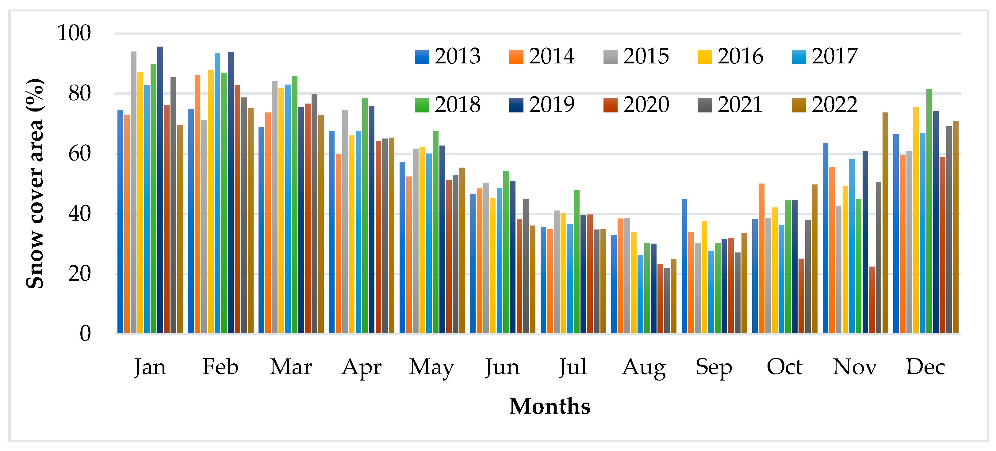
3.2. Snow Cover Area (SCA)

Improved MODIS data were used to calculate SCA between January 2013 and December 2022, following the methods outlined by [48,49]. The MODIS data are 8-day products and, to adapt these 8-day snow cover data for the snowmelt runoff model (SRM), which requires daily snow cover inputs, we have used extrapolation. This approach allows us to project the 8-day data forward, estimating snow cover for each day within the period to align with the SRM’s daily time step. Figure 5 showcases the snow-covered area maps for various months, revealing that the most substantial snow buildup typically occurs in January and February each year. Across different dates, classified maps of snow and the total percentage of snow cover in the region were analyzed, producing snow cover depletion curves for each year. This figure basically depicts the average monthly snow cover area over the simulation period.
This study utilized snow cover area as the key input variable for the model, encompassing a range of elevation zones. This involved generating digital elevation models and SCA maps for each day over a span of ten years. Subsequently, SCA was cross-referenced with time to create traditional depletion curves for different elevation levels within the catchment area daily over the ten-year period (see Figure 6). These depletion curves varied from year to year and were independently constructed for each year. For accurate simulation of observed runoff, the model used daily data and day-to-day SCA for each elevation band as input parameters.

3.3. Model Calibration

Hydrological models typically require calibration prior to practical implementation, a process that entails evaluating simulated data alongside real-world observations. To facilitate this calibration process, a ten-year dataset was split into two distinct portions: one for calibration and one for validation. During calibration, parameters were fine-tuned to optimize the model’s performance and its ability to accurately replicate stream hydrographs. Specifically, data from the Pandoh Dam station, which serves as the outlet for the system, were utilized for three years to determine the most optimal parameter values. In Figure 7, the daily stream flow outcomes observed during the calibrated period are presented. This visual representation showcases three critical elements: the actual discharge, the simulated discharge, and the coefficient of determination. Notably, the simulated hydrograph mirrors the observed discharge accurately for all years. Furthermore, the inflow hydrograph produces realistic peaks. To supplement these findings, Table 3 presents the effectiveness of the model during the calibration period. Observations reveal that over the span of ten years, the daily discharge simulations exhibited efficiency levels ranging from 0.704 to 0.797 with VD falling within the range of −16% to 20.68%. This indicates the superior performance of the snowmelt model across the specified timeframe.

3.4. Validation of Model

Once the model has been successfully calibrated, it is imperative to validate its accuracy before implementing it in real-world scenarios. To accomplish this, a 10-year dataset from 2013–2022 to validate the calibrated model using the derived parameters was utilized. To assess the accuracy of the simulation model, its ability to replicate actual flow conditions was compared. This was achieved by plotting observed and simulated runoff values, as shown in Figure 7. The results clearly demonstrate a strong correlation between the observed and estimated flows, with a high coefficient of determination (R2) for the dataset and minimal VD. During the simulation period, Table 3 displays the efficiency criteria employed to evaluate the model’s performance. It showcases the variations in volume between the estimated and observed runoff, along with the model’s efficiency or coefficient of determination. The SRM, a temperature-index-based snowmelt runoff model, has been proven effective in the study basin, even with limited datasets. To compensate for missing data, regression methods were utilized to estimate snow-cover area for those dates. This decade-long daily snow cover area dataset was incorporated into the model simulation to optimize its performance. The results for each year during the calibration and validation periods can be seen in Figure 7. From April through June, the snowmelt’s contribution is notably significant due to the gentle rise in atmospheric temperature. The apex discharge throughout the research duration, incorporating snow, glacier melt, and runoff from rainfall, manifests during the¬ monsoon months of July to September. As the chill of winter starts setting in around October, the amount of snowmelt begins to fall. Spanning the model’s duration from January 2013 to December 2022, the mean coefficient of determination (R2) during the snowmelt season stood at 0.742. The mean recorded runoff volume is 7109.29 (106 m3), alongside an average recorded runoff of 215.196 (m3/s), whereas the mean estimated runoff volume is 6758.98 (106 m3), with an average estimated runoff of 202.91 (m3/s). The average volume variation is computed at a favorable increment of 5.82%.

4. Discussion

This study highlights the crucial role of snowmelt in the hydrology of the Beas River, particularly in the context of the Himalayan region, where rivers heavily depend on snow accumulation for water supply. The findings align with existing knowledge on snowmelt’s seasonal influence, particularly during the spring season, and its impact on streamflow, especially in mountain-fed rivers. Previous studies have shown similar trends in the contribution of snowmelt to streamflow in other Himalayan and mountainous regions, where snowmelt serves as a primary water source during the warmer months. The use of the snowmelt runoff model (SRM) and the division of the study area into elevation zones allowed for an effective analysis of snowmelt contributions, ranging between 10% and 45% of the streamflow, a result consistent with other research in similar climates. However, our study’s emphasis on the accuracy of the model, as evidenced by the R2 and volume difference (VD) metrics, provides additional validation to the utility of the SRM in such complex terrains. While these findings corroborate existing research on snowmelt-driven streamflow, they also contribute new insights, especially with respect to the hydrological behavior of the Beas River, which can aid in more localized water resource management. The observed fluctuations in snow cover depletion, from 2013 to 2022, further highlight the variability of snowmelt contributions to streamflow and underscore the need for continuous monitoring and model validation. This study also points out that the model does not differentiate between different runoff sources, such as glacier melt or rain runoff. This limitation is consistent with many similar models and opens up avenues for further research to incorporate more granular runoff source differentiation, improving the overall accuracy of snowmelt runoff predictions.
The results obtained in this study have significant applicability across multiple domains, particularly for hydrological and water resource management in regions reliant on snowmelt. By quantifying the contribution of snowmelt to streamflow, the findings are directly useful for predicting seasonal water availability, which is crucial for agricultural planning, hydroelectric power generation, and water allocation strategies. The study’s insights into snowmelt behavior, based on observed variations from 2013 to 2022, can also aid in managing flood risks and preparing for drought conditions, especially as climate variability influences snow accumulation and melt patterns. Additionally, the reliability of the snowmelt runoff model (SRM) validated through the high correlation between observed and predicted data demonstrates its utility for stakeholders in forecasting and managing water resources effectively. The results provide a foundation for future research in differentiating runoff sources, such as glacier melt or rainfall, which can further refine water management practices and enhance resilience in regions sensitive to climate change impacts.

5. Conclusions

As the impacts of climate change and rising temperatures continue to mount, the study of snowmelt runoff has become an indispensable tool for predicting water availability, promoting sustainable resource management, and establishing long-term water allocations. By improving understanding of snowmelt conditions, one can better prepare for and prevent devastating floods caused by rapid snowmelt and glacier melt. Additionally, mountain-fed rivers play a critical role in supplying water to dry regions, supporting agricultural irrigation, generating hydroelectric power, and fulfilling other essential needs, highlighting the pressing need for immediate action. This research notes striking fluctuations in snow cover depletion over the course of a decade, from 2013 to 2022. The findings show that the effectiveness of the model remains consistently reliable throughout this period. Furthermore, the percentage of streamflow attributed to snowmelt varied from 10% to 45%. This proves to be a valuable source of fresh water, especially during times of drought. However, one must remain cautious as excessive melting can result in flooding downstream during stormy weather. The remarkable consistency between observed and predicted data across all the years points to a robust correlation. It is worth mentioning that the current model does not distinguish between different sources of runoff, such as glacier melt, rain runoff, and base flow runoff. This presents a valuable opportunity for future hydrological modeling in the basin. The results of the study can be utilized to help develop sustainable energy projects and to assess the rate of climate change. In future studies, we intend to include such analyses by employing approaches like Monte Carlo simulations, parameter perturbation techniques, or Bayesian frameworks to evaluate the effects of input uncertainties on runoff predictions. Furthermore, advancements in remote sensing and data assimilation methods have the potential to minimize input data uncertainties, thereby improving the model’s reliability and robustness.

Author Contributions

S.: Conceptualization methodology, Algorithm formulation, Investigation, Original draft preparation, and Validation; P.K.G. and H.S.G.: Supervision; S.S.: Investigation; V.S.: Investigation and Funding acquisition. V.K. and D.S.: Review and Editing. R.K.T.: Investigation. All authors have read and agreed to the published version of the manuscript.

Funding

This research work is financially supported by the Women Scientist Scheme-A (WOS-A) Project (Grant No. SR/WOS-A/ET-55/2019) by the Department of Science and Technology (DST), Govt. of India.

Data Availability Statement

Data can be available from authors on request.

Acknowledgments

The MODIS enhanced snow cover product (MOYDGL06*) was accessed from the website https://doi.pangaea.de/10.1594/PANGAEA.901821 accessed on 11 November 2020. The ERA5 data were retrieved from https://cds.climate.copernicus.eu/ accessed on 14 October 2024, and the DEM data were obtained from https://earthexplorer.usgs.gov/ accessed on 14 October 2024. We would like to express our gratitude to Anil Vyas, ADE, BBMB, for supplying the data necessary for this study. The authors duly acknowledge the websites.

Conflicts of Interest

The authors declare that they have no known financial conflicts of interest or personal relationships that could have influenced the results presented in this paper.

References

  1. Mankin, J.S.; Viviroli, D.; Singh, D.; Hoekstra, A.Y.; Diffenbaugh, N.S. The potential for snow to supply human water demand in the present and future. Environ. Res. Lett. 2015, 10, 114016. [Google Scholar] [CrossRef]
  2. Cherry, J.; Cullen, H.; Visbeck, M.; Small, A.; Uvo, C. Impacts of the North Atlantic Oscillation on Scandinavian Hydropower Production and Energy Markets. Water Resour. Manag. 2005, 19, 673–691. [Google Scholar] [CrossRef]
  3. Mir, R.A.; Jain, S.K.; Thayyen, R.J.; Saraf, A.K. Assessment of Recent glacier changes and its controlling factors from 1976 to 2011 in Baspa Basin, Western Himalaya. Arctic Antarct. Alp. Res. 2017, 49, 621–647. [Google Scholar] [CrossRef]
  4. Mishra, S.K.; Chaudhary, A.; Shrestha, R.K.; Pandey, A.; Lal, M. Experimental Verification of the effect of slope and land use on SCS runoff curve number. Water Resour. Manag. 2014, 28, 3407–3416. [Google Scholar] [CrossRef]
  5. Bolch, T.; Kulkarni, A.; Kääb, A.; Huggel, C.; Paul, F.; Cogley, J.G.; Frey, H.; Kargel, J.S.; Fujita, K.; Scheel, M.; et al. The state and fate of himalayan glaciers. Am. Assoc. Adv. Sci. 2012, 336, 310–314. [Google Scholar] [CrossRef]
  6. Shukla, S.; Kansal, M.L.; Jain, S.K. Snow cover area variability assessment in the upper part of the Satluj River Basin in India. Geocarto Int. 2017, 32, 1285–1306. [Google Scholar] [CrossRef]
  7. Singh, S.; Sood, V.; Prashar, S.; Kaur, R. Response of topographic control on nearest-neighbor diffusion-based pan-sharpening using multispectral MODIS and AWiFS satellite dataset. Arab. J. Geosci. 2020, 13, 668. [Google Scholar] [CrossRef]
  8. Shafiq, M.U.; Ahmed, P.; Islam, Z.U.; Joshi, P.K.; Bhat, W.A. Snow cover area change and its relations with climatic variability in Kashmir Himalayas, India. Geocarto Int. 2019, 34, 688–702. [Google Scholar] [CrossRef]
  9. Bajracharya, S.R.; Maharjan, S.B.; Shrestha, F.; Guo, W.; Liu, S.; Immerzeel, W.; Shrestha, B. The glaciers of the Hindu Kush Himalayas: Current status and observed changes from the 1980s to 2010. Int. J. Water Resour. Dev. 2015, 31, 161–173. [Google Scholar] [CrossRef]
  10. Zhang, Z.; Lu, W.; Chu, H.; Cheng, W.; Zhao, Y. Uncertainty analysis of hydrological model parameters based on the bootstrap method: A case study of the SWAT model applied to the Dongliao River Watershed, Jilin Province, Northeastern China. Sci. China Technol. Sci. 2014, 57, 219–229. [Google Scholar] [CrossRef]
  11. Chakraborty, A.; Joshi, P.; Sachdeva, K. Predicting distribution of major forest tree species to potential impacts of climate change in the central Himalayan region. Ecol. Eng. 2016, 97, 593–609. [Google Scholar] [CrossRef]
  12. Xu, J.; Grumbine, R.E.; Shrestha, A.; Eriksson, M.; Yang, X.; Wang, Y.; Wilkes, A. The melting Himalayas: Cascading effects of climate change on water, biodiversity, and livelihoods. Conserv. Biol. 2009, 23, 520–530. [Google Scholar] [CrossRef] [PubMed]
  13. Barsugli, J.J.; Ray, A.J.; Livneh, B.; Dewes, C.F.; Heldmyer, A.; Rangwala, I.; Guinotte, J.M.; Torbit, S. Projections of Mountain Snowpack Loss for Wolverine Denning Elevations in the Rocky Mountains. Earth’s Futur. 2020, 8, e2020EF001537. [Google Scholar] [CrossRef]
  14. Sunita; Gupta, P.K.; Petropoulos, G.P.; Gusain, H.S.; Sood, V.; Gupta, D.K.; Singh, S.; Singh, A.K. Snow Cover Response to Climatological Factors at the Beas River Basin of W. Himalayas from MODIS and ERA5 Datasets. Sensors 2023, 23, 8387. [Google Scholar] [CrossRef]
  15. Jeelani, G.; Shah, R.A.; Jacob, N.; Deshpande, R.D. Estimation of snow and glacier melt contribution to Liddar stream in a mountainous catchment, western Himalaya: An isotopic approach. Isot. Environ. Health Stud. 2017, 53, 18–35. [Google Scholar] [CrossRef]
  16. Brown, J.R.; Moise, A.F.; Colman, R.A. Projected increases in daily to decadal variability of Asian-Australian monsoon rainfall. Geophys. Res. Lett. 2017, 44, 5683–5690. [Google Scholar] [CrossRef]
  17. Molotch, N.P.; Margulis, S.A. Estimating the distribution of snow water equivalent using remotely sensed snow cover data and a spatially distributed snowmelt model: A multi-resolution, multi-sensor comparison. Adv. Water Resour. 2008, 31, 1503–1514. [Google Scholar] [CrossRef]
  18. Singh, V.; Goyal, M.K. Analysis and trends of precipitation lapse rate and extreme indices over north Sikkim eastern Himalayas under CMIP5ESM-2M RCPs experiments. Atmospheric Res. 2016, 167, 34–60. [Google Scholar] [CrossRef]
  19. Singh, V.; Goyal, M.K. Curve number modifications and parameterization sensitivity analysis for reducing model uncertainty in simulated and projected streamflows in a Himalayan catchment. Ecol. Eng. 2017, 108, 17–29. [Google Scholar] [CrossRef]
  20. Singh, V.; Jain, S.K.; Goyal, M.K. An assessment of snow-glacier melt runoff under climate change scenarios in the Himalayan basin. Stoch. Environ. Res. Risk Assess. 2021, 35, 2067–2092. [Google Scholar] [CrossRef]
  21. Das, S. Performance of region-of-influence approach of frequency analysis of extreme rainfall in monsoon climate conditions. Int. J. Clim. 2017, 37, 612–623. [Google Scholar] [CrossRef]
  22. Ahmed, J.S.; Buizza, R.; Dell’Acqua, M.; Demissie, T.; Pè, M.E. Evaluation of ERA5 and CHIRPS rainfall estimates against observations across Ethiopia. Meteorol. Atmos. Phys. 2024, 136, 17. [Google Scholar] [CrossRef]
  23. Engelhardt, M.; Leclercq, P.; Eidhammer, T.; Kumar, P.; Landgren, O.; Rasmussen, R. Meltwater runoff in a changing climate (1951–2099) at Chhota Shigri Glacier, Western Himalaya, Northern India. Ann. Glaciol. 2017, 58, 47–58. [Google Scholar] [CrossRef]
  24. Lute, A.C.; Abatzoglou, J.T.; Hegewisch, K.C. Projected changes in snowfall extremes and interannual variability of snowfall in the western United States. Water Resour. Res. 2015, 51, 960–972. [Google Scholar] [CrossRef]
  25. Huss, M.; Zurich, E. Present and future cotribution of glacier storage change to runoff from macroscale drainage basins in Europe Present and future contribution of glacier storage change to runoff from macroscale drainage basins in Europe. Water Resour. Res. 2011, 47, 7511. [Google Scholar] [CrossRef]
  26. Kumar, R.; Manzoor, S. Mahrukh Modelling of snowmelt runoff across the Himalayan Region. J. Agrometeorol. 2022, 24, 38–41. [Google Scholar] [CrossRef]
  27. Debele, B.; Srinivasan, R.; Gosain, A.K. Comparison of process-based and temperature-index snowmelt modeling in SWAT. Water Resour. Manag. 2009, 24, 1065–1088. [Google Scholar] [CrossRef]
  28. Walter, M.T.; Brooks, E.S.; McCool, D.K.; King, L.G.; Molnau, M.; Boll, J. Process-based snowmelt modeling: Does it require more input data than temperature-index modeling? J. Hydrol. 2005, 300, 65–75. [Google Scholar] [CrossRef]
  29. Shakoor, A.; Ejaz, N. Flow Analysis at the Snow Covered High Altitude Catchment via Distributed Energy Balance Modeling. Sci. Rep. 2019, 9, 4783. [Google Scholar] [CrossRef]
  30. Kustas, W.P.; Rango, A.; Uijlenhoet, R. A simple energy budget algorithm for the snowmelt runoff model. Water Resour. Res. 1994, 30, 1515–1527. [Google Scholar] [CrossRef]
  31. Tuo, Y.; Marcolini, G.; Disse, M.; Chiogna, G. A multi-objective approach to improve SWAT model calibration in alpine catchments. J. Hydrol. 2018, 559, 347–360. [Google Scholar] [CrossRef]
  32. Wei, P.; Ouyang, W.; Gao, X.; Hao, F.; Hao, Z.; Liu, H. Modified control strategies for critical source area of nitrogen (CSAN) in a typical freeze-thaw watershed. J. Hydrol. 2017, 551, 518–531. [Google Scholar] [CrossRef]
  33. Neupane, R.P.; White, J.D.; Alexander, S.E. Projected hydrologic changes in monsoon-dominated Himalaya Mountain basins with changing climate and deforestation. J. Hydrol. 2015, 525, 216–230. [Google Scholar] [CrossRef]
  34. Abbas, J.; Aman, J.; Nurunnabi, M.; Bano, S. The impact of social media on learning behavior for sustainable education: Evidence of students from selected universities in Pakistan. Sustainability 2019, 11, 1683. [Google Scholar] [CrossRef]
  35. Gebregiorgis, A.S.; Tian, Y.; Peters-Lidard, C.D.; Hossain, F. Tracing hydrologic model simulation error as a function of satellite rainfall estimation bias components and land use and land cover conditions. Water Resour. Res. 2012, 48. [Google Scholar] [CrossRef]
  36. Notarnicola, C.; Duguay, M.; Moelg, N.; Schellenberger, T.; Tetzlaff, A.; Monsorno, R.; Costa, A.; Steurer, C.; Zebisch, M. Snow cover maps from MODIS images at 250 m resolution, part 1: Algorithm description. Remote Sens. 2013, 5, 110–126. [Google Scholar] [CrossRef]
  37. Sreenivasulu, V.; Bhaskar, P.U. Estimation of Catchment Characteristics using Remote Sensing and GIS Techniques. J. Eng. Sci. Technol. 2010, 2, 7763–7770. [Google Scholar]
  38. Hofierka, J.; Onačillová, K. Estimating Visible Band Albedo from Aerial Orthophotographs in Urban Areas. Remote Sens. 2022, 14, 164. [Google Scholar] [CrossRef]
  39. Khan, F.; Das, B.; Mishra, R.K. An automated land surface temperature modelling tool box designed using spatial technique for ArcGIS. Earth Sci. Inform. 2022, 15, 725–733. [Google Scholar] [CrossRef]
  40. Prasad, V.H.; Mahadev, R.H. Estimating Actual Evapotranspiration Using RS and GIS. In Proceedings of the Asia-Pacific Remote Sensing Symposium, Goa, India, 11 December 2006; p. 64110J. [Google Scholar]
  41. Jain, S.K.; Goswami, A.; Saraf, A.K. Role of elevation and aspect in snow distribution in Western Himalaya. Water Resour. Manag. 2009, 23, 71–83. [Google Scholar] [CrossRef]
  42. Aggarwal, S.P.; Thakur, P.K.; Nikam, B.R.; Garg, V. Integrated Approach for Snowmelt Run-Off Estimation Using Temperature Index Model, Remote Sensing and GIS. Available online: https://www.researchgate.net/publication/260184911 (accessed on 14 October 2024).
  43. Azam, M.F.; Wagnon, P.; Vincent, C.; Ramanathan, A.; Kumar, N.; Srivastava, S.; Pottakkal, J.; Chevallier, P. Snow and ice melt contributions in a highly glacierized catchment of Chhota Shigri Glacier (India) over the last five decades. J. Hydrol. 2019, 574, 760–773. [Google Scholar] [CrossRef]
  44. Central Pollution Control Board (CPCB). Assessment of Impact of Lockdown on Water Quality of Major Rivers. Moni-toring of Indian National Aquatic Resources Series (MINARS); CPCB: New Delhi, India, 2020. [Google Scholar]
  45. Martinec, J.; Rango, A. Parameter values for snowmelt runoff modelling. J. Hydrol. 1986, 84, 197–219. [Google Scholar] [CrossRef]
  46. Rango, A. Application de la télédétection spatiale à l’hydrologie nivale. Hydrol. Sci. J. 1996, 41, 477–494. [Google Scholar] [CrossRef]
  47. Martinec, J.; Rango, A.; Roberts, R. Snowmelt Runoff Model (SRM) User’s Manual Agricultural Experiment Station • Special Report 100 College of Agriculture and Home Economics; Department of Geography, University of Berne: Bern, Switzerland, 1998. [Google Scholar]
  48. Muhammad, S.; Thapa, A. An improved Terra/Aqua MODIS snow-cover and RGI6.0 glacier combined product (MOYDGL06*) for the High Mountain Asia between 2002 and 2018. Earth Syst. Sci. Data 2020, 12, 345–356. [Google Scholar] [CrossRef]
  49. Jain, S.K.; Goswami, A.; Saraf, A.K. Accuracy assessment of MODIS, NOAA and IRS data in snow cover mapping under Himalayan conditions. Int. J. Remote Sens. 2008, 29, 5863–5878. [Google Scholar] [CrossRef]
Figure 1. Study area: Beas basin.
Climate 12 00200 g001
Figure 2. (a) ASTER GDEM, (b) Slope Image, (c) Aspect image.
Climate 12 00200 g002
Figure 3. Flow chart of methodology to compute the daily discharge.
Climate 12 00200 g003
Figure 4. Different zones of elevation of the study area.
Climate 12 00200 g004
Figure 5. Monthly mean of snow cover area for 2013–2022.
Climate 12 00200 g005
Figure 6. SCA variations from 2013–2022.
Climate 12 00200 g006
Figure 7. Daily river discharge in SRM for 2013–2022.
Climate 12 00200 g007aClimate 12 00200 g007b
Table 1. Details of Elevation ranges of Beas Basin.
Zones of ElevationElevation Range (m)Area of Zone (km2) (%)Hypsometric Mean Elevation (m)
1853–1600414.21 (7.69%)1359.8
21600–23001149.10 (21.34%)2031.9
32300–31001219.34 (22.64%)2749.5
43100–3900908.54 (16.87%)3518.6
53900–46001107.57 (20.57%)4310.6
64600–5400571.47 (10.64%)5016.7
75400–658213.46 (0.25%)5608.7
Table 2. Details of datasets utilized.
S NoType of DataResolution (m)AvailabilityAcquired fromDescription
1MODIS data5008 daysPANGAEA
https://doi.pangaea.de/10.1594/PANGAEA.901821 accessed on 11 November 2020
Snow cover area
2Digital elevation model50011 daysUSGS Earth Explorer
https://earthexplorer.usgs.gov/ accessed on 24 January 2021
Aspect, elevation, and slope
3Temperature0.25° × 0.25°DailyCopernicus (ERA5)
https://cds.climate.copernicus.eu/ accessed on 14 October 2024
Average temperature
4Rainfall0.25° × 0.25°DailyCopernicus (ERA5)
https://cds.climate.copernicus.eu/ accessed on 14 October 2024
Average daily rainfall
Table 3. Simulation results of Beas basin up to Pandoh Dam from 2013–2022.
PeriodRunoff Volume
(106 m3)
(Measured)
Runoff Volume
(106 m3)
(Computed)
Average Runoff (m3/s)
(Measured)
Average Runoff (m3/s)
(Computed)
Volume Difference
%
Coefficient of Determination, R2
20136931.476762.97150.43140.652.430.709
20147653.127540.8210.52199.421.470.734
20157871.527581.92249.60240.4213.680.725
20166904.568011.66218.34253.35−16.030.740
20177315.836658.72232.32211.748.980.797
20186931.376624.71219.79210.064.420.737
20197680.366091.71243.54193.1720.680.748
20206639.695859.20209.96185.2911.750.795
20216018.885653.06190.86179.266.080.731
20227146.076805.06226.60215.794.770.704
Disclaimer/Publisher’s Note: The statements, opinions and data contained in all publications are solely those of the individual author(s) and contributor(s) and not of MDPI and/or the editor(s). MDPI and/or the editor(s) disclaim responsibility for any injury to people or property resulting from any ideas, methods, instructions or products referred to in the content.

