
Variability and Changes in Temperature, Precipitation and Snow in the Desaguadero-Salado-Chadileuvú-Curacó Basin, Argentina


Abstract
1. Introduction
2. Data and Methods
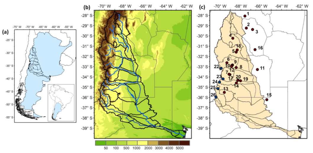
2.1. Study Region
2.2. Observed Data
2.3. Simulated Data
2.4. Singular Spectrum Analysis
2.5. Evaluation and Bias-Correction Methods
3. Results
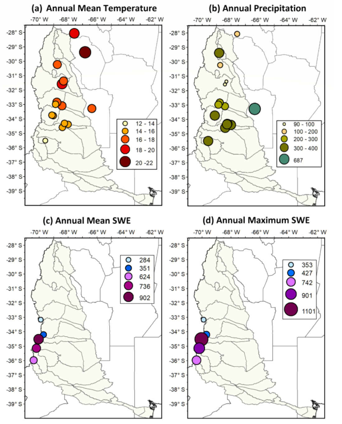
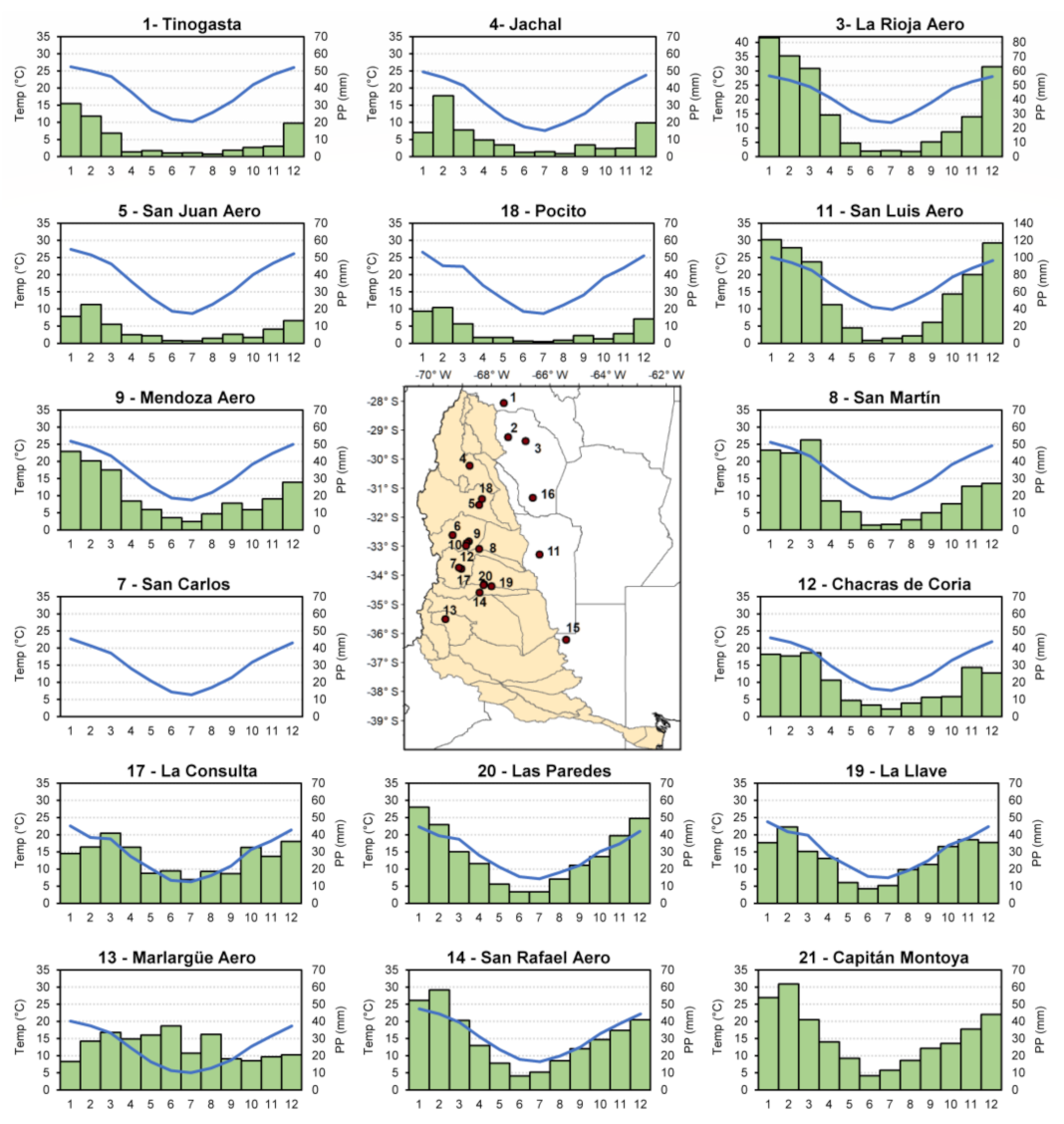
3.1. Climatology
3.2. Variability and Changes
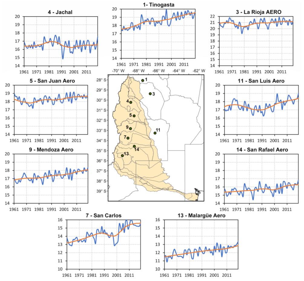
3.2.1. Temperature
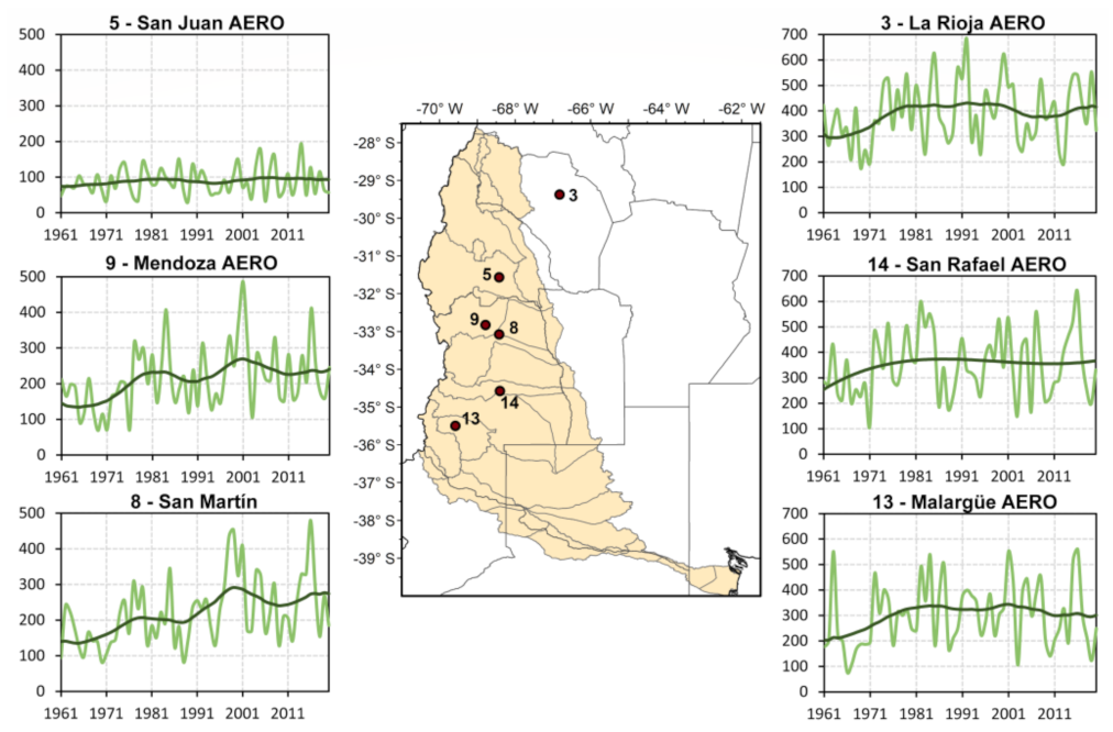
3.2.2. Precipitation
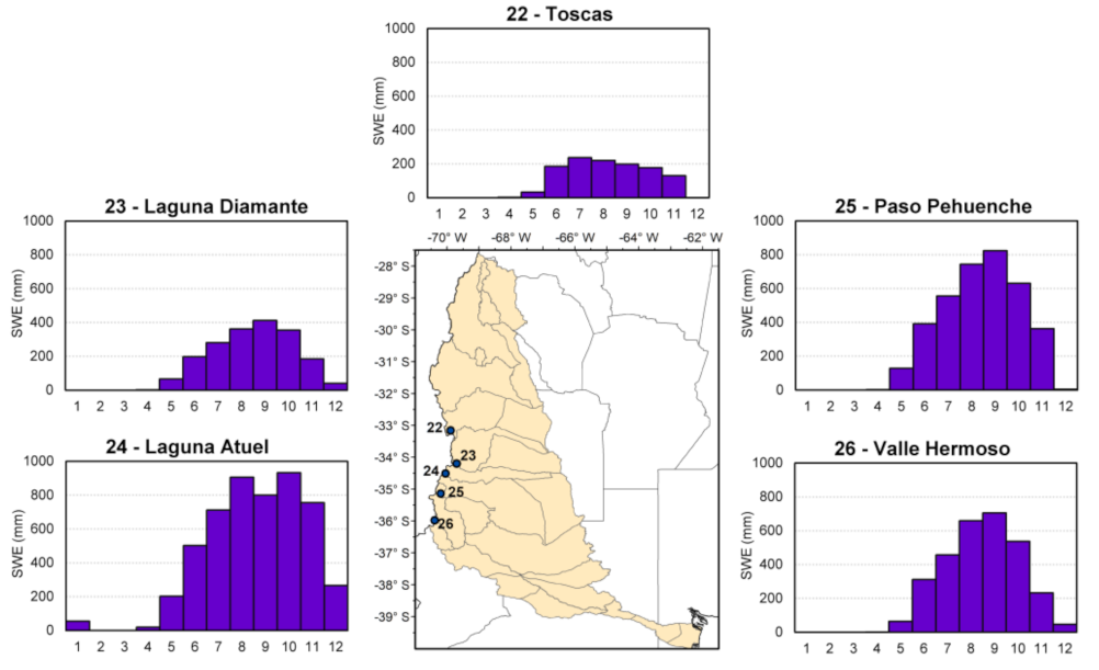
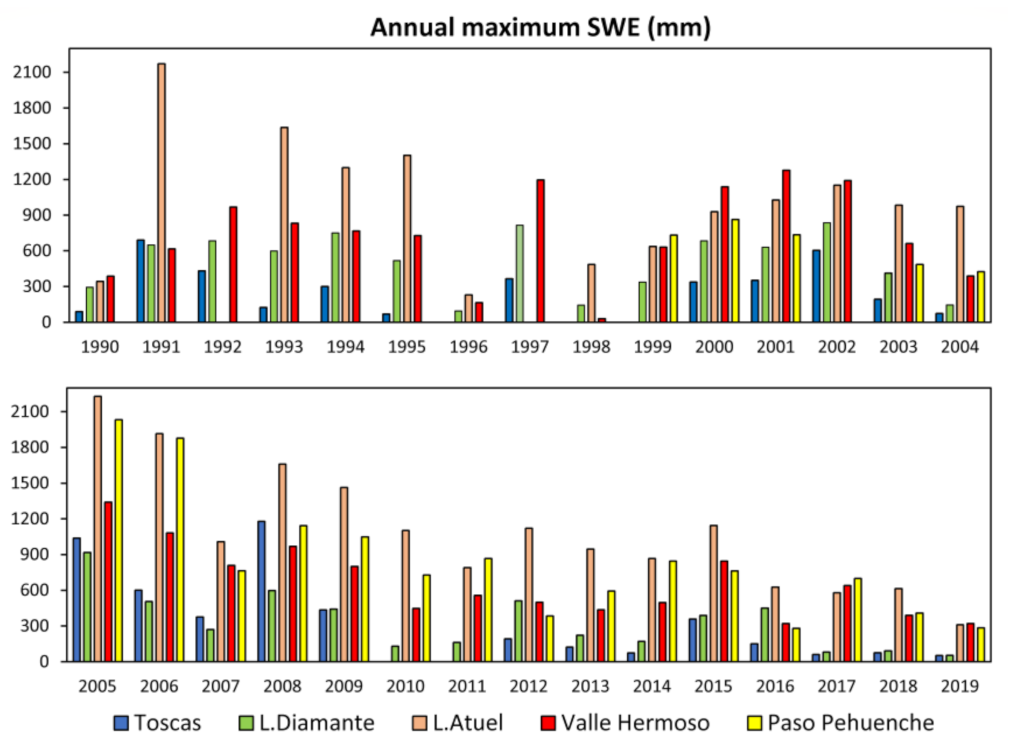
3.2.3. Snow Water Equivalent
3.3. Ability of the Models to Represent the Observed Variables
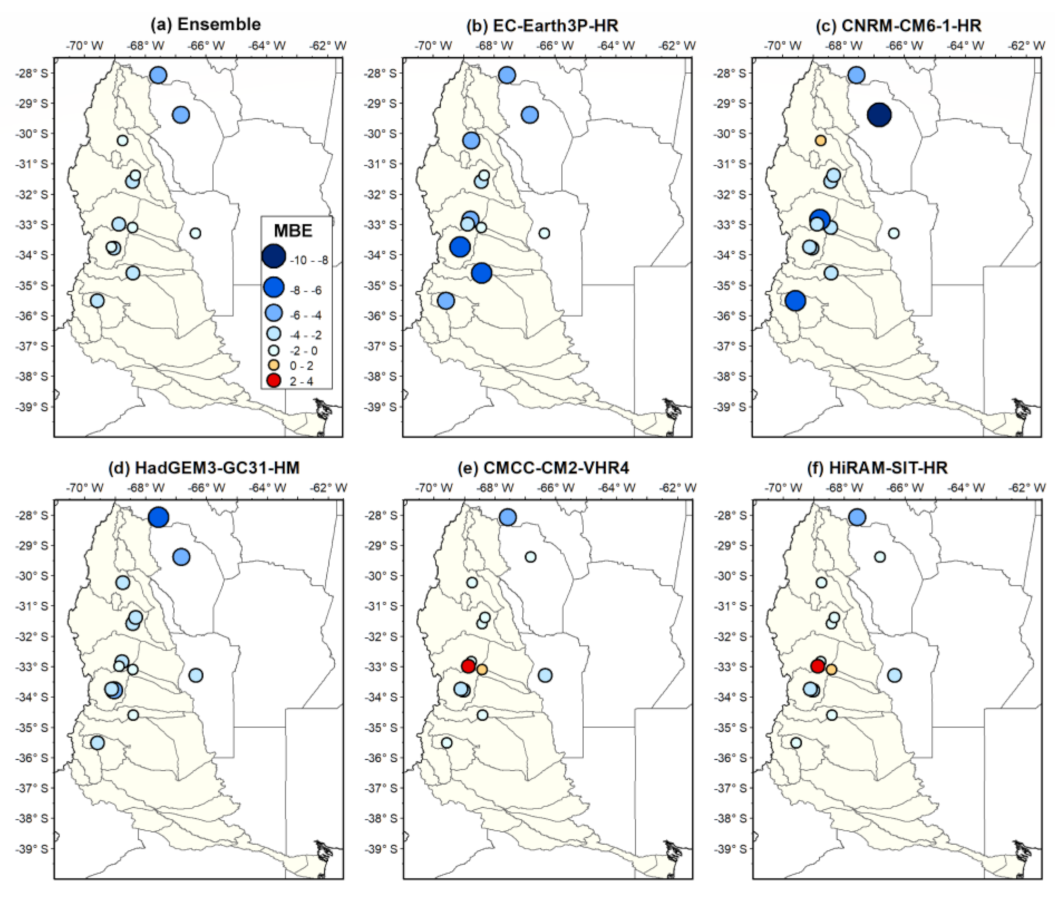
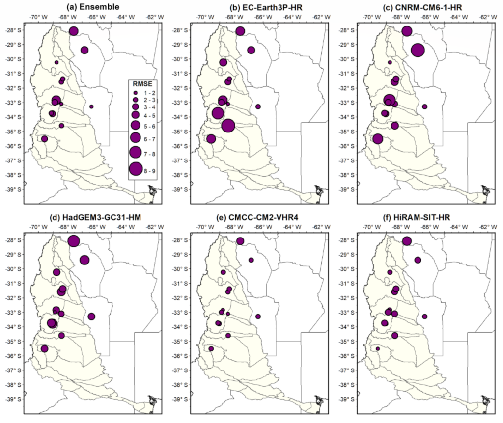
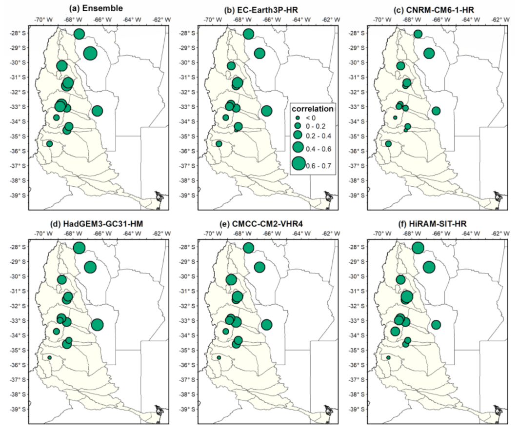
3.3.1. Temperature
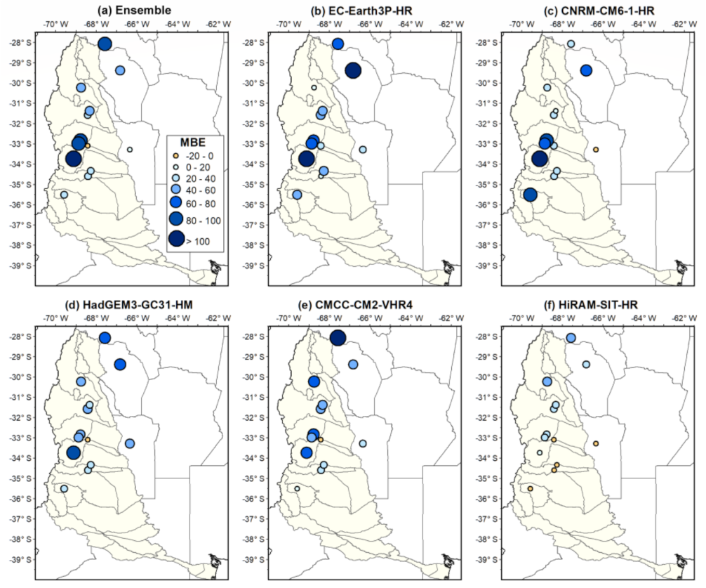
3.3.2. Precipitation
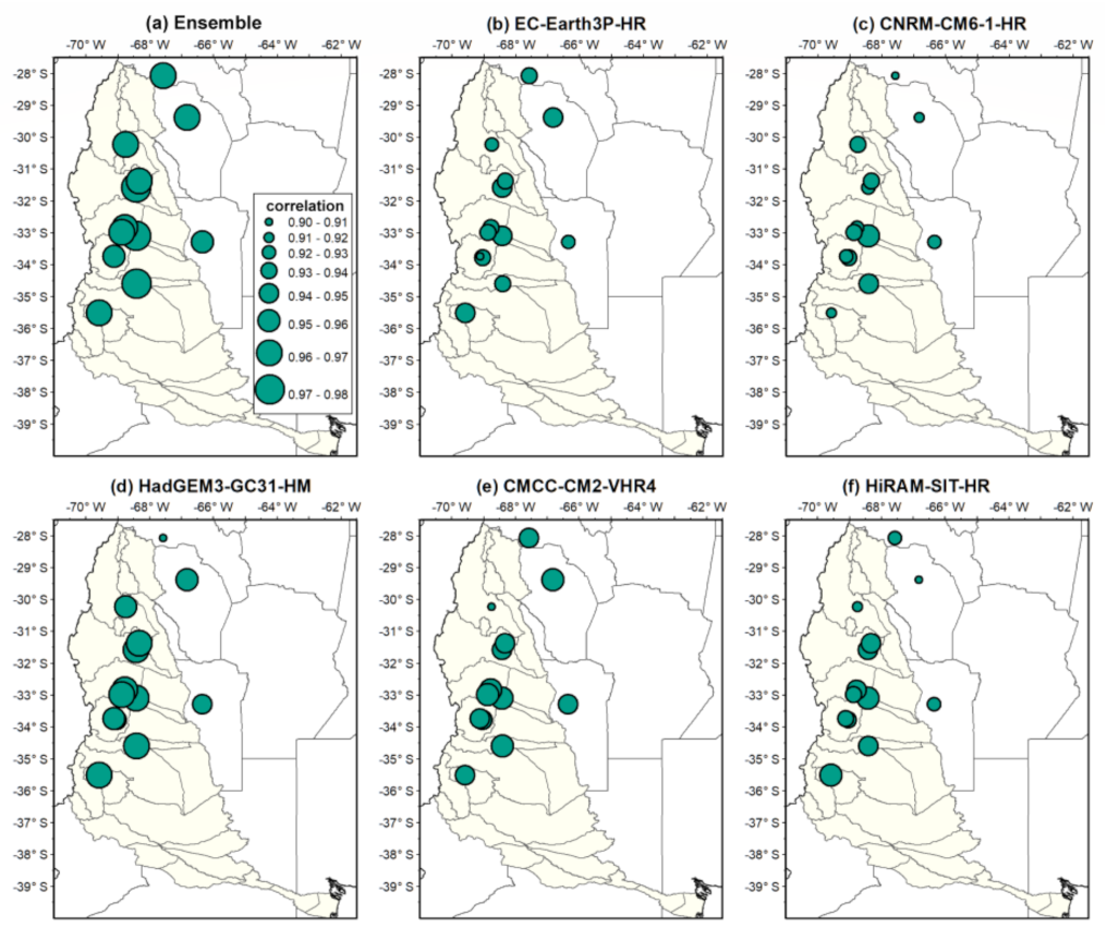
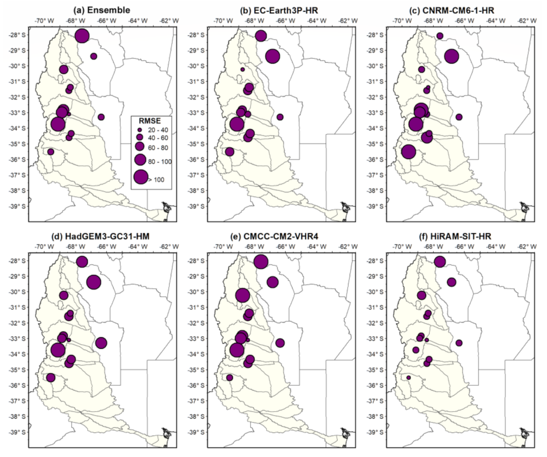
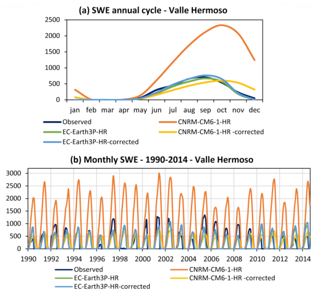
3.3.3. Snow Water Equivalent
3.4. Projected Changes
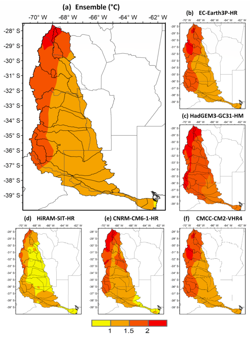
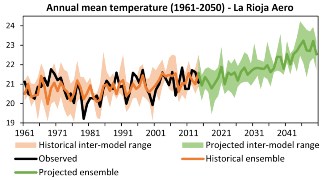
3.4.1. Temperature
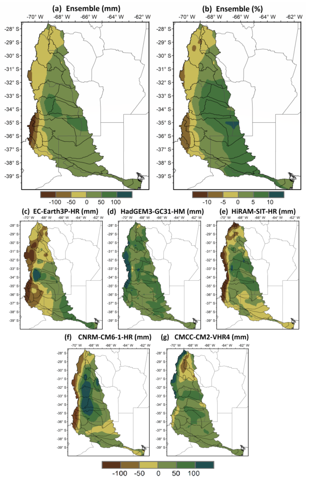
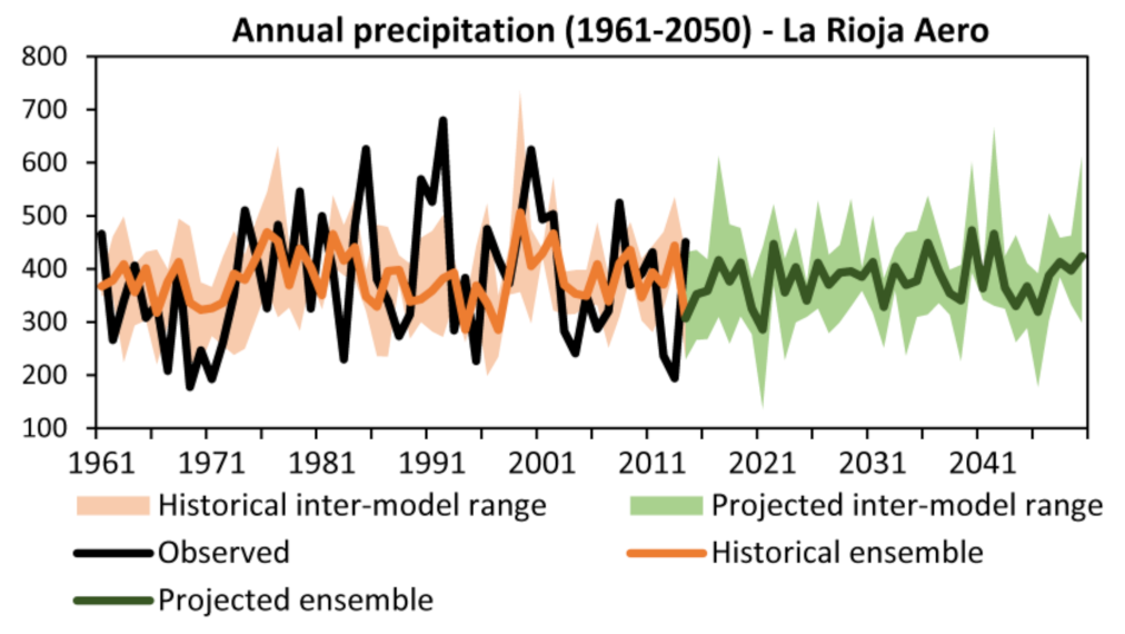
3.4.2. Precipitation
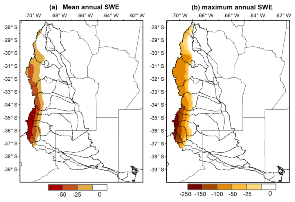
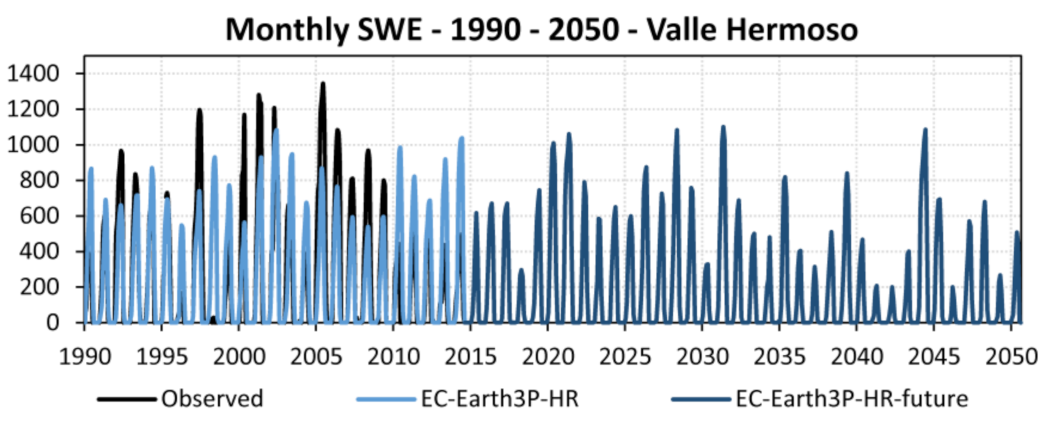
3.4.3. Snow Water Equivalent
4. Discussion and Conclusions
Author Contributions
Funding
Data Availability Statement
Acknowledgments
Conflicts of Interest
Appendix A

| Nº | Station | Components | Trend or Dominant Period (Years/Cycle) | Explained Variance (%) |
|---|---|---|---|---|
| 1 | Tinogasta | T-PC1 | Trend | 55.5 |
| T-PC2/T-PC3 | 8.5 | 14.8 | ||
| T-PC4/T-PC5 | 2.8 | 12.53 | ||
| T-PC3/T-PC4 | 2.6 | 28.2 | ||
| 2 | La Rioja | T-PC1 | Trend | 25.6 |
| T-PC2/T-PC3 | 8.5 | 30 | ||
| T-PC4/T-PC5 | 2.8 | 16.6 | ||
| 3 | Jachal | T-PC1 | Trend | 19.4 |
| T-PC2/T-PC3 | 8.5 | 25.5 | ||
| T-PC4/T-PC5 | 3.74 | 20.4 | ||
| 4 | San Juan Aero | T-PC1 | Trend | 33.7 |
| T-PC2/T-PC3 | 2.85 | 18.2 | ||
| T-PC4/T-PC5 | 4 | 16.14 | ||
| 5 | San Carlos | T-PC1 | Trend | 59 |
| T-PC2/T-PC3 | 8.5 | 19.5 | ||
| T-PC4/T-PC5 | 2.8 | 9.35 | ||
| 6 | Mendoza Aero | T-PC1 | Trend | 37.3 |
| T-PC2/T-PC3 | 8.5 | 20.7 | ||
| T-PC4/T-PC5 | 2.8 | 16.4 | ||
| 7 | San Luis Aero | T-PC1 | Trend | 41.8 |
| T-PC2/T-PC3 | 8.5 | 31.2 | ||
| T-PC4/T-PC5 | 2.3 | 9.3 | ||
| 8 | Malargüe | T-PC1 | Trend | 36.8 |
| T-PC2/T-PC3 | 4 | 20.2 | ||
| T-PC4/T-PC5 | 8.5 | 16.3 | ||
| 9 | San Rafael | T-PC1 | Trend | 24 |
| T-PC2/T-PC3 | 8.5 | 28.7 | ||
| T-PC4/T-PC5 | 4 | 17.8 |
| Nº | Station | Components | Trend or Dominant Period (Years/Cycle) | Explained Variance (%) |
|---|---|---|---|---|
| 1 | La Rioja | T-PC1 y T-PC2 | 8.5 | 35.5 |
| T-PC3 | Trend | 12.6 | ||
| 2 | San Juan Aero | T-PC1 y T-PC2 | 3 | 34 |
| T-PC3 y T-PC4 | 4.2 | 26.4 | ||
| T-PC5 y T-PC6 | 6 | 19.5 | ||
| T-PC9 | Trend | 3.5 | ||
| 3 | San Martin | T-PC1 | Trend | 28.4 |
| T-PC2 y T-PC3 | 7.5 | 32.3 | ||
| T-PC4 y T-PC5 | 2.8 | 17.9 | ||
| 4 | Mendoza Aero | T-PC1 | Trend | 22.6 |
| T-PC3 y T-PC4 | 3.3 | 24.3 | ||
| 5 | Malargüe | T-PC1 y T-PC2 | 10 | 35.8 |
| T-PC3 y T-PC4 | 3.5 | 24.2 | ||
| T-PC8 | Trend | 7.3 | ||
| 6 | San Rafael | T-PC1 y T-PC2 | 8.5 | 36.0 |
| T-PC3 y T-PC4 | 2.6 | 25.8 | ||
| T-PC5 | Trend | 11.2 |
Appendix B


References
- Cai, W.; Cowan, T.; Thatcher, M. Rainfall reductions over Southern hemisphere semi-arid regions: The role of subtropical dry zone expansion. Sci. Rep. 2012, 2, 702. [Google Scholar] [CrossRef]
- Sgroi, L.C.; Lovino, M.; Berbery, E.H.; Müller, G.V. Characteristics of droughts in Argentina’s Core Crop Region. Hydrol. Earth Syst. Sci. 2020, 25, 2475–2490. [Google Scholar] [CrossRef]
- Carril, A.F.; Cavalcanti, I.F.A.; Menéndez, C.G.; Sörensson, A.; López-Franca, N.; Rivera, J.; Robledo, F.; Zaninelli, P.; Ambrizzi, T.; Penalba, O.; et al. Extreme events in the La Plata basin: A retrospective analysis of what we have learned during CLARIS-LPB project. Clim. Res. 2015, 68, 95–116. [Google Scholar] [CrossRef]
- Avila-Diaz, A.; Benezoli, V.; Justino, F.; Torres, R.; Wilson, A. Assessing current and future trends of climate extremes across Brazil based on reanalyses and earth system model projections. Clim. Dyn. 2020, 55, 1403–1426. [Google Scholar] [CrossRef]
- Boisier, J.P.; Rondanelli, R.; Garreaud, R.D.; Muñoz, F. Anthropogenic and natural contributions to the Southeast Pacific precipitation decline and recent megadrought in central Chile. Geophys. Res. Lett. 2016, 43, 413–421. [Google Scholar] [CrossRef]
- Garreaud, R.D.; Alvarez-Garreton, C.; Barichivich, J.; Boisier, J.P.; Christie, D.; Galleguillos, M.; LeQuesne, C.; McPhee, J.; Zambrano-Bigiarini, M. The 2010–2015 megadrought in central Chile: Impacts on regional hydroclimate and vegetation. Hydrol. Earth Syst. Sci. 2017, 21, 6307–6327. [Google Scholar] [CrossRef]
- Skansi, M.; Brunet, M.; Sigró, J.; Aguilar, E.; Arevalo Groening, J.; Bentancur, O.; Castellón Geier, Y.; Correa Amaya, R.; Jácome, H.; Malheiros Ramos, A.; et al. Warming and wetting signals emerging from analysis of changes in climate extreme indices over South America. Glob. Planet. Chang. 2013, 100, 295–307. [Google Scholar] [CrossRef]
- Lovino, M.; Müller, O.; Berbery, E.H.; Müller, G.V. How have daily climate extremes changed in the recent past over northeastern Argentina? Glob. Planet. Chang. 2018, 168, 78–97. [Google Scholar] [CrossRef]
- Cerón, W.L.; Kayano, M.T.; Andreoli, R.V.; Avila-Diaz, A.; Rivera, I.A.; Freitas, E.D.; Martins, J.A.; Souza, R.A.F. Recent intensification of extreme precipitation events in the La Plata Basin in southern South America (1981–2018). Atmos. Res. 2021, 249, 105299. [Google Scholar] [CrossRef]
- Donnelly, C.; Greuell, W.; Andersson, J.; Gerten, D.; Pisacane, G.; Roudier, P.; Ludwig, F. Impacts of climate change on European hydrology at 1.5, 2 and 3 degrees mean global warming above preindustrial level. Clim. Change 2017, 143, 13–26. [Google Scholar] [CrossRef]
- Rivera, J.A.; Otta, S.; Lauro, C.; Zazulie, N. A Decade of Hydrological Drought in Central-Western Argentina. Front. Water 2021, 3, 640544. [Google Scholar] [CrossRef]
- Barros, V.; Boninsegna, J.; Camilloni, I.; Chidiak, M.; Magrín, G.; Rusticucci, M. Climate change in Argentina: Trends, projections, impacts and adaptation. Wiley Interdiscip. Rev. Clim. Chang. 2015, 6, 151–169. [Google Scholar] [CrossRef]
- Rivera, J.A.; Naranjo Tamayo, E.; Viale, M. Water Resources Change in Central-Western Argentina Under the Paris Agreement Warming Targets. Front. Clim. 2020, 2, 587126. [Google Scholar] [CrossRef]
- Masiokas, M.H.; Rabatel, A.; Rivera, A.; Ruiz, L.; Pitte, P.; Ceballos, J.L.; Barcaza, G.; Soruco, A.; Bown, F.; Berthier, E.; et al. A review of the current state and recent changes of the Andean cryosphere. Front. Earth Sci. 2020, 8, 99. [Google Scholar] [CrossRef]
- Rivera, J.A.; Penalba, O.C.; Villalba, R.; Araneo, D.C. Spatio-temporal patterns of the 2010-2015 extreme hydrological drought across the Central Andes, Argentina. Water 2017, 9, 652. [Google Scholar] [CrossRef]
- Zazulie, N.; Rusticucci, M.; Raga, G.B. Regional climate of the Subtropical Central Andes using high-resolution CMIP5 models. Part II: Future projections for the twenty-first century. Clim. Dyn. 2018, 51, 2913–2925. [Google Scholar] [CrossRef]
- Pabón-Caicedo, J.D.; Arias, P.A.; Carril, A.F.; Espinoza, J.C.; Borrel, L.F.; Goubanova, K.; Lavado-Casimiro, W.; Masiokas, M.; Solman, S.; Villalba, R. Observed and Projected Hydroclimate Changes in the Andes. Front. Earth Sci. 2020, 8, 61. [Google Scholar] [CrossRef]
- Spinoni, J.; Barbosa, P.; Bucchignani, E.; Cassano, J.; Cavazos, T.; Christensen, J.H.; Christensen, O.B.; Coppola, E.; Evans, J.; Geyer, B.; et al. Future Global Meteorological Drought Hot Spots: A Study Based on CORDEX Data. J. Clim. 2020, 33, 3635–3661. [Google Scholar] [CrossRef]
- Almazroui, M.; Ashfaq, M.; Islam, M.N.; Kamil, S.; Abid, M.A.; O’Brien, E.; Ismail, M.; Reboita, M.S.; Sörensson, A.A.; Arias, P.A.; et al. Assessment of CMIP6 performance and projected temperature and precipitation changes over South America. Earth Syst. Environ. 2021, 5, 155–183. [Google Scholar] [CrossRef]
- Hock, R.; Bliss, A.; Marzeion, B.; Giesen, R.H.; Hirabayashi, Y.; HUSS, M.; Radic, V.; Slangen, A.B.A. GlacierMIP–A model intercomparison of global-scale glacier mass-balance models and projections. J. Glaciol. 2019, 65, 453–467. [Google Scholar] [CrossRef]
- Arias, P.A.; Garreaud, R.; Poveda, G.; Espinoza, J.C.; Molina-Carpio, J.; Masiokas, M.; Viale, M.; Scaff, L.; van Oevelen, P.J. Hydroclimate of the Andes part II: Hydroclimate variability and sub-continental patterns. Front. Earth Sci. 2021, 8, 505467. [Google Scholar] [CrossRef]
- Rivera, J.A.; Arnould, G. Evaluation of the ability of CMIP6 models to simulate precipitation over Southwestern South America: Climatic features and long-term trends (1901–2014). Atmos. Res. 2020, 241, 104953. [Google Scholar] [CrossRef]
- Mindlin, J.; Shepherd, T.G.; Vera, C.S.; Osman, M.; Zappa, G.; Lee, R.W.; Hodges, K.I. Storyline description of Southern hemisphere midlatitude circulation and precipitation response to greenhouse gas forcing. Clim. Dyn. 2020, 54, 4399–4421. [Google Scholar] [CrossRef]
- Villamayor, J.; Khodri, M.; Villalba, R.; Valérie Daux. Causes of the long-term variability of southwestern South America precipitation in the IPSL-CM6A-LR model. Clim. Dyn. 2021, 57, 2391–2414. [Google Scholar] [CrossRef]
- Rivera, J.A.; Araneo, D.C.; Penalba, O.C. Threshold level approach for streamflow droughts analysis in the Central Andes of Argentina: A climatological assessment. Hydrol. Sci. J. 2017, 62, 1949–1964. [Google Scholar] [CrossRef]
- Berri, G.J.; Bianchi, E.; Müller, G.V. El Niño and La Niña influence on mean river flows of southern South America along the twentieth century. Hydrol. Sci. J. 2019, 64, 900–909. [Google Scholar] [CrossRef]
- Lauro, C.; Vich, A.I.; Moreiras, S.M. Streamflow variability and its relationship with climate indices in western rivers of Argentina. Hydrol. Sci. J. 2019, 64, 607–619. [Google Scholar] [CrossRef]
- Bereciartua, P.; Antunez, N.; Manzelli, L.; López, P.; Callau Poduje, A.C. Estudio Integral de la Cuenca del Río Desaguadero-Salado-Chadileuvú-Curacó. Subsecretaría de Recursos Hídricos de la Nación—Universidad de Buenos Aires 2009. Available online: https://cuencadesaguadero.weebly.com/biblioteca.html (accessed on 2 March 2023).
- Viale, M.; Nuñez, M.N. Climatology of winter orographic precipitation over the subtropical central Andes and associated synoptic and regional characteristics. J. Hydrometeorol. 2011, 12, 481–507. [Google Scholar] [CrossRef]
- Doyle, M.E. Observed and simulated changes in precipitation seasonality in Argentina. Int. J. Climatol. 2020, 40, 1716–1737. [Google Scholar] [CrossRef]
- Viale, M.; Bianchi, E.; Cara, L.; Ruiz, L.E.; Villalba, R.; Pitte, P.; Masiokas, M.; Rivera, J.; Zalazar, L. Contrasting climates at both sides of the Andes in Argentina and Chile. Front. Earth Sci. 2019, 7, 69. [Google Scholar] [CrossRef]
- World Meteorological Organization (WMO). WMO Guidelines on the Calculation of Climate Normals. WMO-No. 1203; WMO: Geneva, Switzerland; p. 29. Available online: https://library.wmo.int/doc_num.php?explnum_id=4166 (accessed on 21 April 2023).
- Masiokas, M.; Villalba, R.; Luckman, B.; Le Quesne, C.; Aravena, J.C. Snowpack variations in the Central Andes of Argentina and Chile, 1951–2005: Large-scale atmospheric influences and implications for water resources in the region. J. Clim. 2006, 19, 6334–6352. [Google Scholar] [CrossRef]
- Haarsma, R.J.; Roberts, M.J.; Vidale, P.L.; Senior, C.A.; Bellucci, A.; Bao, Q.; Bao, Q.; Chang, P.; Corti, S.; Fučkar, N.S.; et al. High Resolution Model Intercomparison Project (HighResMIP v1.0) for CMIP6. Geosci. Model Dev. 2016, 9, 4185–4208. [Google Scholar] [CrossRef]
- Eyring, V.; Bony, S.; Meehl, G.A.; Senior, C.A.; Stevens, B.; Stouffer, R.J.; Taylor, K.E. Overview of the coupled model intercomparison project phase 6 (CMIP6) experimental design and organization. Geosci. Model. Dev. 2016, 9, 1937–1958. [Google Scholar] [CrossRef]
- Zazulie, N.; Rusticucci, M.; Raga, G.B. Regional climate of the subtropical Central Andes using high resolution CMIP5 models. Part I: Past performance (1980–2005). Clim. Dyn. 2017, 49, 3937–3957. [Google Scholar] [CrossRef]
- Ghil, M.; Allen, M.; Dettinger, M.; Ide, K.; Kondrashov, D.; Mann, M.; Robertson, A.; Saunders, A.; Tian, Y.; Varadi, F.; et al. Advanced spectral methods for climatic time series. Rev. Geophys. 2002, 40, 3-1–3-41. [Google Scholar] [CrossRef]
- Wilks, D.S. Statistical Methods in the Atmospheric Sciences, 2nd ed.; Academic Press: Cambridge, MA, USA, 2006; p. 627. [Google Scholar]
- Ghil, M.; Vautard, R. Interdecadal oscillations and the warming trend in global temperature time series. Nature 1991, 350, 324–327. [Google Scholar] [CrossRef]
- Vautard, R. Patterns in Time: SSA and MSSA. In Analysis of Climate Variability; Von Storch, H., Navarra, A., Eds.; Springer: Berlin/Heidelberg, Germany, 1999; pp. 265–286. [Google Scholar] [CrossRef]
- Allen, M.R.; Smith, L.A. Monte Carlo SSA: Detecting irregular oscillations in the presence of colored noise. J. Clim. 1996, 9, 3373–3404. [Google Scholar] [CrossRef]
- Déqué, M. Continuous variables. In Forecast Verification—a Practitioner’s Guide in Atmospheric Science, 2nd ed.; Jolliffe, I.T., Stephenson, D.V., Eds.; John Wiley and Sons: Hoboken, NJ, USA, 2012; pp. 97–120. [Google Scholar]
- Maraun, D.; Wetterhall, F.; Ireson, A.; Chandler, R.; Kendon, E.; Widmann, M.; Brienen, S.; Rust, H.; Sauter, T.; Themel, M.; et al. Precipitation downscaling under climate change: Recent developments to bridge the gap between dynamical models and the end user. Rev. Geophys. 2010, 48, RG3003. [Google Scholar] [CrossRef]
- IPCC. Climate Change 2021: The Physical Science Basis. Contribution of Working Group I to the Sixth Assessment Report of the Intergovernmental Panel on Climate Change; Masson-Delmotte, V.P., Zhai, A., Pirani, S.L., Connors, C., Péan, S., Berger, N., Caud, Y., Chen, L., Goldfarb, M.I., Gomis, M., Eds.; Cambridge University Press: Cambridge, UK; New York, NY, USA, 2021; in press. [Google Scholar]
- Lehner, F.; Deser, C.; Maher, N.; Marotzke, J.; Fischer, E.M.; Brunner, L.; Knutti, R.; Hawkins, E. Partitioning climate projection uncertainty with multiple large ensembles and CMIP5/6. Earth Syst. Dynam. 2020, 11, 491–508. [Google Scholar] [CrossRef]
- Camisay, M.F.; Rivera, J.A.; Matteo, L.; Morichetti, P.; Mackern, M.V. Estimation of integrated water vapor from GNSS ground stations over Central-Western Argentina. Role in the development of regional precipitation events. J. Atmosph. Sol. Terrest. Phys. 2020, 197, 105143. [Google Scholar] [CrossRef]
- Garbarini, E.M.; González, M.H.; Rolla, A.L. The influence of Atlantic High on seasonal rainfall in Argentina. Int. J. Climatol. 2019, 39, 4688–4702. [Google Scholar] [CrossRef]
- Hurtado, S.I.; Agosta, E.A. El Niño Southern Oscillation-related precipitation anomaly variability over eastern subtropical South America: Atypical precipitation seasons. Int. J. Climatol. 2021, 41, 3793–3812. [Google Scholar] [CrossRef]
- Cabré, F.; Nuñez, M. Impacts of climate change on viticulture in Argentina. Reg. Environ. Chang. 2020, 20, 12. [Google Scholar] [CrossRef]


| # | Station | Lat | Lon | masl | Missing Values 1961–2020 (%) | Missing Values 1995–2014 (%) | |||
|---|---|---|---|---|---|---|---|---|---|
| Tmean | PP | Tmean | PP | Snow | |||||
| 1 | Tinogasta | −28.07 | −67.57 | 1201 | 4.3 | 10.3 | 0.0 | 0.0 | |
| 2 | Chilecito Aero | −29.24 | −67.43 | 945 | 64.4 | 40.8 | 84.6 | 0.0 | |
| 3 | La Rioja Aero | −29.38 | −66.82 | 429 | 3.8 | 0.6 | 0.0 | 0.0 | |
| 4 | Jáchal | −30.23 | −68.75 | 1175 | 4.7 | 11.9 | 0.0 | 0.0 | |
| 5 | San Juan Aero | −31.58 | −68.42 | 598 | 3.5 | 3.6 | 0.0 | 0.0 | |
| 6 | Uspallata | −32.62 | −69.33 | 1891 | 27.9 | 57.1 | 12.9 | 29.2 | |
| 7 | San Carlos | −33.78 | −69.03 | 940 | 8.8 | 54.2 | 0.0 | --- | |
| 8 | San Martín | −33.09 | −68.42 | 653 | 1.4 | 1.0 | 0.0 | 0.0 | |
| 9 | Mendoza Aero | −32.84 | −68.78 | 704 | 3.5 | 0.0 | 0.0 | 0.0 | |
| 10 | Mendoza Obs | −32.89 | −68.85 | 827 | 5.3 | 0.3 | 0.0 | 0.0 | |
| 11 | San Luis Aero | −33.28 | −66.35 | 713 | 1.9 | 0.8 | 0.0 | 0.0 | |
| 12 | Chacras de Coria | −32.99 | −68.87 | 921 | 6.0 | 14.3 | 0.0 | 8.0 | |
| 13 | Malargüe Aero | −35.51 | −69.58 | 1425 | 4.4 | 0.4 | 0.0 | 0.0 | |
| 14 | San Rafael Aero | −34.59 | −68.40 | 748 | 0.6 | 0.1 | 0.0 | 0.0 | |
| 15 | Victorica | −36.22 | −65.43 | 312 | 30.8 | 35.4 | 16.7 | 21.3 | |
| 16 | Chepes | −31.34 | −66.58 | 658 | 29.7 | 19.3 | 42.9 | 25.8 | |
| 17 | La Consulta | −33.74 | −69.12 | 940 | 0.4 | 0.0 | |||
| 18 | Pocito | −31.37 | −68.32 | 618 | 0.4 | 0.0 | |||
| 19 | La Llave | −34.38 | −68.00 | 555 | 25.8 | 16.7 | |||
| 20 | Las Paredes | −34.31 | −68.25 | 813 | 21.3 | 17.1 | |||
| 21 | Capitán Montoya | −34.34 | −68.27 | 791 | --- | 0.0 | |||
| Stations with snow data | |||||||||
| 22 | Toscas | −33.16 | −69.89 | 3000 | 31.4 | ||||
| 23 | Laguna Diamante | −34.2 | −69.70 | 3301 | 10.7 | ||||
| 24 | Laguna Atuel | −34.51 | −70.05 | 3423 | 12.9 | ||||
| 25 | Paso Pehuenche | −35.14 | −70.20 | 2253 | 33.6 | ||||
| 26 | Valle Hermoso | −35.98 | −70.39 | 2555 | 11.4 | ||||
| Model | Institution, Country | Atmospheric Resolution (°lon × °lat) | |
|---|---|---|---|
| 1 | EC-Earth3P-HR * | EC-Earth Consortium | 0.35 × 0.35 |
| 2 | CNRM-CM6-1-HR * | CNRM-CERFACS, France | 0.5 × 0.5 |
| 3 | HadGEM3-GC31-HM | MOHC, UK | 0.35 × 0.235 |
| 4 | CMCC-CM2-VHR4 | CMCC, Italy | 0.31 × 0.23 |
| 5 | HiRAM-SIT-HR | AS-RCEC, Taiwan | 0.23 × 0.23 |
| CNRM-CM6-1-HR | |||||
|---|---|---|---|---|---|
| # | Station | MBE | MBE% | RMSE | r |
| 1 | Toscas | 8008.5 | 8207.2 | 9557.3 | 0.049 |
| 2 | Laguna Diamante | 358.5 | 199.1 | 523.9 | 0.493 |
| 3 | Laguna Atuel | 7168.7 | 1581.4 | 7667.3 | 0.290 |
| 4 | Paso Pehuenche | 2850.9 | 936.1 | 3880.3 | 0.241 |
| 5 | Valle Hermoso | 734.0 | 287.1 | 1075.1 | 0.585 |
| EC-Earth3P-HR | |||||
| # | Station | MBE | MBE% | RMSE | r |
| 1 | Toscas | 156.2 | 160.1 | 360.9 | 0.120 |
| 2 | Laguna Diamante | −4.5 | −2.5 | 223.9 | 0.537 |
| 3 | Laguna Atuel | −54.5 | −12.0 | 508.9 | 0.477 |
| 4 | Paso Pehuenche | −8.4 | −2.8 | 288.1 | 0.578 |
| 5 | Valle Hermoso | −32.5 | −12.7 | 254.0 | 0.710 |
Disclaimer/Publisher’s Note: The statements, opinions and data contained in all publications are solely those of the individual author(s) and contributor(s) and not of MDPI and/or the editor(s). MDPI and/or the editor(s) disclaim responsibility for any injury to people or property resulting from any ideas, methods, instructions or products referred to in the content. |
© 2023 by the authors. Licensee MDPI, Basel, Switzerland. This article is an open access article distributed under the terms and conditions of the Creative Commons Attribution (CC BY) license (https://creativecommons.org/licenses/by/4.0/).
Share and Cite
Müller, G.V.; Lovino, M.A. Variability and Changes in Temperature, Precipitation and Snow in the Desaguadero-Salado-Chadileuvú-Curacó Basin, Argentina. Climate 2023, 11, 135. https://doi.org/10.3390/cli11070135
Müller GV, Lovino MA. Variability and Changes in Temperature, Precipitation and Snow in the Desaguadero-Salado-Chadileuvú-Curacó Basin, Argentina. Climate. 2023; 11(7):135. https://doi.org/10.3390/cli11070135
Chicago/Turabian StyleMüller, Gabriela V., and Miguel A. Lovino. 2023. "Variability and Changes in Temperature, Precipitation and Snow in the Desaguadero-Salado-Chadileuvú-Curacó Basin, Argentina" Climate 11, no. 7: 135. https://doi.org/10.3390/cli11070135
APA StyleMüller, G. V., & Lovino, M. A. (2023). Variability and Changes in Temperature, Precipitation and Snow in the Desaguadero-Salado-Chadileuvú-Curacó Basin, Argentina. Climate, 11(7), 135. https://doi.org/10.3390/cli11070135