


Wind–Wave Conditions and Change in Coastal Landforms at the Beach–Dune Barrier of Cesine Lagoon (South Italy)


Abstract
1. Introduction
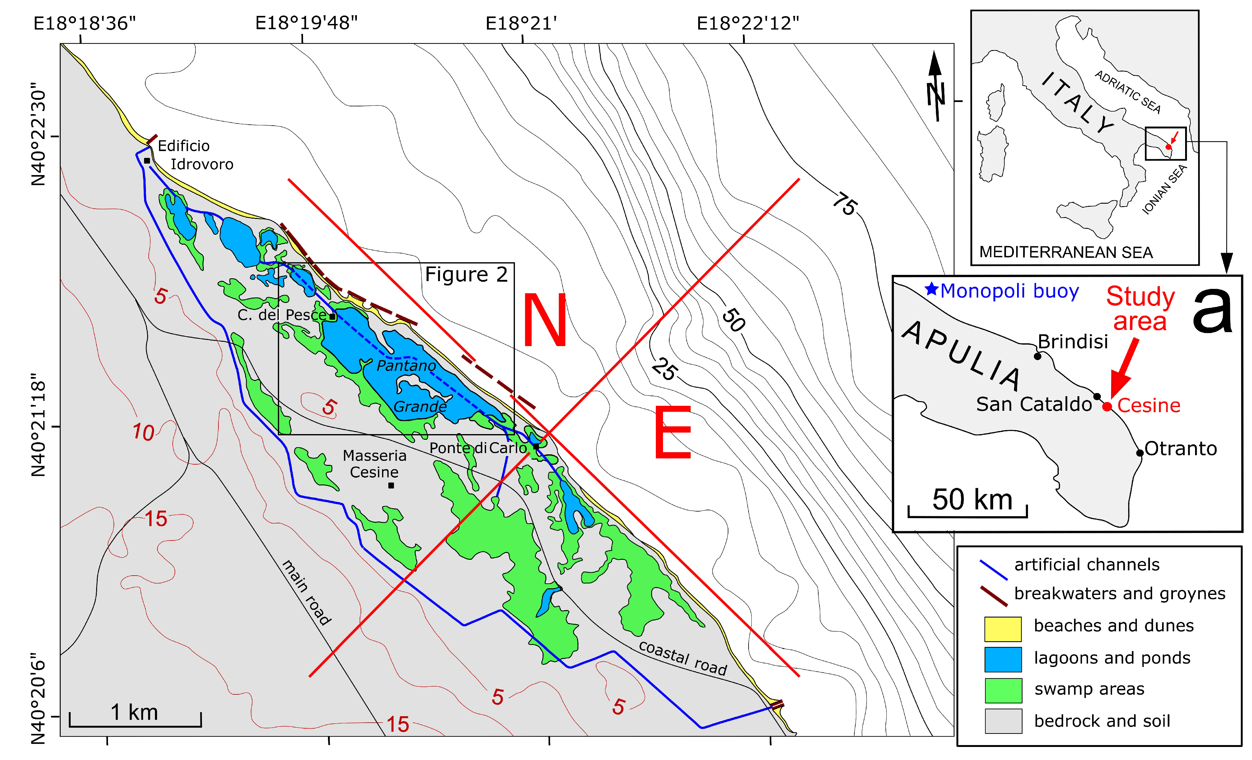
2. Study Area
2.1. Geological–Environmental Setting
2.2. Wind and Wave Climates
3. Materials and Methods
3.1. Meteorological Investigation
3.2. Geomorphological Investigation
4. Results
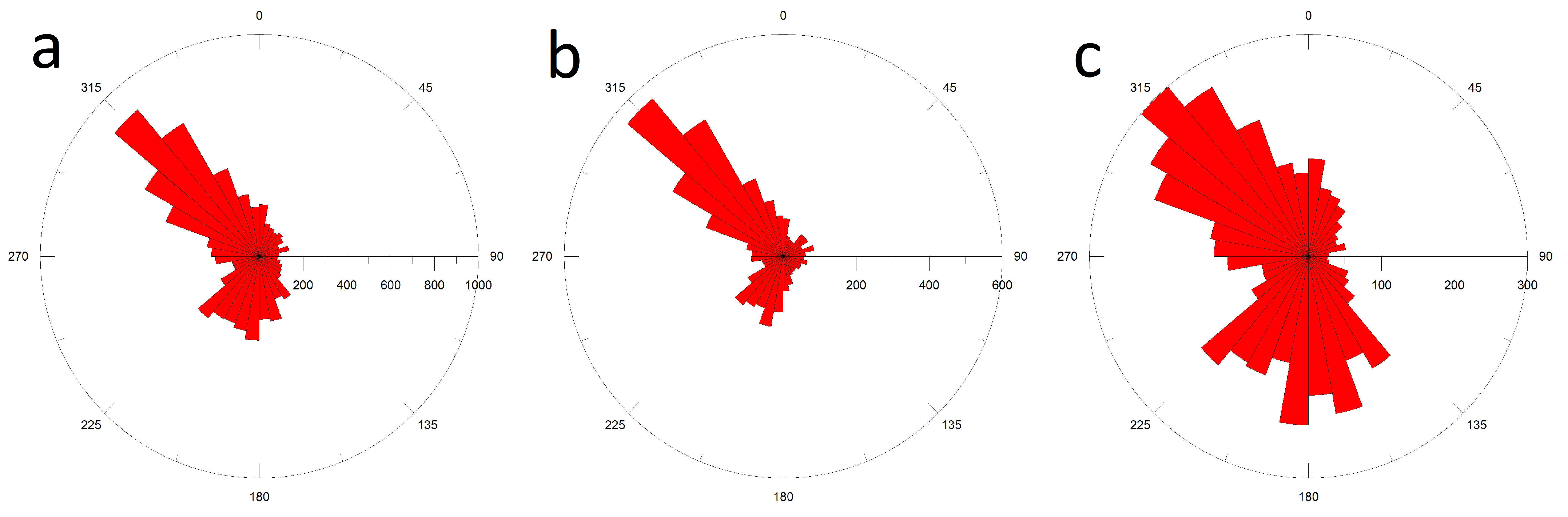
4.1. Wind–Wave Conditions
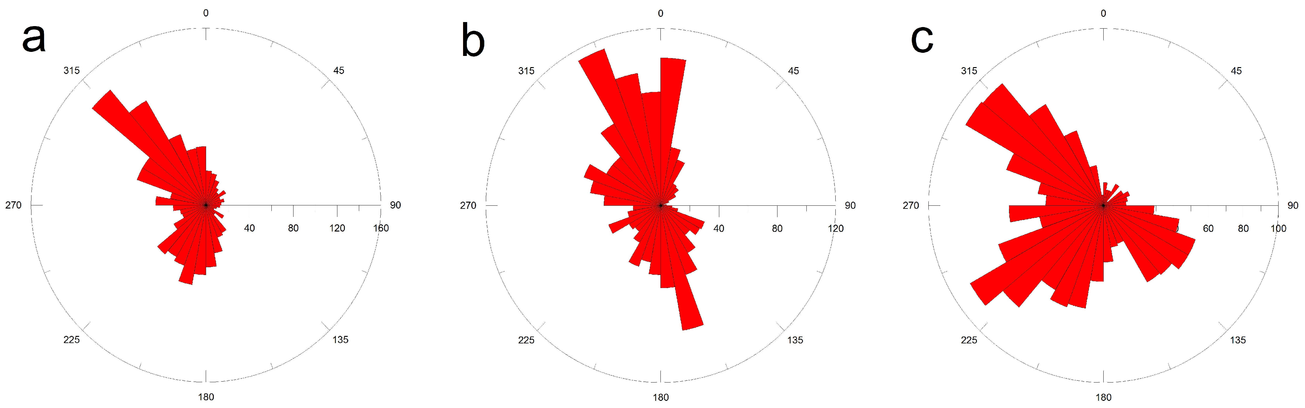
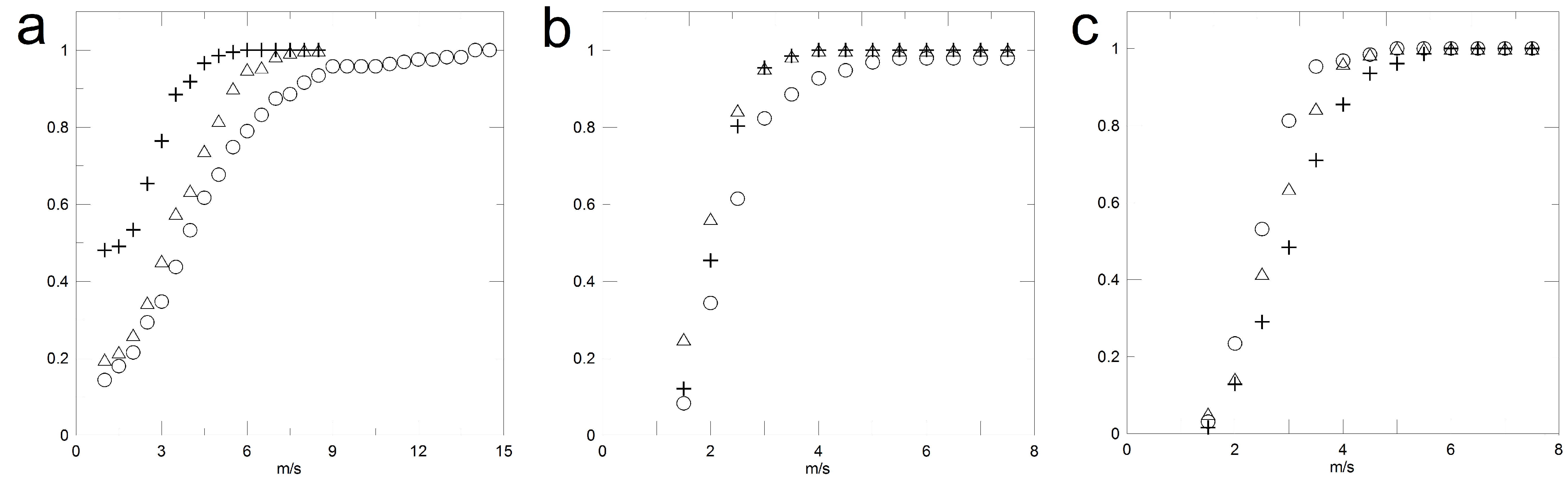
4.1.1. Wind Statistics
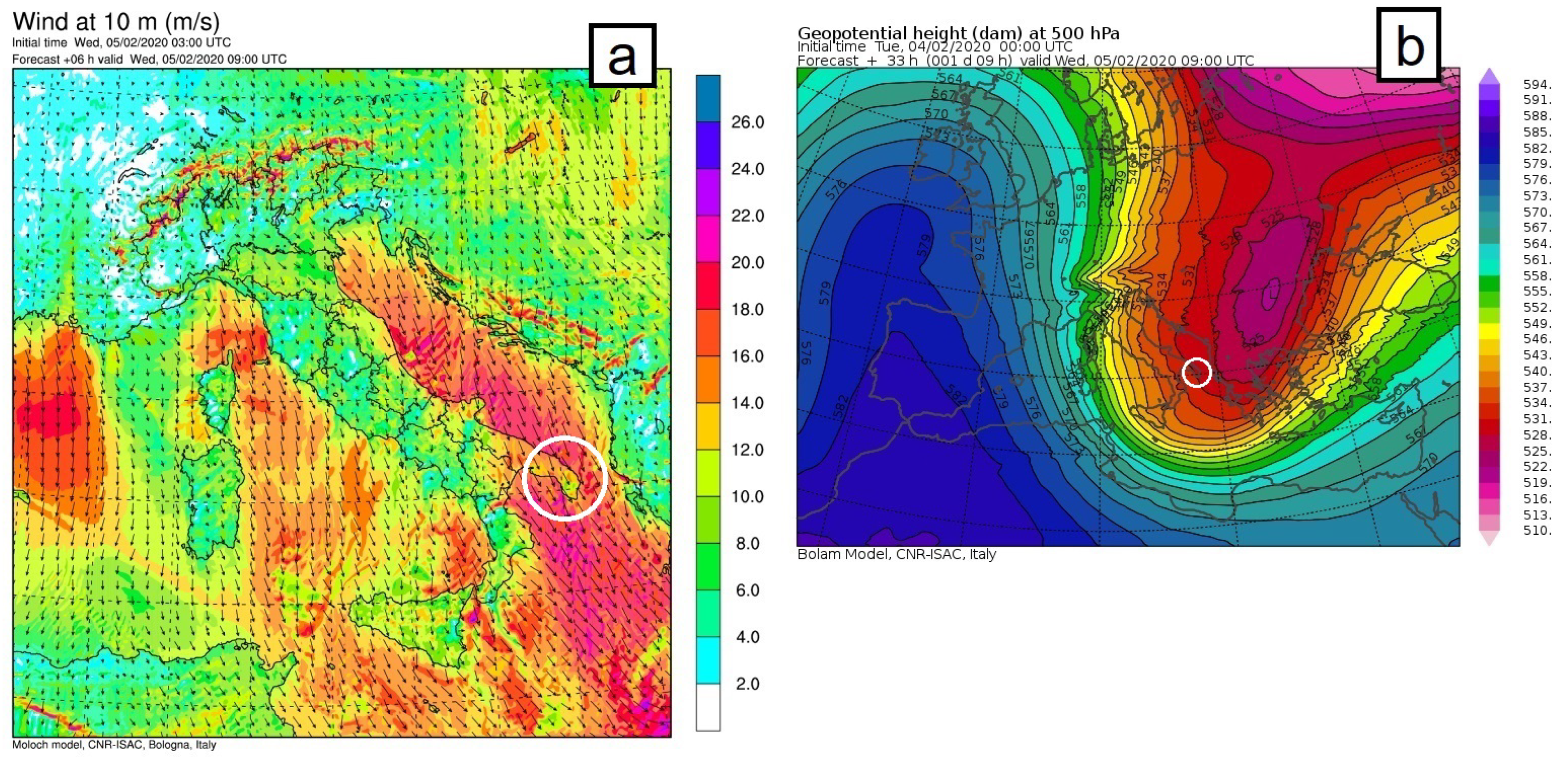
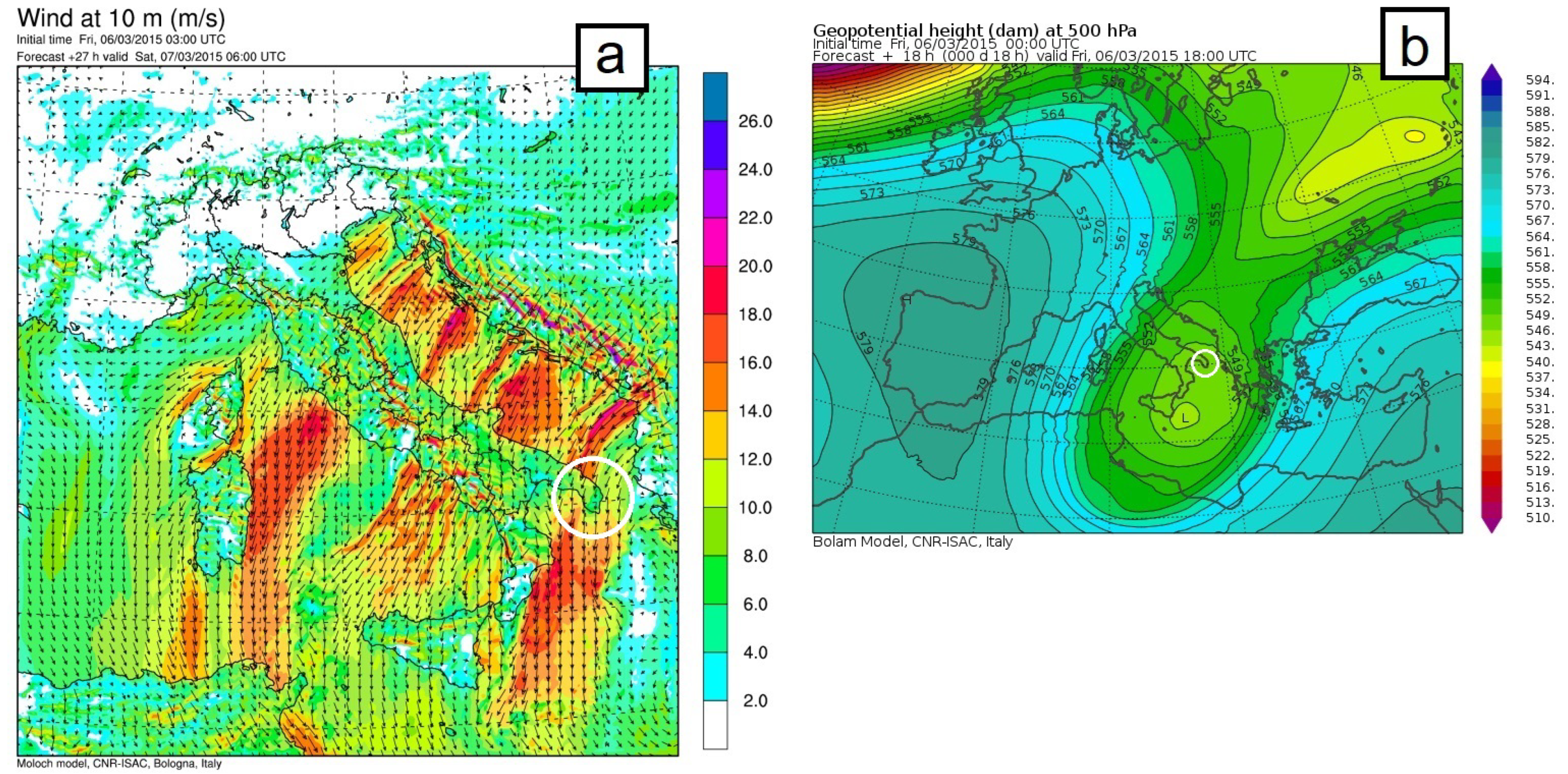
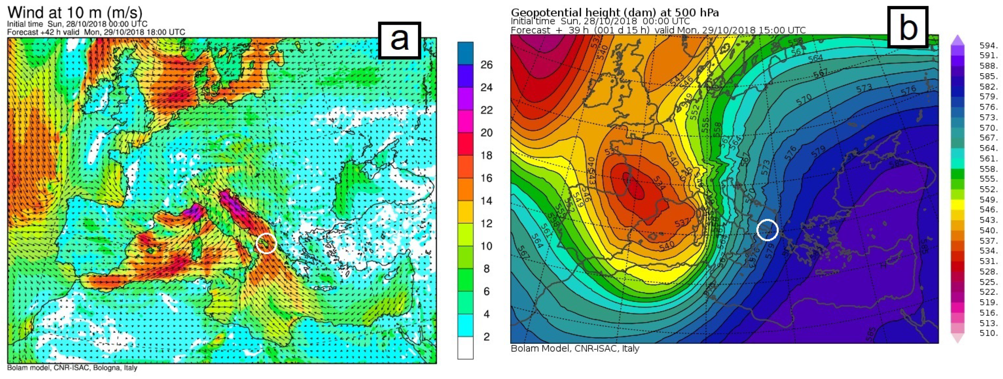
4.1.2. Coastal Storms
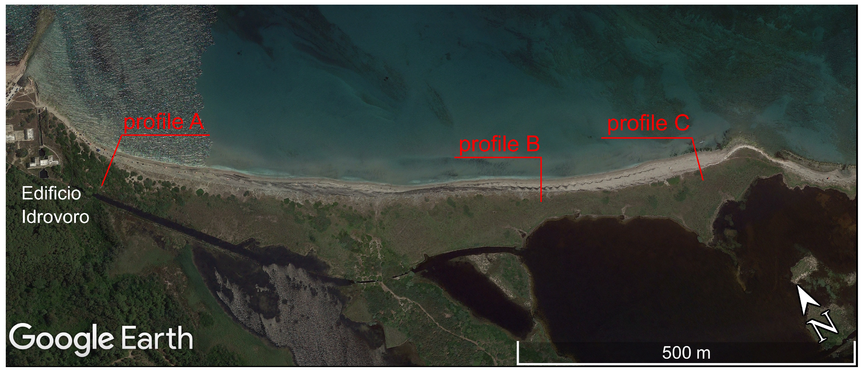
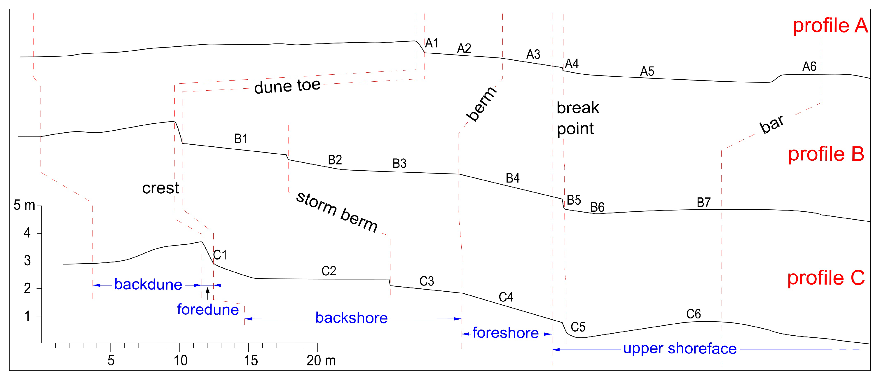
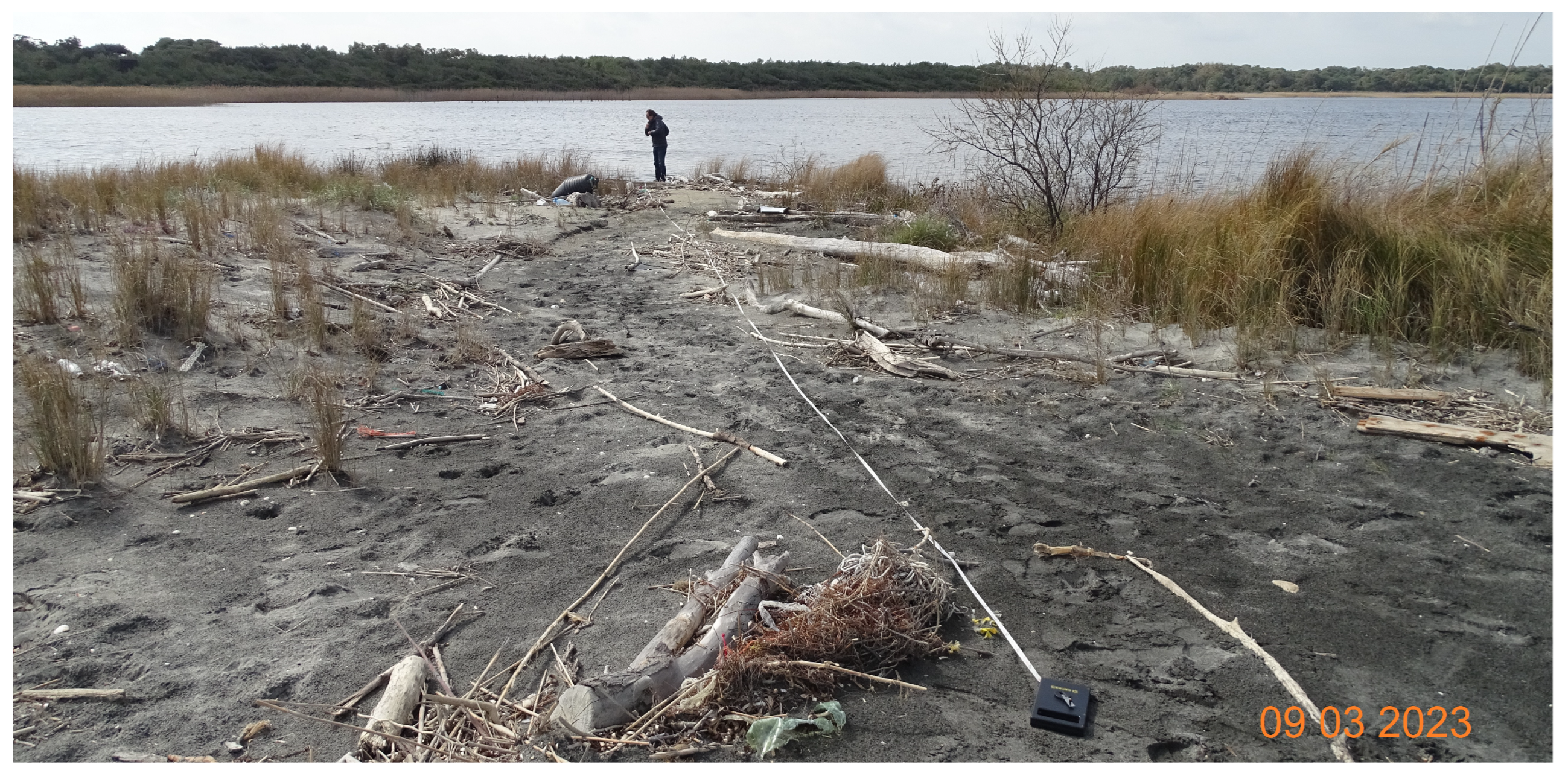
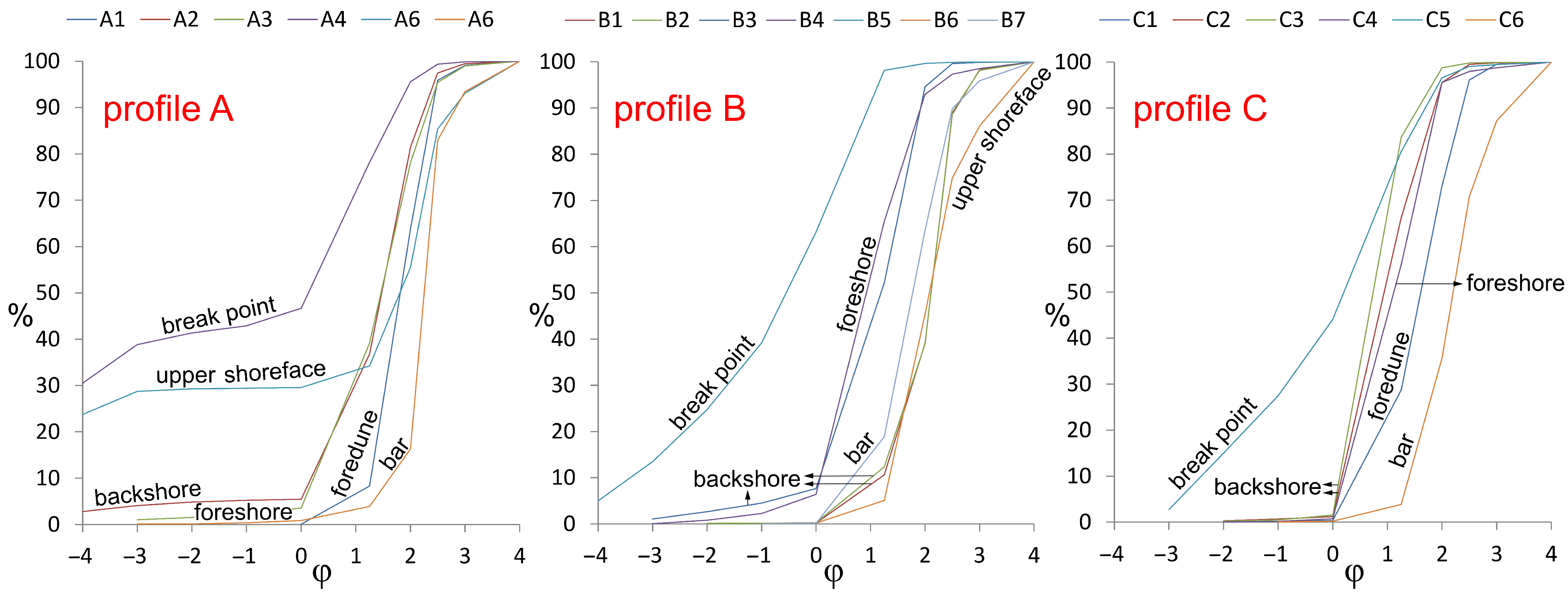
4.2. Barrier Profiling and Sediment Grain Size Check
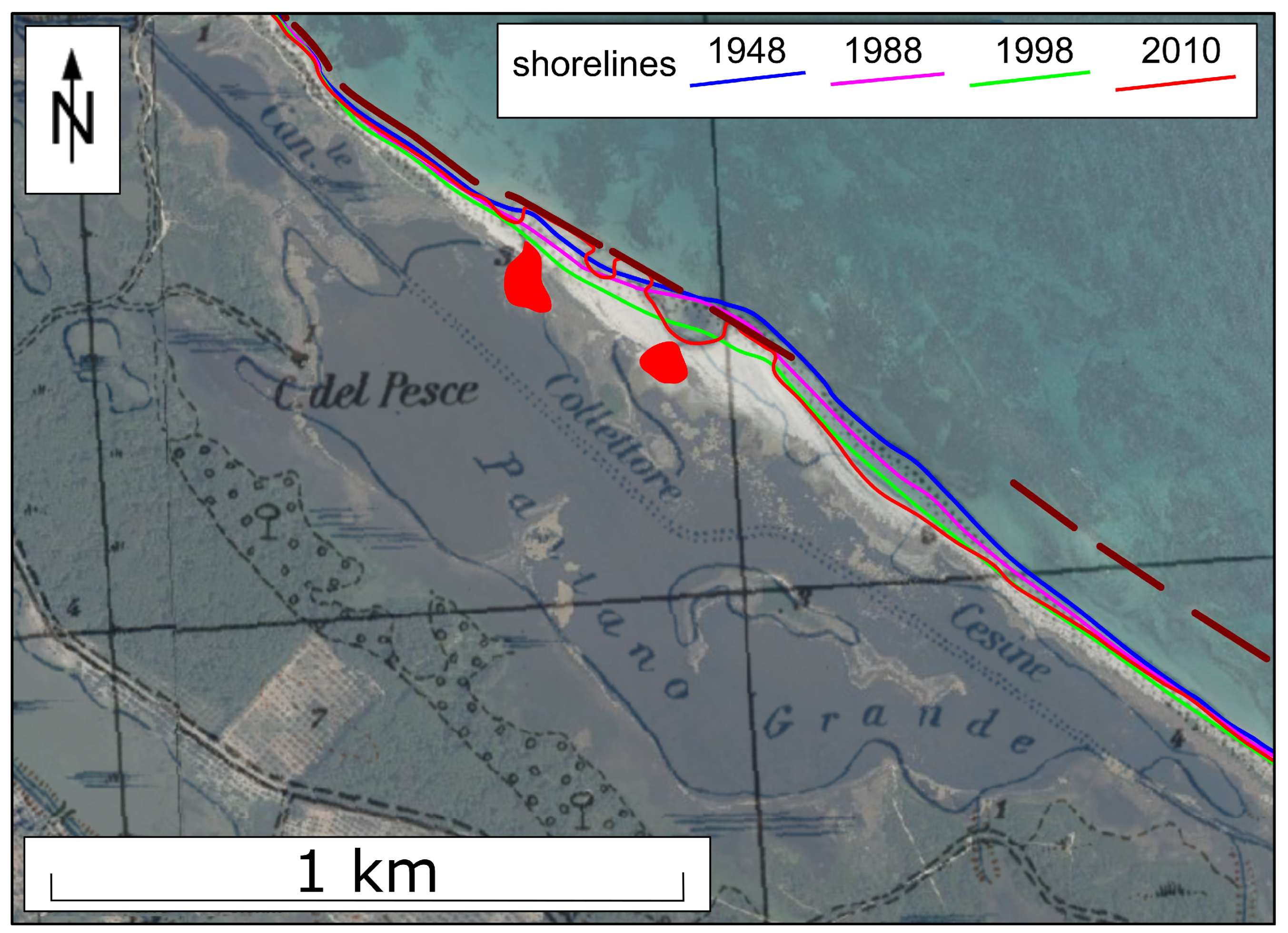
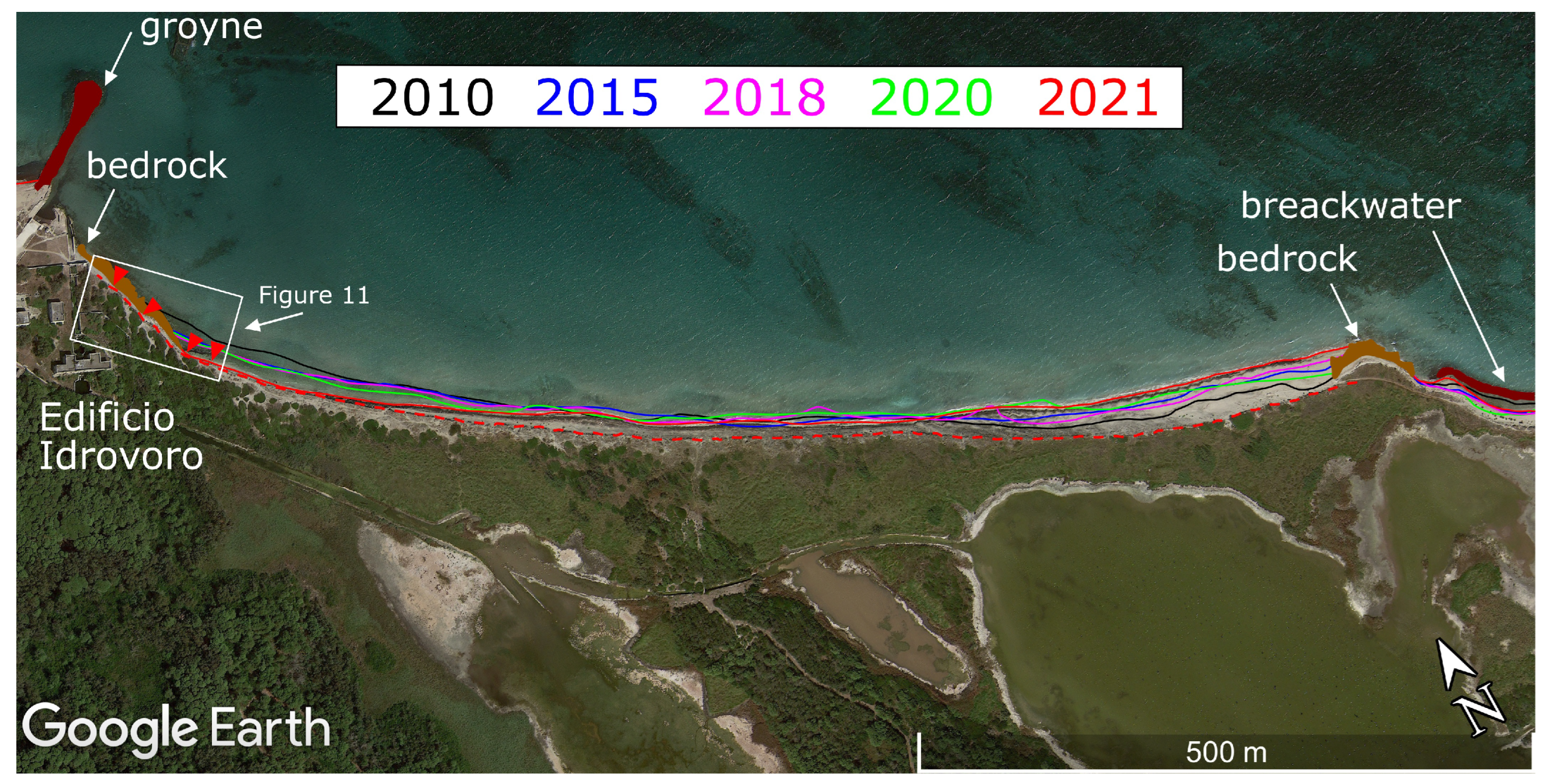
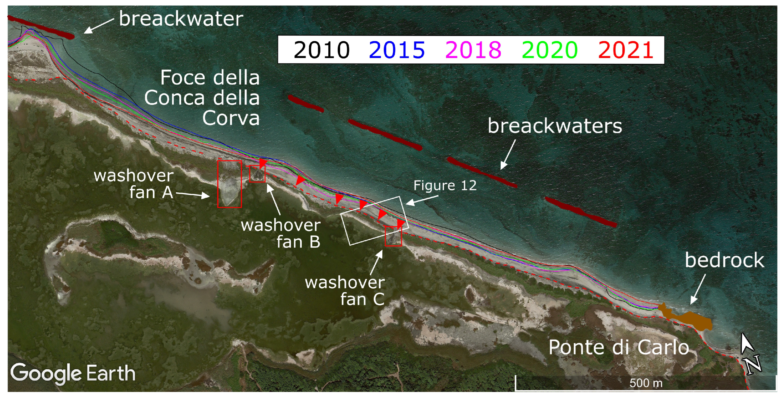
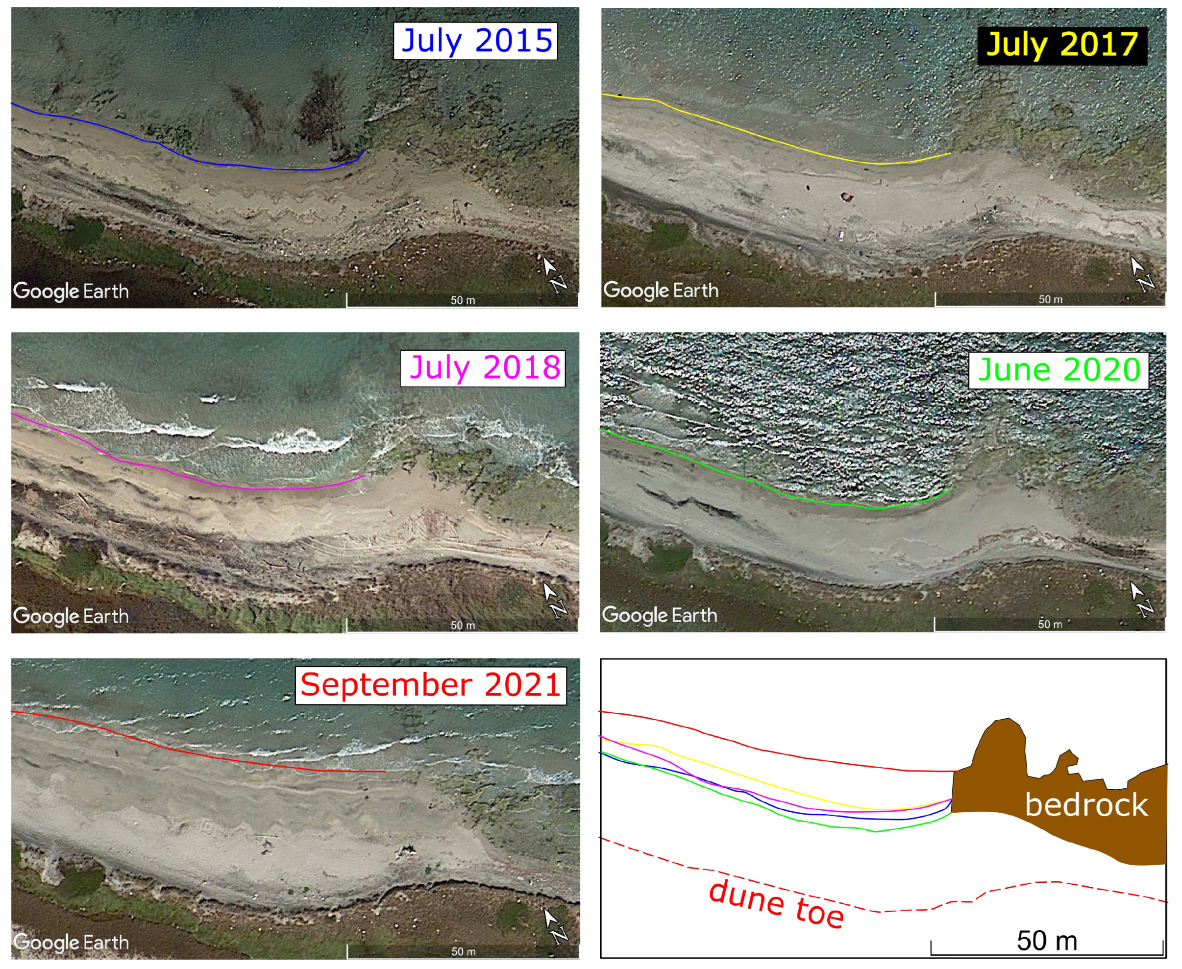
4.3. Instantaneous Shorelines Comparison
4.4. Geomorphological Changes
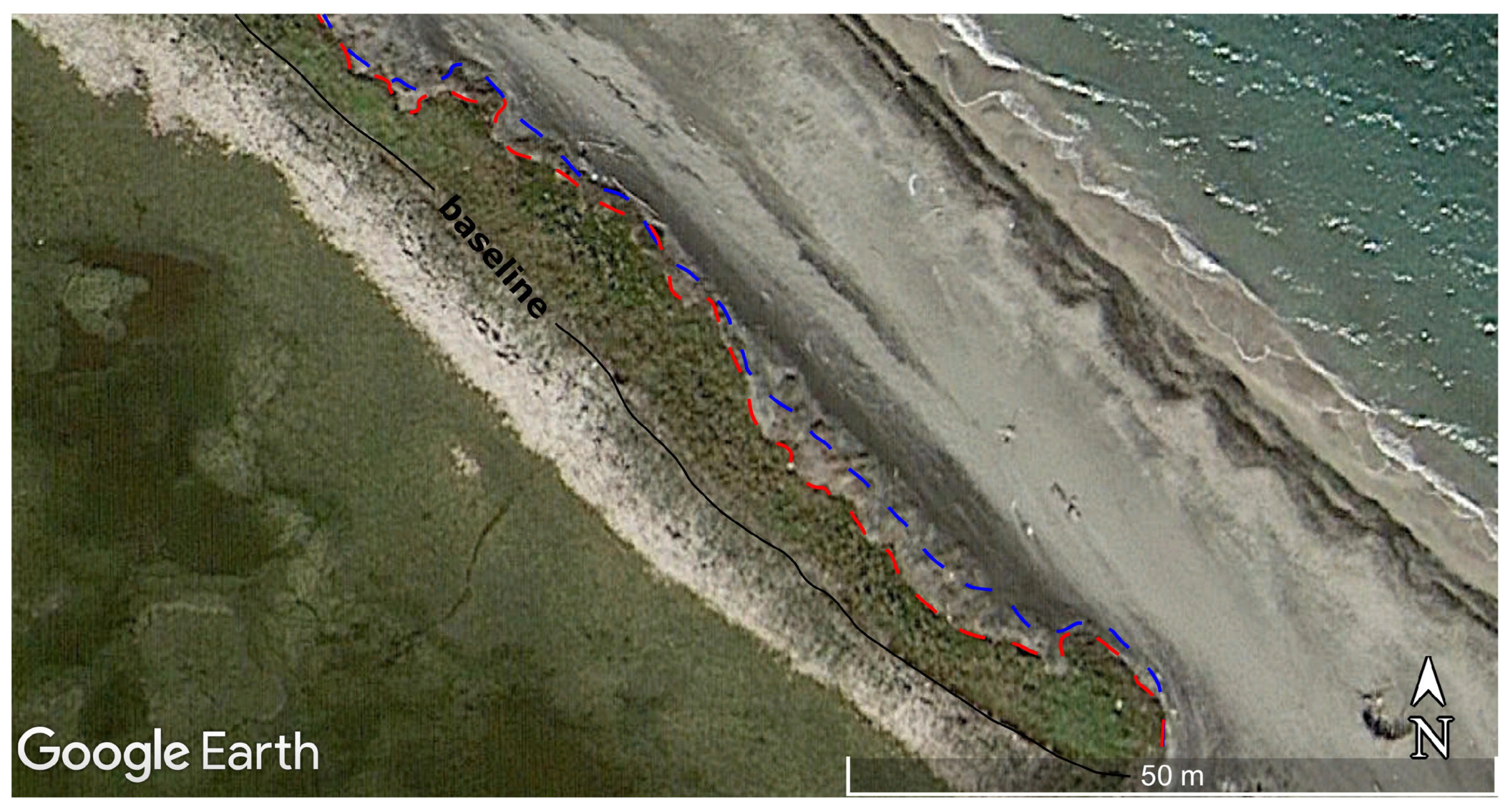
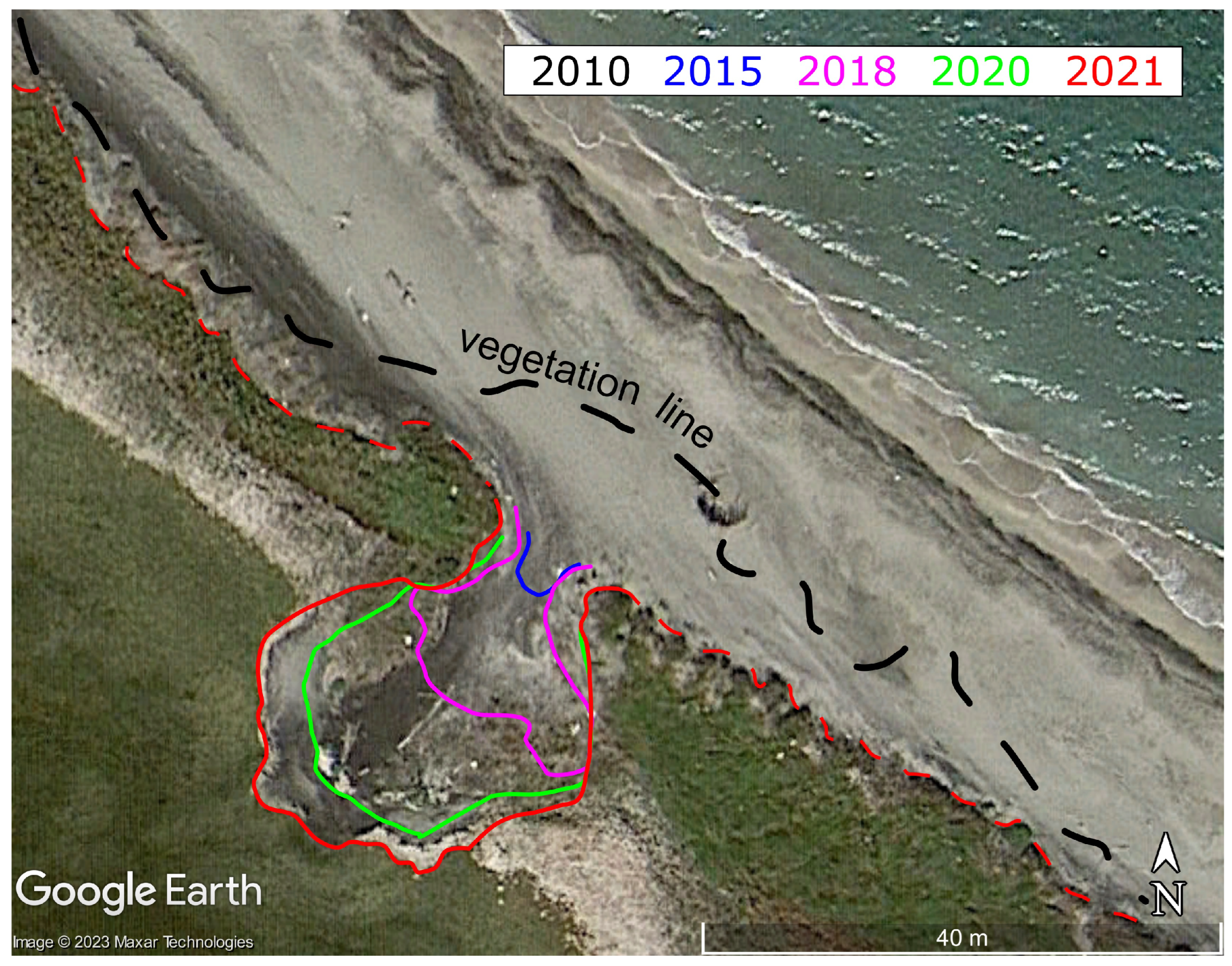
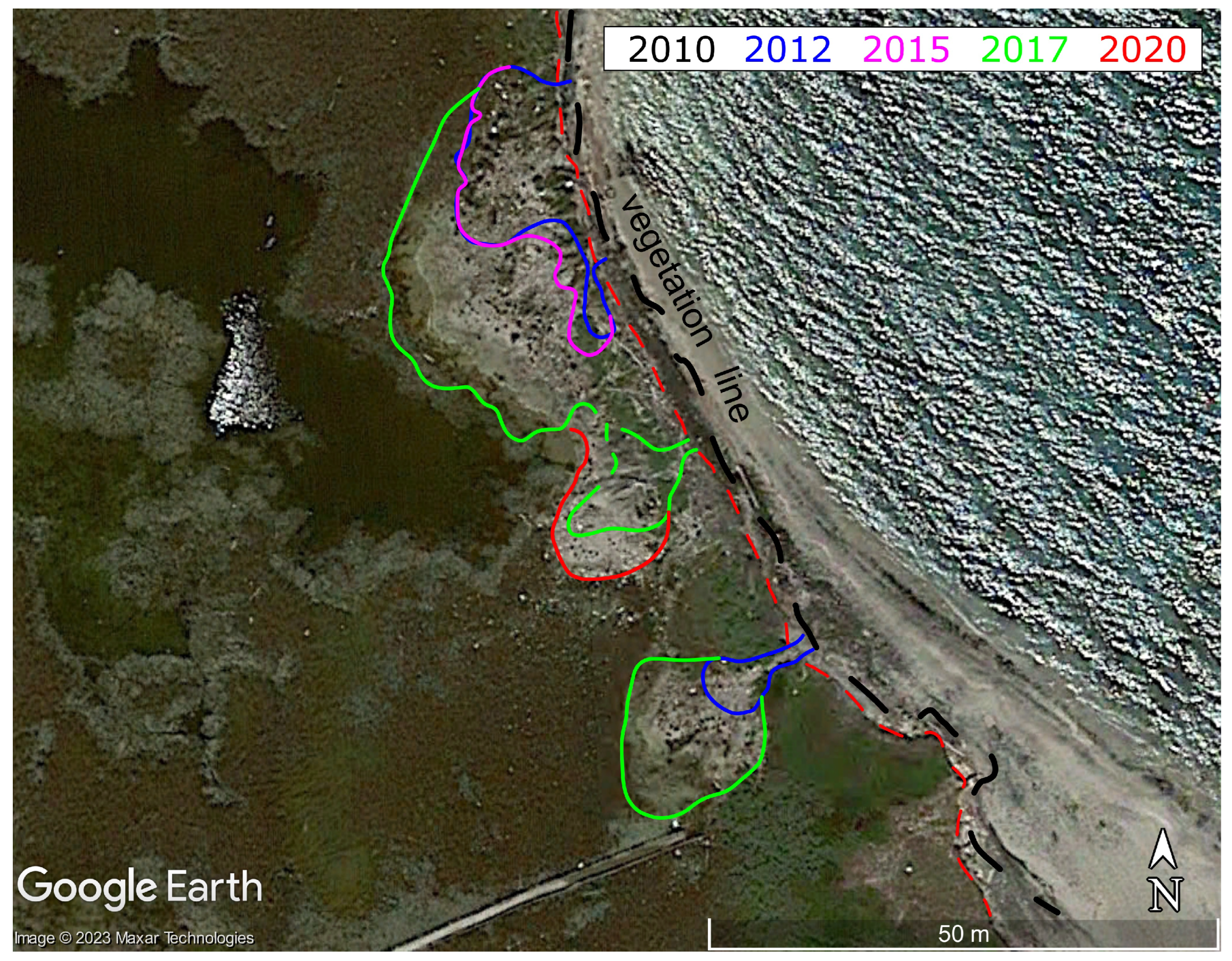
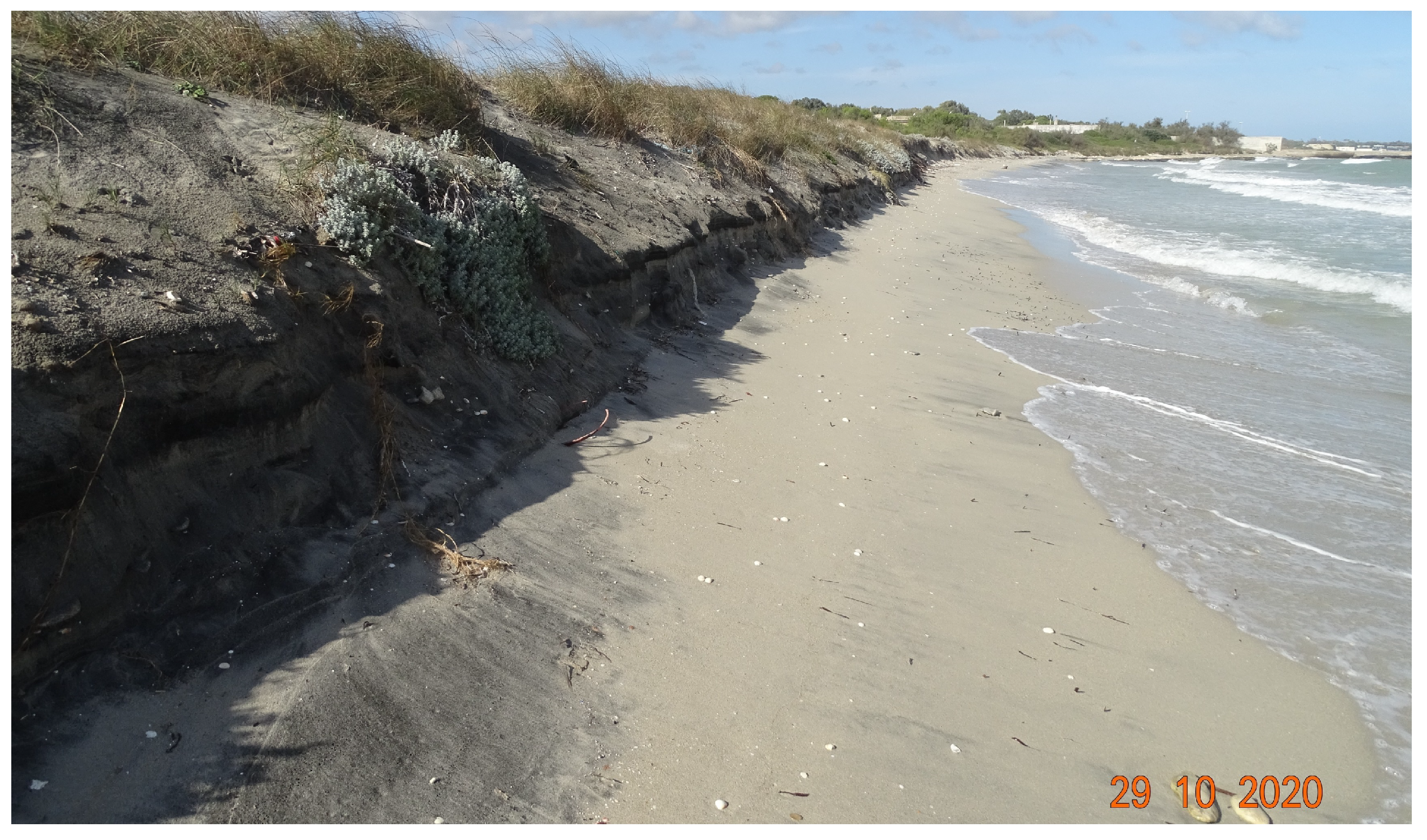
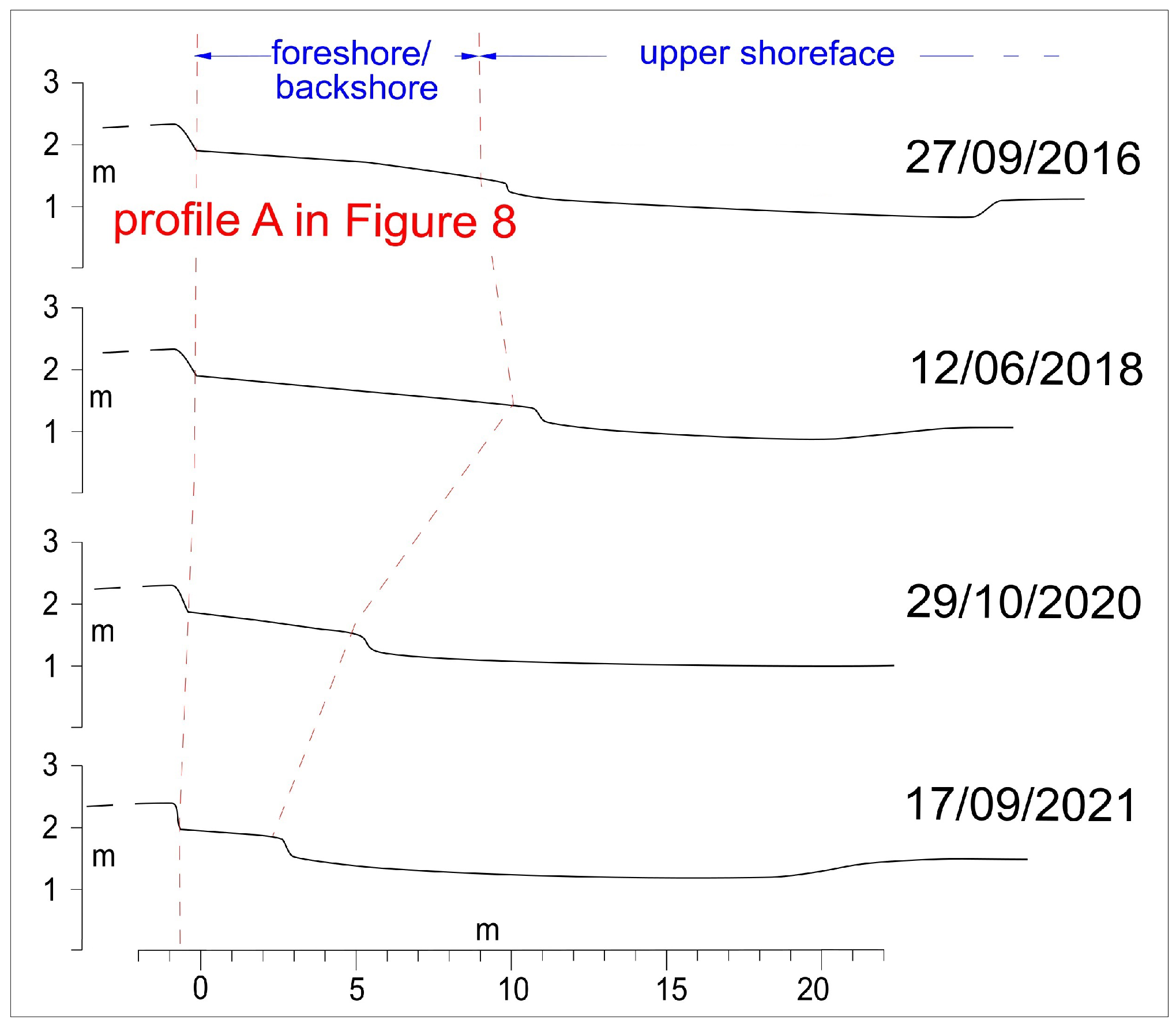
4.4.1. Dune Toe Retreat
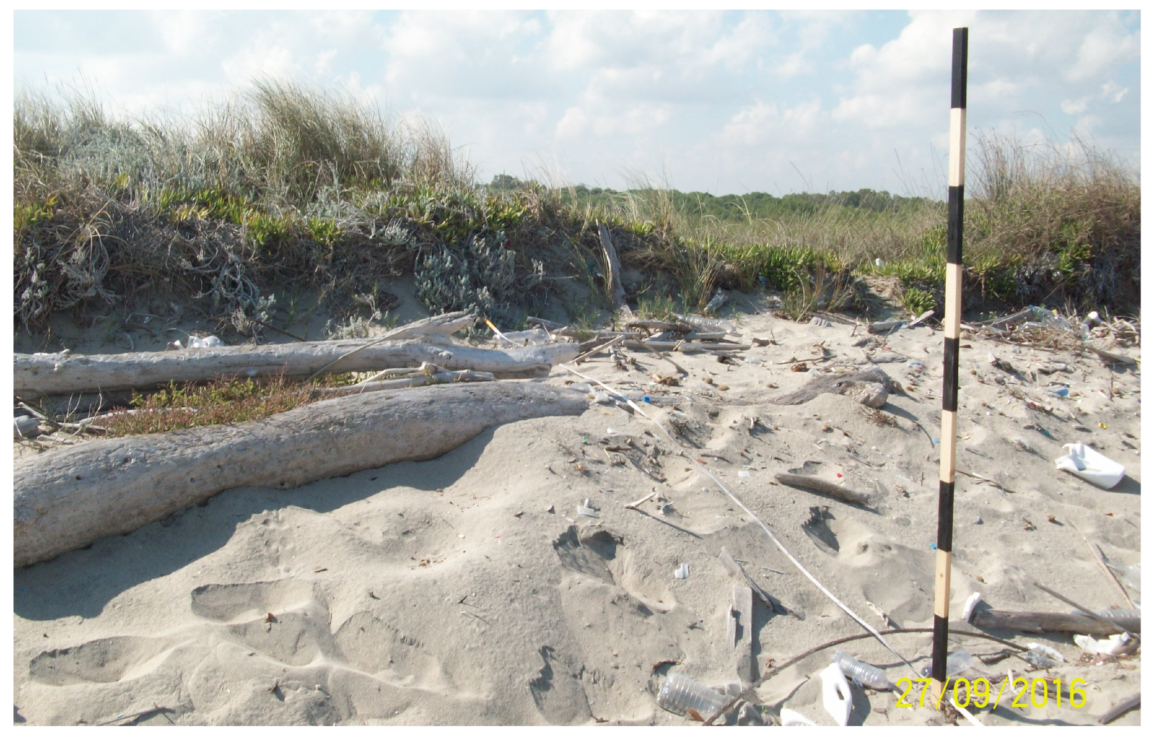
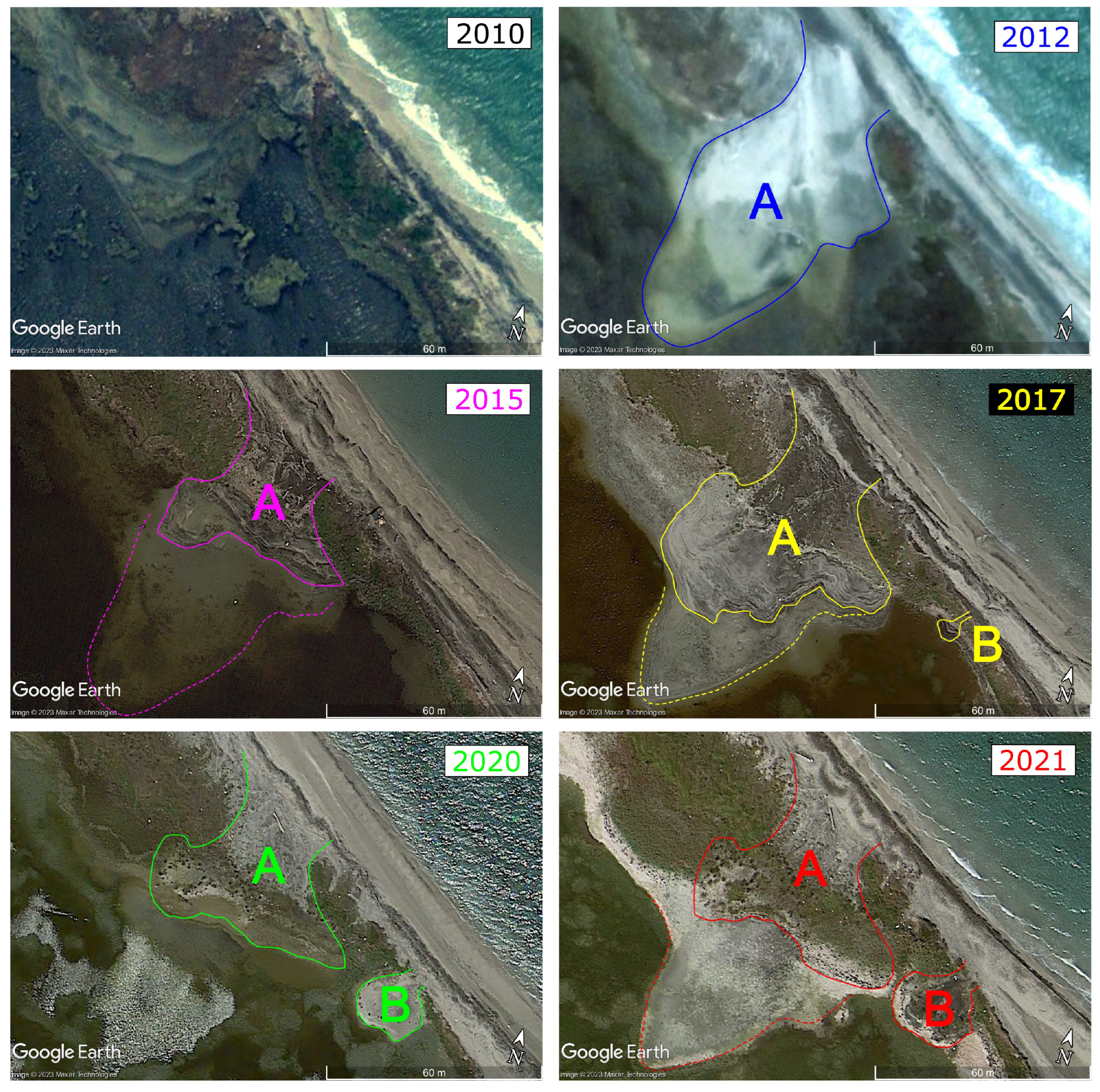
4.4.2. Washover Fan Accretion
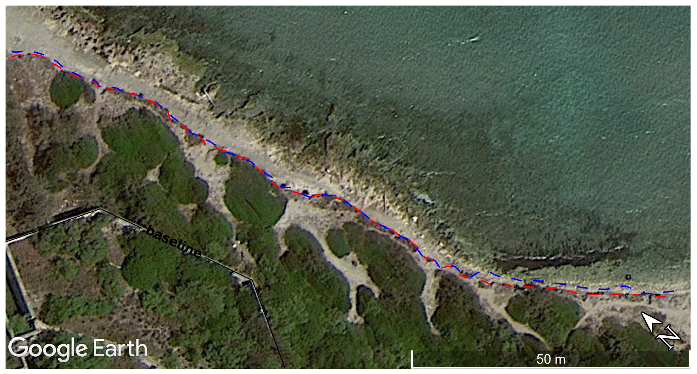
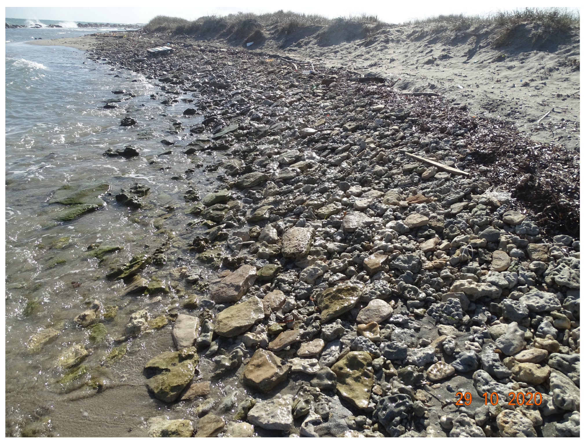
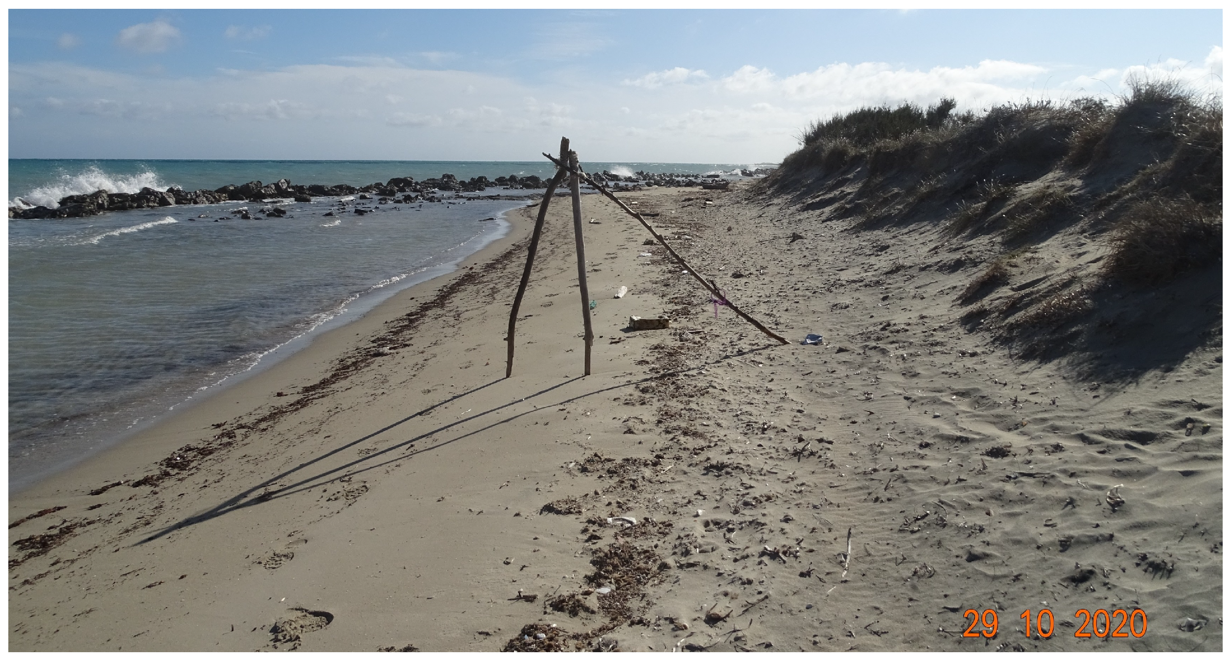
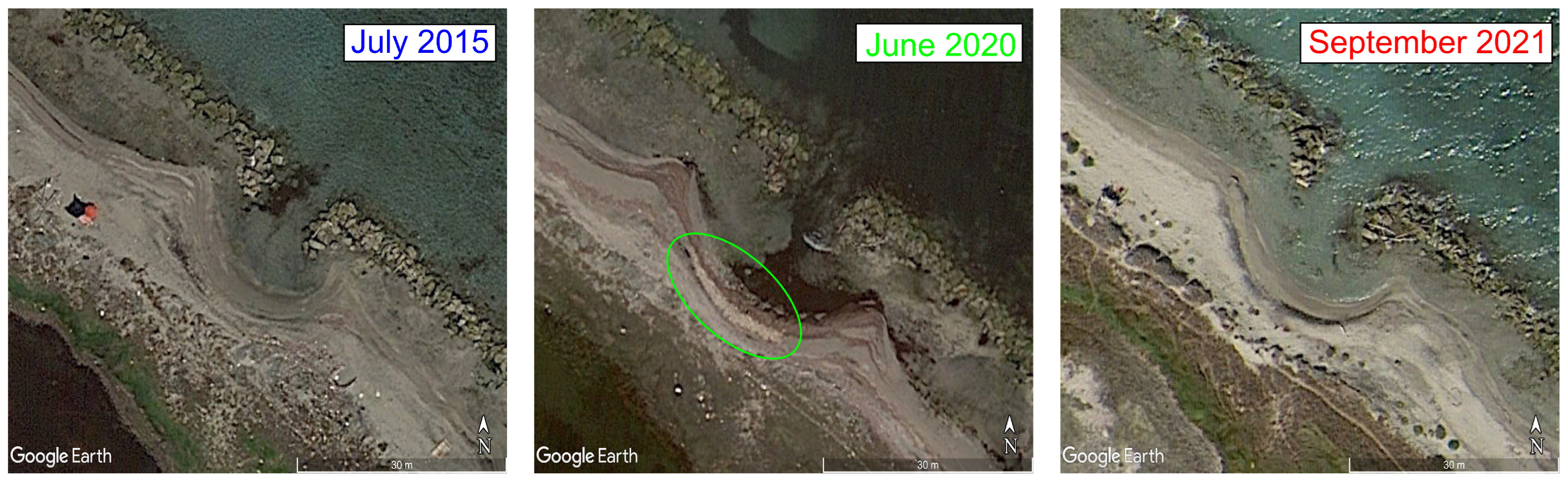
4.4.3. Gravel Beach Formation
5. Discussion and Conclusions
Author Contributions
Funding
Institutional Review Board Statement
Informed Consent Statement
Data Availability Statement
Acknowledgments
Conflicts of Interest
Sample Availability
Appendix A. Notes on Images Interpretation
Appendix B. Wind Rose and Speed Distribution


Appendix C. Grain Size Characterization

Appendix D. Additional Geomorphological Observations


References
- Leatherman, S.P. Barrier dune systems: A re-assessment. Sediment. Geol. 1979, 24, 1–16. [Google Scholar] [CrossRef]
- Morton, R.; Sallenger, A.H. Morphological impacts of extreme storms on sandy beaches and barriers. J. Coast. Res. 2003, 19, 560–573. [Google Scholar]
- Dillenburg, S.R.; Hesp, P.A. Coastal Barriers—An Introduction. In Geology and Geomorphology of Holocene Coastal Barriers of Brazil. Lecture Notes in Earth Sciences, Vol 107; Springer: Berlin/Heidelberg, Germany, 2009; pp. 1–15. [Google Scholar]
- Anthony, E.J.; Marriner, N.; Morhange, C. Human influence and the changing geomorphology of Mediterranean deltas and coasts over the last 6000 years: From progradation to destruction phase? Earth Sci. Rev. 2014, 139, 336–361. [Google Scholar] [CrossRef]
- Sherman, D.J.; Bauer, B.O. Coastal geomorphology through the looking glass. Geomorphology 1993, 7, 225–249. [Google Scholar] [CrossRef]
- Narayana, A.C. Shoreline Changes. In Encyclopedia of Estuaries. Encyclopedia of Earth Series; Kennish, M.J., Ed.; Springer: Dordrecht, The Netherlands, 2016; pp. 590–602. [Google Scholar]
- Kumar, A.; Jayappa, K.S. Long and short-term shoreline changes along Mangalore coast, India. Int. J. Environ. Res. 2009, 3, 177–188. [Google Scholar] [CrossRef]
- Rodriguez, A.B.; Theuerkauf, E.J.; Ridge, J.T.; VanDusen, B.M.; Fegley, S.R. Long-term washover fan accretion on a transgressive barrier island challenges the assumption that paleotempestites represent individual tropical cyclones. Sci. Rep. 2020, 10, 19755. [Google Scholar] [CrossRef]
- Santos, C.A.G.; do Nascimento, T.V.M.; Mishra, M.; da Silva, R.M. Analysis of long-and short-term shoreline change dynamics: A study case of Joao Pessoa city in Brazil. Sci. Total Environ. 2021, 769, 144889. [Google Scholar] [CrossRef]
- Brunel, C.; Sabatier, F. Potential influence of sea-level rise in controlling shoreline position on the French Mediterranean Coast. Geomorphology 2009, 107, 47–57. [Google Scholar] [CrossRef]
- El-Asmar, H.M.; El-Kafrawy, S.B.; Taha, M.M.N. Monitoring coastal changes along Damietta promontory and the barrier beach toward Port Said east of the Nile Delta, Egypt. J. Coast. Res. 2014, 30, 993–1005. [Google Scholar] [CrossRef]
- Delle Rose, M. Medium-term Erosion Processes of South Adriatic Beaches (Apulia, Italy): A Challenge for an Integrated Coastal Zone Management. J. Earth Sci. Clim. Chang. 2015, 6, 306. [Google Scholar] [CrossRef]
- Poulos, S.E.; Ghionis, G.; Verykiou, E.; Roussakis, G.; Sakellariou, D.; Karditsa, A.; Alexandrakis, G.; Petrakis, S.; Sifnioti, D.; Panagiotopoulos, I.P.; et al. Hydrodynamic, neotectonic and climatic control of the evolution of a barrier beach in the microtidal environment of the NE Ionian Sea (eastern Mediterranean). Geo-Mar. Lett. 2015, 35, 37–52. [Google Scholar] [CrossRef]
- Delle Rose, M. Studi per la previsione delle dinamiche evolutive della costa adriatica ad est di Lecce. Geol. e Terr. 2007, 4, 181–191. (In Italian) [Google Scholar]
- Lisi, I.; Bruschi, A.; Del Gizzo, M.; Archina, M.; Barbano, A.; Corsini, C. Physiographic units and depths of closure for the Italian coast. L’Acqua 2010, 2, 35–52. (In Italian) [Google Scholar]
- Tropeano, M.; Spalluto, L. Present-day temperate-type carbonate sedimentation on Apulian Shelves (southern Italy). GeoActs 2006, 5, 129–142. [Google Scholar]
- Mastronuzzi, G.; Sanso, P. Coastal towers and historical sea level change along the Salento coast (southern Apulia, Italy). Quatern. Int. 2014, 332, 61–72. [Google Scholar] [CrossRef]
- Margiotta, S.; Parise, M. Hydraulic and Geomorphological Hazards at Wetland Geosites Along the Eastern Coast of Salento (SE Italy). Geoheritage 2019, 11, 1655–1666. [Google Scholar] [CrossRef]
- De Giorgio, G.; Chieco, M.; Zuffianò, L.E.; Limoni, P.P.; Sottani, A.; Pedron, R.; Vettorello, L.; Stellato, L.; Di Rienzo, B.; Polemio, M. The Compatibility of Geothermal Power Plants with Groundwater Dependent Ecosystems: The Case of the Cesine Wetland (Southern Italy). Sustainability 2018, 10, 303. [Google Scholar] [CrossRef]
- Medagli, P.; Sciandrello, S.; Mele, C.; Di Pietro, R.; Wagensommer, R.P.; Urbano, M.; Tomaselli, V. Analisi della biodiversità vegetale e cartografia della vegetazione, degli habitat e dell’uso del suolo della Riserva Naturale Statale “Le Cesine” (Lecce—Puglia). Quat. Bot. Amb. Appl. 2013, 24, 55–76. (In Italian) [Google Scholar]
- Tomaselli, V.; Veronico, G.; Adamo, M. Monitoring and Recording Changes in Natural Landscapes: A Case Study from Two Coastal Wetlands in SE Italy. Land 2021, 10, 50. [Google Scholar] [CrossRef]
- Delle Rose, M.; Beccarisi, L.; Elia, T. Short-medium term assessments of coastal erosion and marine inundation effects on natural and anthropic environments (Apulia, Southern Italy). In Marine Research at CNR, Coastal and Marine and Spatial Planing; Brugnoli, E., Cavarretta, G., Mazzola, S., Trincardi, F., Ravaioli, M., Santoleri, R., Eds.; National Research Council: Rome, Italy, 2011; pp. 1149–1163. Available online: https://dta.cnr.it/category/marine-research-at-cnr/ (accessed on 15 March 2023).
- Delle Rose, M.; Parise, M. Karst subsidence in South-Central Apulia, Southern Italy. Int. J. Speleol. 2002, 31, 181–199. [Google Scholar] [CrossRef]
- Caldara, M.; Centenaro, E.; Mastronuzzi, G.; Sanso, P.; Sergio, A. Features and Present Evolution of Apulian Coast (Southern Italy). In Proceedings of the 5th International Coastal Symposium, Palm Beach, FL, USA, 19–23 May 1998. J. Coast. Res., spec. issue 26, 1999, pp. 55–64. [Google Scholar]
- Dominici, R.; Donato, P.; Basta, P.; Romano, G.; Delle Rose, M.; Tenuta, M.; Vacca, C.; Verrino, M.; De Rosa, R. Mineralogical and textural characterization of the Alimini beach sands: Implication on their provenance and transport processes. Rend. Online Soc. Geol. It. 2016, 38, 39–42. [Google Scholar] [CrossRef]
- Boenzi, F.; Caldara, M.; Pennetta, L.; Simone, O. Environmental Aspects Related to the Physical Evolution of Some Wetlands Along the Adriatic Coast of Apulia (Southern Italy): A Review. In Proceedings of the 8th International Coastal Symposium, Itajai, Brazil, 14–19 March 2004. J. Coast. Res., spec. issue 39, 2006, pp. 170–175. [Google Scholar]
- Guglielmino, A.; Buckle, C. Remarks on the composition of the Auchenorrhyncha fauna in some moist areas in Southern Apulia (Italy). Biodivers. J. 2015, 6, 309–322. [Google Scholar]
- National Geoportal. Available online: http://www.pcn.minambiente.it/mattm/en/ (accessed on 13 February 2023).
- Spano, D.; Snyder, R.L.; Cesaraccio, C. Mediterranean Climates. In Phenology: An Integrative Environmental Science; Schwartz, M.D., Ed.; Springer: Dordrecht, The Netherlands, 2003; pp. 139–156. [Google Scholar]
- Lionello, P.; Malanotte-Rizzoli, P.; Boscolo, R.; Alpert, P.; Artale, V.; Li, L.; Luterbacher, J.; May, W.; Trigo, R.; Tsimplis, M.; et al. The Mediterranean Climate: An Overview of the Main Characteristics and Issues. Dev. Earth Environ. Sci. 2006, 4, 1–26. [Google Scholar]
- Zito, G.; Ruggiero, L.; Zuanni, F. Aspetti meteorologici e climatici della Puglia. In Proceedings of the First Workshop on “Clima, Ambiente e Territorio nel Mezzogiorno”, Taormina, Italy, 11–12 December 1989; CNR: Roma, Italy, 1991; pp. 43–73. (In Italian). [Google Scholar]
- Ruol, P.; Martinelli, L.; Favaretto, C.; Barbariol, F.; Benetazzo, A. Representative and Morphological Waves along the Adriatic Italian Coast in a Changing Climate. Water 2022, 14, 2678. [Google Scholar] [CrossRef]
- Caloiero, T.; Aristodemo, F. Trend Detection of Wave Parameters along the Italian Seas. Water 2021, 13, 1634. [Google Scholar] [CrossRef]
- Poulain, P.M. Adriatic Sea surface circulation as derived from drifter data between 1990 and 1999. J. Mar. Syst. 2001, 29, 3–32. [Google Scholar] [CrossRef]
- Kalimeris, A.; Kassis, D. Sea surface circulation variability in the Ionian-Adriatic Seas. Prog. Oceanogr. 2020, 189, 102454. [Google Scholar] [CrossRef]
- Rete Mareografica Nazionale. Available online: https://www.mareografico.it/ (accessed on 20 February 2023).
- Benetazzo, A.; Fedele, F.; Carniel, S.; Ricchi, A.; Bucchignani, E.; Sclavo, M. Wave climate of the Adriatic Sea: A future scenario simulation. Nat. Hazards Earth Syst. Sci. 2012, 12, 2065–2076. [Google Scholar] [CrossRef]
- Mikulic, A.; Parunov, J. A Wave Directionality and a Within-Year Wave Climate Variability Effects on the Long-Term Extreme Significant Wave Heights Prediction in the Adriatic Sea. J. Mar. Sci. Eng. 2023, 11, 42. [Google Scholar] [CrossRef]
- Sartini, L.; Cassola, F.; Besio, G. Extreme waves seasonality analysis: An application in the Mediterranean Sea. J. Geophys. Res. Oceans 2015, 120, 6266–6288. [Google Scholar] [CrossRef]
- SIMOP, Sistema Informativo Meteo Oceanografico delle coste Pugliesi, Autorità di Bacino della Puglia. Available online: http://93.51.158.171/web/simop/home (accessed on 20 January 2023).
- Regione Puglia. Annali Idrologici. 2015. Available online: https://protezionecivile.puglia.it/documents/3171874/3243680/annale2015.pdf/ (accessed on 30 December 2022). (In Italian).
- Regione Puglia. Annali Idrologici. 2016. Available online: https://protezionecivile.puglia.it/documents/3171874/3243680/annale2016.pdf/ (accessed on 30 December 2022). (In Italian).
- Regione Puglia. Annali Idrologici. 2017. Available online: https://protezionecivile.puglia.it/documents/3171874/3243680/annale2017.pdf/ (accessed on 30 December 2022). (In Italian).
- Regione Puglia. Annali Idrologici. 2018. Available online: https://protezionecivile.puglia.it/documents/3171874/3243680/annale2018.pdf/ (accessed on 30 December 2022). (In Italian).
- Regione Puglia. Annali Idrologici. 2019. Available online: https://protezionecivile.puglia.it/documents/3171874/3243680/annale2019.pdf/ (accessed on 30 December 2022). (In Italian).
- Regione Puglia. Annali Idrologici. 2020. Available online: https://protezionecivile.puglia.it/documents/3171874/3243680/annale2020rev2.pdf/ (accessed on 30 December 2022). (In Italian).
- Regione Puglia. Annali Idrologici. 2021. Available online: https://protezionecivile.puglia.it/documents/3171874/3243680/annale2021.pdf/ (accessed on 30 December 2022). (In Italian).
- Shu, Z.R.; Jesson, M. Estimation of Weibull parameters for wind energy analysis across the UK. J. Renew. Sustain. Energy 2021, 13, 023303. [Google Scholar] [CrossRef]
- Harley, M. Coastal Storm Definition. In Coastal Storms; Ciavola, P., Coco, G., Eds.; John Wiley & Sons: Hoboken, NJ, USA, 2017; pp. 1–21. [Google Scholar]
- Boccotti, P. Wave Mechanics for Ocean Engineering; Elsevier Science: Amsterdam, The Netherlands, 2000; pp. 1–496. [Google Scholar]
- BOLAM-MOLOCH Forecasts. Available online: http://www.isac.cnr.it/dinamica/projects/forecasts/index.html (accessed on 28 March 2023).
- Hsu, S.A. (Ed.) Coastal Meteorology; Academic Press: Cambridge, MA, USA, 1988; 260p. [Google Scholar]
- Delle Rose, M.; Martano, P.; Orlanducci, L. Coastal Boulder Dynamics Inferred from Multi-Temporal Satellite Imagery, Geological and Meteorological Investigations in Southern Apulia, Italy. Water 2021, 13, 2426. [Google Scholar] [CrossRef]
- Gill, A. Atmosphere-Ocean Dynamics, 1st ed.; Academic Press: London, UK, 1982; p. 662. [Google Scholar]
- Delgado, I.; Lloyd, G. A simple low cost method for one person beach Profiling. J. Coastal. Res. 2004, 20, 1246–1252. [Google Scholar] [CrossRef]
- Osborne, P.D. Cross-shore variation of grain size on beaches. In Encyclopedia of Coastal Science: Encyclopedia of Earth Sciences Series; Finkl, C., Makowski, C., Eds.; Springer: Cham, Switzerland, 2018; pp. 313–319. [Google Scholar]
- Blaschke, T.; Hay, G.J.; Kelly, M.; Lang, S.; Hofmann, P.; Addink, E.; Queiroz Feitosa, R.; van der Merr, F.; van der Werff, H.; van Coillie, F.; et al. Geographic Object-Based Image Analysis—Towards a new paradigm. J. Photogramm. Remote Sens. 2014, 87, 180–191. [Google Scholar] [CrossRef] [PubMed]
- Chen, G.; Weng, Q.; Hay, G.J.; He, Y. Geographic object-based image analysis (GEOBIA): Emerging trends and future opportunities. GIScience Remote Sens. 2018, 55, 159–182. [Google Scholar] [CrossRef]
- Boak, E.H.; Turner, I.L. Shoreline Definition and Detection: A Review. J. Coast. Res. 2005, 21, 688–703. [Google Scholar] [CrossRef]
- Lee, I.C. Instantaneous shoreline mapping from worldview-2 satellite images by using shadow analysis and spectrum matching techniques. J. Environ. Sci. Technol. 2016, 24, 1204–1216. [Google Scholar]
- Dang, Y.; Zhang, C.; Zhou, X.; Xu, J.; Xue, S. Instantaneous shorelines as an intermediate for island shoreline mapping based on aerial/satellite stereo images. Mar. Geod. 2018, 41, 219–229. [Google Scholar] [CrossRef]
- Vos, K.; Harley, M.D.; Splinter, K.D.; Simmons, J.A.; Turner, I.L. Sub-annual to multi decadal shoreline variability from publicly available satellite imagery. Coast. Eng. 2019, 150, 160–174. [Google Scholar] [CrossRef]
- Jia, P.; Zhang, Y.; Xu, W.; Xia, Z.; Zhong, C.; Yin, Y. Spatio-temporal evolution of coastline of sand-barrier lagoons over 26 years through historic Landsat imagery in Lingshui County, Hainan Province, China. J. Coast. Conserv. 2019, 23, 817–827. [Google Scholar] [CrossRef]
- Splinter, K.D.; Kearney, E.T.; Turner, I.L. Driver of alongshore variable dune erosion during a storm event: Observation and modelling. Coast. Eng. 2018, 131, 31–41. [Google Scholar] [CrossRef]
- Van IJzendoorn, C.O.; de Vries, S.; Hallin, C.; Hesp, P.A. Sea level rise outpaced by vertical dune toe translation on prograding coasts. Sci. Rep. 2021, 11, 12792. [Google Scholar] [CrossRef]
- Kochel, R.C.; Laura, A.W. Relative Role of Overwash and Aeolian Processes on Washover Fans, Assateague Island, Virginia-Maryland. J. Coast. Res. 1989, 5, 453–475. [Google Scholar]
- Lorenzo-Trueba, J.; Ashton, A.D. Rollover, drowning, and discontinuous retreat: Distinct modes of barrier response to sea-level rise arising from a simple morphodynamic model. J. Geophys. Res. Earth Surf. 2014, 119, 779–801. [Google Scholar] [CrossRef]
- Simpson, D.P. Gravel Beaches. In Encyclopedia of Coastal Science. Encyclopedia of Earth Science Series; Schwartz, M.L., Ed.; Springer: Dordrecht, The Netherlands, 2005; pp. 492–494. [Google Scholar]
- Buscombe, D.; Masselink, G. Concepts in gravel beach dynamics. Earth Sci. Rev. 2006, 79, 33–52. [Google Scholar] [CrossRef]
- Filippaki, E.; Tsakalos, E.; Kazantzaki, M.; Bassiakos, Y. Forecasting Impacts on Vulnerable Shorelines: Vulnerability Assessment along the Coastal Zone of Messolonghi Area—Western Greece. Climate 2023, 11, 24. [Google Scholar] [CrossRef]
- Lapietra, I.; Lisco, S.; Capozzoli, L.; De Giosa, F.; Mastronuzzi, G.; Mele, D.; Milli, S.; Romano, G.; Sabatier, F.; Scardino, G.; et al. A Potential Beach Monitoring Based on Integrated Methods. J. Mar. Sci. Eng. 2022, 10, 1949. [Google Scholar] [CrossRef]
- Gracia, V.; García, M.; Grifoll, M.; Sánchez-Arcilla, A. Breaching of a barrier beach under extreme events. The role of morphodynamic simulations. In Proceedings of the 12th International Coastal Symposium, Plymouth, UK, 9–13 April 2013. J. Coast. Res., spec. issue 65, 2013, pp. 951–956. [Google Scholar]
- Gallop, S.L.; Harley, M.D.; Brander, R.W.; Simmons, J.A.; Splinter, K.D.; Turner, I.L. Assessing Cross-Shore and Alongshore Variation in Beach Morphology Due to Wave Climate: Storms to Decades. Oceanography 2017, 30, 120–125. [Google Scholar] [CrossRef]
- Foti, G.; Barbaro, G.; Barilla, G.C.; Mancuso, P.; Puntorieri, P. Shoreline Evolutionary Trends Along Calabrian Coasts: Causes and Classification. Front. Mar. Sci. 2022, 9, 846914. [Google Scholar] [CrossRef]
- Roca, M.; Navarro, G.; García-Sanabria, J.; Caballero, I. Monitoring Sand Spit Variability Using Sentinel-2 and Google Earth Engine in a Mediterranean Estuary. Remote Sens. 2022, 14, 2345. [Google Scholar] [CrossRef]
- Wentworth, C.K. A Scale of Grade and Class Terms for Clastic Sediments. J. Geol. 1922, 30, 377–392. [Google Scholar] [CrossRef]
- Krumbein, W.C. Size frequency distributions of sediments. J. Sediment. Petrol. 1934, 4, 65–77. [Google Scholar] [CrossRef]
- Blott, S.J.; Pye, K. Particle size scales and classification of sediment types based on particle size distributions: Review and recommended procedures. Sedimentology 2012, 59, 2071–2096. [Google Scholar] [CrossRef]


| Season/Sector | Vm | V (0.25) | V (0.50) | V (0.75) | 1Y v (min–max) | 1Y U (min–max) | 1Y H (min–max) |
|---|---|---|---|---|---|---|---|
| CW-N | 0.8 | 3.7 | 2.1 | 1.0 | 9.0–11.6 | 16–20 | 3.7–5.6 |
| CW-E | 1.6 | 2.8 | 2.0 | 1.2 | 5.6–6.2 | 15–17 | 3.4–4.2 |
| CW-S | 2.9 | 3.8 | 3.0 | 2.2 | 6.0–6.8 | 16–20 | 5.8–7.2 |
| WD-N | 2.3 | 3.7 | 2.7 | 1.7 | 7.0–7.7 | 12–15 | 3.4–4.8 |
| WD-E | 2.0 | 2.5 | 2.0 | 1.5 | 4.2–4.3 | 10–10 | 2.3–3.2 |
| WD-S | 3.3 | 4.0 | 3.3 | 2.6 | 5.0–5.6 | 8–15 | 2.4–5.4 |
Disclaimer/Publisher’s Note: The statements, opinions and data contained in all publications are solely those of the individual author(s) and contributor(s) and not of MDPI and/or the editor(s). MDPI and/or the editor(s) disclaim responsibility for any injury to people or property resulting from any ideas, methods, instructions or products referred to in the content. |
© 2023 by the authors. Licensee MDPI, Basel, Switzerland. This article is an open access article distributed under the terms and conditions of the Creative Commons Attribution (CC BY) license (https://creativecommons.org/licenses/by/4.0/).
Share and Cite
Delle Rose, M.; Martano, P. Wind–Wave Conditions and Change in Coastal Landforms at the Beach–Dune Barrier of Cesine Lagoon (South Italy). Climate 2023, 11, 128. https://doi.org/10.3390/cli11060128
Delle Rose M, Martano P. Wind–Wave Conditions and Change in Coastal Landforms at the Beach–Dune Barrier of Cesine Lagoon (South Italy). Climate. 2023; 11(6):128. https://doi.org/10.3390/cli11060128
Chicago/Turabian StyleDelle Rose, Marco, and Paolo Martano. 2023. "Wind–Wave Conditions and Change in Coastal Landforms at the Beach–Dune Barrier of Cesine Lagoon (South Italy)" Climate 11, no. 6: 128. https://doi.org/10.3390/cli11060128
APA StyleDelle Rose, M., & Martano, P. (2023). Wind–Wave Conditions and Change in Coastal Landforms at the Beach–Dune Barrier of Cesine Lagoon (South Italy). Climate, 11(6), 128. https://doi.org/10.3390/cli11060128