Application of Hydrological Modeling Related to the 2011 Disaster in the Mountainous Region of Rio De Janeiro, Brazil

Abstract

Natural disasters have been responsible for thousands of deaths in recent decades that, added to the environmental, social and economic impacts, require the implementation of prevention strategies. The largest share of disasters is of hydrological origin. In this context, hydrological models are potential alternatives for monitoring and preventing events of this nature. The objective of this study was to analyze the applicability of the semi-distributed model SWAT (Soil and Water Assessment Tool) and the concentrated model SMAP (soil moisture accounting procedure) in predicting the extreme flood event that occurred in Brazil in the mountainous region of Rio de Janeiro in 2011. The results showed that the mean relative error in calibration and validation was 12% and 53% for SMAP, and 18.46% and 88.73% for SWAT, respectively. The better performance of SMAP in validation integrated with its ease of data collection, simplicity of execution and semi-automatic calibration included in its routine, allows for the conclusion that this model proved to be more suitable for hydrological monitoring. In this study, for the first time, a model of SWAT’s complexity was applied to a watershed located in the mountainous region of the state of Rio de Janeiro, a region that, unfortunately, has accounted for thousands of deaths over the past decades associated with mass movements and floods. The SWAT model, besides being able to predict the level and flow of the main course of the river and its tributaries, also enables the calculation of sediment transport in extreme events. Looking from an operational point of view, the work clearly shows how poor hydro-meteorological monitoring, as is the case in this region, makes a good quality prediction for extreme events impossible. It was demonstrated that under these conditions, a simpler and concentrated modeling approach, such as the SMAP model, is able to obtain better results than SWAT.

1. Introduction

Natural disasters have been highlighted by the severity of the impacts generated in society, the environment and the countless lives lost where they occur. The disasters were responsible for 3.3 million deaths in 40 years of records [1] These events affected an annual average of 193.4 million people for the period between 2001 and 2021. Events of hydrological origin (floods and landslides) configure the largest share of disasters affecting the world population [2]. In Brazil, drought is the event of highest incidence, followed, respectively, by torrents and floods [3].

The natural disaster that occurred in 2011 in the mountainous region of Rio de Janeiro, Brazil, was the worst event in the country. As a result, new instruments and guidelines were created to deal with natural disasters established by Law No. 12608/2012 [4]. However, despite this progress, disasters continue to impact countless lives in this same region, where fatalities were recorded again due to heavy rains in 2022.

The need to reduce the impacts of disasters, whose incidence has become more recurrent, leads to the search for the reduction of vulnerability and exposure of the system to risks, not only with the adoption of structural but also non-structural measures, aimed at increasing the perception of and resilience to these events [5,6].

The monitoring and prognoses of these events are essential to prevent possible impacts and, mainly, to avoid potential fatalities. In this sense, mathematical hydrological models can be a viable alternative for monitoring the forecast of flood flows from a given precipitation, in order to alert the population and civil defense to take preventive measures [7].

Hydrological models have been developed for various purposes, initially for quantitative purposes. Afterwards, environmental issues and the evaluation of the impacts of land use led to the development of new models, based on physical laws, modeling in a distributed manner, aiming, in addition to the prediction of flow, qualitative analyses and studies of alternative scenarios. However, the distributed models do not necessarily generate better results than the concentrated ones, often justified by difficulty of model adjustment, due to the expressive number of parameters, and the lack of spatial and temporal representativeness of rainfall data from the basin [8].

In this context, the semi-distributed hydrological model Soil and Water Assessment Tool (SWAT), characterized by simulations in large watersheds, stands out with regard to plant growth, nutrient and chemical movements, erosion processes, agricultural activities, good management practices, alternative scenario generation, and climate customization [9]. This diversity of functionality provides a wide variety of applications, initially focused on issues related to diffuse sources of pollution, management impacts on water resources, sediment production, and agricultural chemical spread, and currently, expanded to climate change, water quality, bioenergy, and land use studies [10,11,12,13,14].

Of equal relevance, the concentrated soil moisture accounting procedure (SMAP) model, based on the principle of calculating flow as a function of rainfall, is characterized by simplification by representing the system from few parameters, governed by mass conservation and transfer functions in linear reservoirs [15,16].

Therefore, the present work aimed to analyze the potentiality of SWAT and SMAP models in predicting the extreme flood event that occurred in 2011 in the Rio Grande Basin, located in the municipalities of Nova Friburgo and Bom Jardim, in the state of Rio de Janeiro (RJ). In order to test the viability of these models as warning and monitoring systems for natural disasters, the study focused on the hydrological simulation performed with the SWAT model for further comparison with the study developed with the application of the SMAP model [17].

2. Materials and Methods

2.1. Study Area

The watershed under study is located on the meridians 42°43′ W and 42°24′ W and parallels 22°6′ S and 22°24′ S, corresponding to the upper course of the Rio Grande Basin (RJ) (Figure 1), with an area of approximately 558 km² and maximum elevation of 2261 m.

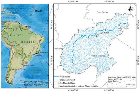
Figure 1. Map of location of the study basin—Upper Rio Grande Basin, RJ.

This region is characterized by the predominance of thick and leached soils, and by the humid and mild climate under the influence of orographic effects [18]. The climate is mesothermal, with rainy summers (moderately hot) and dry winters of the Cwb type (Köppen–Geiger classification) [19], as seen in Figure 2. The total annual precipitation corresponds to 1500 mm and the average annual temperature of 18 °C; the highest temperature occurs in the month of January [19].

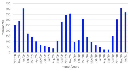
Figure 2. Total accumulated monthly precipitation for the period between 2008 and 2011 in the study area. The data from January 2011 represent the accumulated precipitation up to the 15th of this month, due to the destruction of stations in the event.

Due to the climatic and relief characteristics, the vegetation type is dense montana ombrophilous forest [20]. This coverage makes up the largest portion of the basin, followed by pastures and, finally, the urban areas that are not very expressive, concentrated in the eastern portion of Nova Friburgo.

2.2. The Natural Disaster in the Mountainous Region of Rio de Janeiro in 2011

On 11 and 12 January 2011, the mountainous region of the Rio de Janeiro, Brazil, suffered one of the country’s biggest disasters that caused about 905 deaths, 300 missing and affected more than 300,000 people [21,22].

The event marked by floods and landslides was the result of a set of climatic factors and local physical characteristics, as well as, land use and coverage, topography, and previous rainfall resulting from the establishment of the South Atlantic Convergence Zones (SACZ) over the region [21].

The rainfall rates in the disaster period were above normal, Figure 3; the Ypu, Sítio Santa Paula, Olaria and Nova Friburgo stations operated by the State Environment Institute (INEA) recorded, respectively, the accumulated totals of 222.8 mm, 240 mm, 241.8 mm and 182 mm in 24 h [21,22,23].

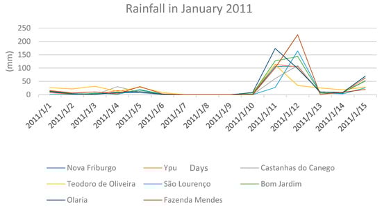
Figure 3. Daily precipitation at the stations in the Upper Rio Grande Basin, RJ.

On 11 January, the rains began calmly in the morning and throughout the day, triggering at 21 h the increase in rainfall intensity (strong to moderate) that lasted for eight consecutive hours [24]. On this day, the spatial variation of precipitation observed in the basin under study showed accumulated values of 20 to 180 mm/24 h (Figure 4) [24]. These values exceed 70% of the historical average observed for the month in the region [21].

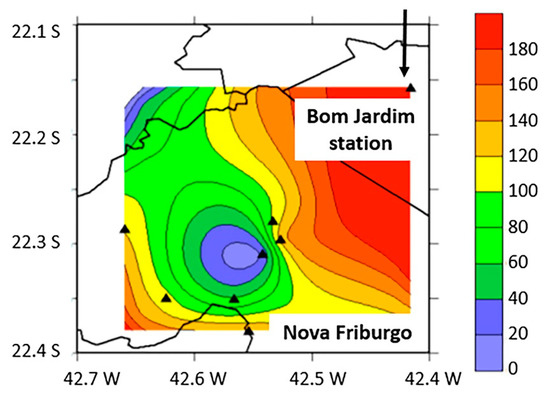
Figure 4. Interpolation of rainfall stations in the Rio Grande Basin for the rain observed on 11 January 2011 (mm/24 h). Source: Reprinted/adapted with permission from Ref. [24]. 2020. Barcellos and Cataldi.

The magnitude of the disaster took proportions beyond what has ever been seen in the country, not only by the impacts from flooding and inundation, but also by numerous mass movements triggered by heavy rains (Figure 5), affecting especially the municipalities of Nova Friburgo, Petrópolis and Teresópolis [3,21]. According to the report conducted by the World Bank, it is estimated that the cost of losses and damages to the public and private sectors totaled approximately $ 917 million [21].

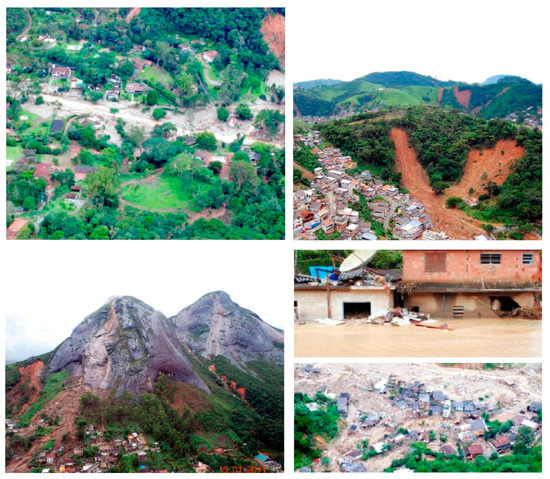
Figure 5. Photos from the 2011 disaster in the mountainous region of the Rio de Janeiro. Source: Reprinted/adapted with permission from Ref. [21]. 2012. Banco Mundial; Ref. [25]. 2011. DRM-RJ.

Historically, extreme events of hydrological origin occur frequently in the mountainous region of the Rio de Janeiro. The geomorphological aspects, such as steep slopes, high drainage, poorly developed soils, and the presence of fractures in the escapes, combined with the rainy season, favor the susceptibility to erosive and hydrological processes [3,26]. In addition, the occupation of irregular and risky areas makes these populations increasingly exposed to these events.

According to the report by the Ministry of the Environment, of the 657 landslides mapped in the municipality of Nova Friburgo, 90% occurred in areas with some anthropic intervention [27]. Actions, such as deforestation and the opening of roads and pastures, have influenced erosion processes and the destabilization of slopes in this area [27].

The disasters that occurred in the mountainous region of the state of Rio de Janeiro in 2011 show that prevention measures are essential to reduce the impacts. Real-time monitoring and prognosis of atmospheric events, river levels, and previous soil moisture conditions are essential measures to minimize the number of fatalities. Unfortunately, these actions have not been implemented, with no strengthening of civil defenses or the creation of situation rooms that could offer security to the population. Despite the progress in the legal framework and the development of new instruments to deal with natural disasters in the country, this became evident in other events that occurred in the same mountainous region, such as the one in Petrópolis in 2022, where again there was a large number of deaths.

2.3. SWAT Hydrological Model

The SWAT hydrological model is continuous in time, conceptual and based on physical processes that operate in daily time steps [12]. In this model, the watershed is divided into sub-basins consisting of a set of hydrologic response units (HRUs), defined by homogeneity in management, soil type, and land use and land cover, which contributes to improved representation of the study area and accuracy in the simulations [10].After the simulation in the land phase, the products such as flow, sediment, nutrients, pesticides and bacteria are routed in the main channel of each sub-basin and subsequently summed over the watershed [9]. All physical processes are governed by the watershed water balance summarized in Equation (1).

$$S{W}_t=S{W}_0+{\Sigma }_{i=1}^t\left(R_{day}-Qsurf-E_a-W_{seep}-Q_{gw}\right)$$

(1)

where $S{W}_t$ is the final amount of water in the soil (mm H₂O).$S{W}_0$ is initial soil water moisture on day i (mm H₂O). T is the time (days). $R_{day}$ is the precipitation (mm H₂O).$Qsurf$ is the runoff per unit area on day i (mm H₂O). $E_a$ is the evaporation on day i (mm H₂O). $W_{seep}$ is the water entering the wetland from the soil profile on day i (mm H₂O). $Q_{gw}$ is the return flow rate on day i (mm H₂O).

2.3.1. SWAT Input Data

SWAT’s main input data correspond to the digital elevation model (DEM), the land use and land cover map, the pedology map and its physical parameters, and the climatic data, summarized in rainfall, minimum and maximum temperature, solar radiation, relative humidity, and wind speed.

The DEM allows SWAT to calculate slope and generate the hydrographic network and subbasins. The study basin was delineated from the DEM (Figure 6a) of 30 m spatial resolution obtained from the Shuttle Radar Topographic Mission (SRTM) (https://earthexplorer.usgs.gov/ (accessed on 18 April 2018)) [28]. The use of this product for the Brazilian territory is satisfactory for a scale of between 1:50,000 and 1:100,000 [29]. Furthermore, this version of DEM SRTM showed better results when compared to ALOSWorld 3D and ASTER GDEM v.2 products [30].

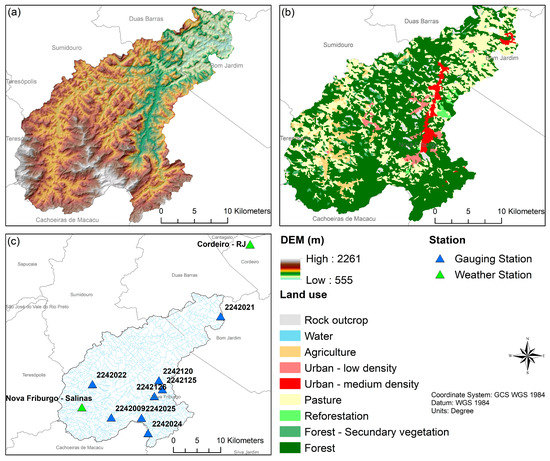
Figure 6. (a) Digital elevation model of the upper Rio Grande Basin. Source: Reprinted/adapted with permission from Ref. [28] 2013. NASA. (b) Land Use and Land Cover map of the Rio Grande Basin, RJ. Source: Reprinted/adapted with permission from Ref. [31] 2018. INEA. (c) Location of the pluviometric posts and climate stations of the upper Rio Grande Basin, RJ.

The land use and land cover map was obtained from the geospatial database of the State Environmental Institute (INEA) (https://inea.maps.arcgis.com/home/index.html (accessed on 25 April 2018)) [31]. The map of the year 2007 at the scale of 1:100,000 was used, since it characterized the landscape features prior to the event (Figure 6b).

For comparison purposes, the rainfall data were taken from the study [17], the authors selected the stations with coincident periods and that presented at least 5 years of data. These are available in the Hidroweb database (http://hidroweb.ana.gov.br (accessed on 3 May 2018)) of the National Water Agency (ANA) and in the flood alert system created by INEA (http://alertadecheias.inea.rj.gov.br (accessed on 3 May 2018)) (Figure 6c and Table 1).

Table 1. Rainfall Stations.

Code	Name	Responsible	Latitude	Longitude
2242126	Olaria	INEA	−22.3086°	−42.5422°
2242125	Ypu	INEA	−22.2956°	−42.5269°
2242120	Nova Friburgo	INEA	−22.2786°	−42.5336°
2242024	Teodoro de Oliveira	ANA	−22.3789°	−42.5542°
2242025	Castanhas do Conego	ANA	−22.3500°	−42.5542°
2242009	São Lourenço	ANA	−22.3494°	−42.6242°
2242022	Fazenda Mendes	ANA	−22.2858°	−42.6600°
2242021	Bom Jardim	ANA	−22.1567°	−42.4161°

Due to the need to heat the SWAT model, the time series of rainfall data used corresponded to the period 1 January 2008 to 15 January 2011, and the flow data from 1 January 2009 to 15 January 2011, acquired from the fluviometric station Bom Jardim (58827000), situated at the same location as the rainfall station (2242021). Through the stations operated by INMET (Figure 6c), the solar radiation and wind speed data were obtained through the Nova Friburgo-Salinas station, while the relative humidity and minimum and maximum temperature data were obtained through the Cordeiro-RJ station. In the cases of missing data, the global climate generator CFSR (Climate Forecast System Reanalysis), provided by the National Centers for Environmental Prediction (NCEP) (https://globalweather.tamu.edu/ (accessed on 5 May 2018)) was applied.

The pedological map of the basin corresponds to the soil map of the Geoenvironmental Study of the State of Rio de Janeiro, published in 2000, at the scale of 1:250,000 and executed by the Brazilian Agricultural Research Corporation (EMBRAPA) [32]. The soil classes adopted are based on the first level exposed in Table 2, while the physical parameters are obtained from the literature, and sources expressed in Table 3.

Table 2. Characteristics of soil classes in the Rio Grande Basin, RJ.

Soil Class	Features
Argissolos (Podzolic)	Deep soils with good drainage, not hydromorphic, and red and yellow textural B horizon.
Cambisols	Poorly developed, shallow, non-hydromorphic soils with considerable silt content.
Latosols	Well developed soils with a high degree of weathering, presenting great depth, good drainage and latossolic b horizon.
Litholic Soils	Soils with a low degree of development, presenting little depth with the A horizon over rock or in B or C horizons of little thickness. In its composition, gravel and rock pebbles predominate.

Source: Reprinted/adapted with permission from Ref. [32]. 2000. Filho, Lumbreras and dos Santos.

Table 3. Soil parameters and their sources.

Soil Parameters	Source
Albedo	[33]
Water capacity in the soil	[34,35]
Hydraulic conductivity	[36]
Apparent density	[37]
Erodibility Factor	[38]
Granulometry	[39]
Layer Depth	[39]
Soil texture	[40]

2.3.2. Calibration and Validation of SWAT

Calibration is the step of adjusting the model by varying its sensitive parameters in order to obtain the best relationship between a given time series of observed or estimated data and the data predicted in the modeling. SWAT has a range of parameters aimed at hydrological, sedimentological, nutrient and pesticide calibration. Because of the lack of other data, this simulation was limited to the hydrologic calibration by comparing the estimated flow data with those calculated by the model. Once the model is calibrated, the validation of the desired period is performed. The most sensitive calibration parameters and their modifications are observed, as shown in Table 4.

Table 4. Calibration Parameters Definition and their Modifications.

Parameter	Definition	Setting
		Add	Multiplication	Replacement
CANMN	Maximum water storage in the canopy (mm H2O)	5	-	-
CN	Curve number	-	0.6	-
GW_DELAY	Time interval for aquifer recharge (days)	-	-	500
SOL_K	Saturated hydraulic conductivity (mm/hour)	−3	-	-
SOL_K(Cambisols)	Saturated hydraulic conductivity (mm/hour) for the Cambisols	−10	-	-
RCHRG_DP	Water percolation fraction into the deep aquifer (mm)	0.3	-	-

Thus, the minimization of lateral runoff was sought through the SOL_K parameters, while, to increase water retention in the aquifer and the consequent elevation of the base flow, modifications were assigned to the GW_DELAY and CANMX values and, finally, to reduce the peaks, the CN and RCHRG_DP values were altered. It is noteworthy that in the SOL_K parameter, initially the value was changed for all soil classes, and later a new change occurred only for the areas that were Cambissolo type, because this presents the highest conductivity among the remaining soils.

The calibration occurred in the period from 1 January 2008 to 28 December 2010, in view of the heating of one year adopted in 2008. The flow data for the month of January 2011 used in the validation were results of constitutions through interpolations of neighboring posts made by ANA due to the lack of measurements in this period. Although the event occurred on the 11th and 12th, the flood wave, in this constitution, occurs on the 14th, so the series analysis was performed until the 15th. Therefore, the validation occurred in the period from 1 January 2011 to 15 January 2011.

The reliability of the simulation is defined by the efficiency coefficients and statistical relationships that compare the observed or estimated data to that obtained from the modeling. The mean relative error (MRE) provides a concise evaluation, as it defines the error percentage between the observed and predicted data. In this sense, this coefficient was used in the evaluation of the simulation accuracy, expressed in Equation (2). Where $Em$ is the observed event, $\overline{Es}$ is the average of observed events; $Es$ is the simulating event and $n$ is the number of events.

$$ERM=\frac{1}{N}{{\displaystyle \sum }}_{i=1}^n\left(\frac{\left|Es-Em\right|}{Em}\right)·100$$

(2)

2.4. SMAP Hydrological Model

The deterministic, conceptual and concentrated model, SMAP, was developed in 1981 and operates in daily time steps; however, monthly or hourly intervals are possible in other versions, whose calibration can be performed manually and automatically [16]. In the daily simulation version, water storage and flux represented by SMAP result from the moisture balance of the linear soil, aquifer and surface reservoirs, expressed in Equations (3)–(5).

$$R_{solo}\left(t\right)=R_{solo}\left(t-1\right)+P\left(t\right)-Es\left(t\right)-Er\left(t\right)-Rec\left(t\right)$$

(3)

$$R_{sub}\left(t\right)=R_{sub}\left(t-1\right)+Rec\left(t\right)-Eb\left(t\right)$$

(4)

$$R_{sup}\left(t\right)=R_{sup}\left(t-1\right)+Es\left(t\right)-Ed\left(t\right)$$

(5)

where $R_{solo}\left(t\right)$ is the accumulated water volume in the soil reservoir on day t (mm). $R_{sub}\left(t\right)$ is the volume of water accumulated in the underground reservoir on day t (mm). $R_{sup}\left(t\right)$ is the volume of water accumulated in the surface reservoir on day t (mm). $P\left(t\right)$ is the average precipitation in the basin on day t (mm). $Es\left(t\right)$ is the runoff in the river section on day t (mm). $Ed\left(t\right)$ is the runoff from the surface reservoir on day t (mm). $Er\left(t\right)$ is the potential evapotranspiration in the basin on day t (mm). $Rec\left(t\right)$ is the recharge transferred from the soil reservoir to the underground reservoir on day t (mm) and $Eb\left(t\right)$ is the baseflow on day t (mm).

3. Results

3.1. SWAT

The results of the SWAT model consisted of hydrological and sediment production simulations. The delineation of the basin was processed according to the topographic characteristics and had as exutory the Bom Jardim fluviometric post (58827000), resulting in the generation of 27 sub-basins constituted by multiple HRUs, totaling 346 units.

3.1.1. Calibration and Validation

According to the tool included in the model, SWAT Check, in the uncalibrated simulation, the basin showed low baseflow contribution and high lateral and surface runoff rates, reflecting in simulated flows lower than the estimated flow in the dry period and high flood peaks in the wet period, Figure 7.

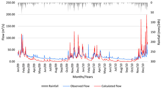
Figure 7. Uncalibrated comparison between estimated flow and simulated flow in SWAT defined by the left axis, while the right axis represents daily precipitation.

The adjustment of the calibration parameters was performed to meet the efficiency coefficient and approximate the behavior of the estimated flow series. The calibration reached an ERM of 18.46%, but the continuity of some peaks that could not be reduced is noted, as seen in Figure 8.

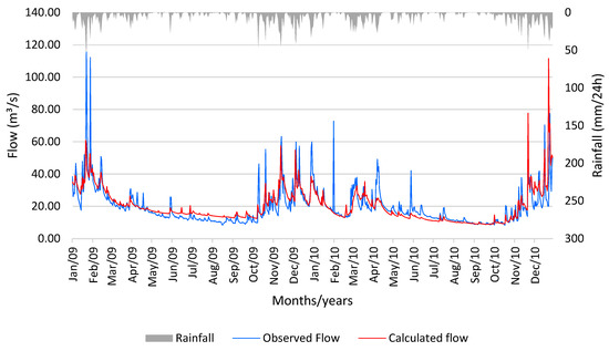
Figure 8. Calibrated comparison between estimated flow and simulated flow in SWAT defined by the left axis, while the right axis represents daily precipitation.

In the validation (Figure 9), the SWAT-simulated flows initially coincide with the ANA estimated flows, and on days 6 and 7 they underestimate them, but the model estimates a high peak on days 11 to 13, and they meet again on day 15. The average relative error resulted in a value of 88.73%.

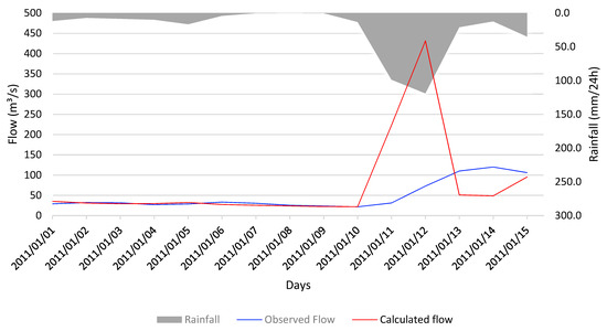
Figure 9. Comparison between estimated and simulated SWAT flow in the validation defined by the left axis, while the right axis represents daily precipitation.

The calibration performed in SWAT shows the tendency of the model to overestimate the peak flows, which may be an influential factor in the high values predicted in the event period.

However, despite the peak flood predicted by the model not being registered in the ANA data series, we cannot necessarily state that there was a failure of the simulation, since these flows were estimated and filled, because the measurement instruments and their respective stations were destroyed by the event. That is, the actual flow rate that occurred was probably much higher than the estimated one.

3.1.2. Sediment Production

Although sediment calibration was not performed due to lack of data, sediment production was analyzed with the purpose of identifying potential sedimentation areas, since the event was also characterized by landslides. Thus, the predicted production for day 12, the date of the occurrence of the highest flow calculated by the model, was estimated in the sub-basins and the sediment transport in the main channel (Table 5), which are represented, respectively, in Figure 10a,b.

Table 5. Sub-basin sediment production and transport in the main channel.

Sub-Basin	Sediment Produced (ton/ha)	Sediment Transported in the Channel (ton)	Soil Class *	Land Use *	Slope * (%)
1	1.410	2889	Podzolic	Pasture	39.6
2	0.001	18,630	Podzolic	Forest	26.6
3	1.190	1633	Cambisol	Forest	42.8
4	0.727	6530	Podzolic	Pasture	29.3
5	1.650	16,710	Podzolic	Pasture	38.6
6	2.050	2356	Podzolic	Pasture	40.2
7	0.020	28.60	Cambisol	Forest	38.6
8	1.310	12,000	Podzolic	Pasture	41.2
9	0.023	27.53	Rock outcrop	Forest	40.4
10	0.057	6939	Rock outcrop	Forest	36.9
11	0.177	7795	Cambisol	Forest	39.9
12	0.020	6469	Cambisol	Forest	35.6
13	0.176	1515	Latosol	Forest	35.8
14	0.056	134.90	Cambisol	Forest	34.2
15	6.380	6292	Cambisol	Forest	33
16	8.410	12,230	Cambisol	Forest	37.7
17	0.085	589.20	Latosol	Forest	35.2
18	1.670	2952	Cambisol	Forest	34
19	0.002	0.890	Latosol	Forest	38.3
20	9.470	18,010	Cambisol	Forest	36
21	0.002	0.596	Latosol	Forest	40.9
22	4.330	1162	Cambisol	Forest	39.5
23	2.290	201.10	Cambisol	Forest	36.2
24	1.250	2131	Cambisol	Forest	43.1
25	0.001	0.624	Cambisol	Forest	35.8
26	0.179	446	Rock outcrop	Forest	36.2
27	0.873	1343	Cambissolo	Forest	32.9

* Dominant characteristics of the sub-basin.

Figure 10. (a) Map of sediments produced in the sub-basins. (b) Map of sediments transported in the main channel. The limit of each sub-basin is referenced by the numbers indicated in the figure and can be associated with Table 5 and Table 6.

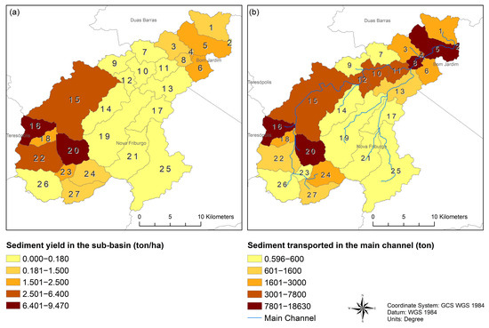
According to Figure 10a and Table 5, we can observe that sub-basins 15, 16, 20 and 22 were the most affected by erosive processes. The HRUs, which presented the highest values of sediment production, together with their respective sub-basins, are presented in Table 6, according to their physiographic characteristics—soil type, land use and slope class.

Table 6. Sediments produced at the HRU.

HRU	Sub-Basin	Sediment Produced (ton/ha)	Soil Class	Land Use	Slope Class
177	15	43.963	Cambisol	Agriculture	0–20
178	15	56.347	Cambisol	Agriculture	20–45
179	15	66.820	Latosol	Agriculture	20–45
180	15	31.722	Latosol	Agriculture	0–20
192	16	93.157	Cambisol	Agriculture	45–75
193	16	22.933	Cambisol	Agriculture	0–20
194	16	46.157	Cambisol	Agriculture	20–45
195	16	28.587	Latosol	Agriculture	0–20
196	16	57.844	Latosol	Agriculture	20–45
200	16	10.964	Cambisol	Pasture	75–100
259	20	34.032	Cambisol	Agriculture	0–20
260	20	51.082	Cambisol	Agriculture	20–45
264	20	13.378	Litholic	Pasture	45–75
291	22	46.813	Cambisol	Agriculture	20–45
292	22	23.345	Cambisol	Agriculture	0–20
293	22	20.408	Latosol	Agriculture	0–20
294	22	58.167	Latosol	Agriculture	20–45

Based on these data, it can be stated that the areas of agriculture, pasture, slope greater than 20% and soils of the type Cambisols and Latosols are the characteristics that prevail in areas of high sediment production. It can be seen that agriculture is the predominant factor in the areas with the highest production values, surpassing pasture, which, even in slope conditions greater than 75%, presented lower values. Furthermore, the highest production is associated with poorly developed soils (Cambisols) and high slope conditions, as seen in HRU 192.

When analyzing Figure 10b, the routing of sediments produced upstream elevates the sediment rates propagated in the downstream sub-basins. This situation applies to sub-basin 2, because, despite being classified as forest, the high values of sediments in the channel were enhanced by the propagation of the upstream sub-basins. Moreover, one should consider the erosion processes simulated in the channels, because they are also influencing factors, due to the erosive force of the current, which, in this event, was characterized by the flood wave.

3.2. SMAP

The study developed by [17] focused on hydrological modeling with the objective of researching the implementation of this model in the prediction of flows in the upper portion of the Rio Grande Basin upstream of Bom Jardim-RJ to aid disaster and urban flood management.

Calibration and Validation

The model calibration (Figure 11) was performed with data from the period November 2008 to December 2010, presenting an average relative error of 12%, whose underestimated flows occurred in the period December 2008 to February 2009, in contrast to the period of November and December 2009, in which flows were overestimated [17].

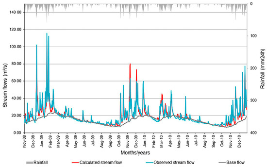
Figure 11. Calibrated comparison between estimated flow and simulated flow in SMAP defined by the left axis, while the right axis represents daily precipitation. Source: Reprinted/adapted with permission from Ref. [17]. 2020. Cavalcante, Barcelos and Cataldi.

The model validation (Figure 12) occurred in the period of December 29, 2010 to January 15, 2011, in order to evaluate the tool against the disaster prediction; the average relative error was 53%, whose results were underestimated throughout the series and overestimated during the event.

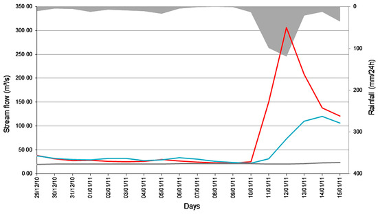
Figure 12. Validation of the SMAP model against the 2011 disaster from the comparison between estimated and simulated flow rates defined by the left axis, while the right axis represents daily precipitation. Source: Reprinted/adapted with permission from Ref. [17]. 2020. Cavalcante, Barcelos and Cataldi.

4. Discussion

According to the results, as we can see in Figure 9 and Figure 12, both models predicted the extreme flood event beginning on the 11th. The ERM of the model simulations (Table 7) infers that SMAP performed better in calibration and validation. The ERM of the latter stage is extremely important for evaluating the performance of the model in its predictions relative to the actual event and the reliability of the data generated. In this sense, comparing these two models, the SMAP presented, in this work, a better simulation performance, being more suitable for monitoring extreme flood events.

Table 7. ERM of SWAT and SMAP simulations.

ERM	SWAT	SMAP
Calibration	18.46%	12%
Validation	88.73%	53%

The high ERM generated by SWAT may be a reflection of the manual calibration performed or the need for a more extensive time series enabling a longer heating period, since the ideal is 2 to 3 years for hydrological modeling [41]. Moreover, the review conducted by [42] shows that SWAT’s flow forecasts have a good accuracy, especially when used at monthly scales, in contrast to the cases of extreme hydrological events. Furthermore, the low quality of the data prevented a satisfactory modeling and a more complete application of the model in this study.

SWAT is a complex model that simulates not only hydrological processes, but also processes of pollutant and sediment dispersion. Events such as the one that occurred in the mountainous region of Rio de Janeiro in 2011, characterized by floods and landslides, also reinforce its use as a warning tool for potential erosion areas, as exemplified in Figure 10, and for future studies related to the influence of land use and land cover on these erosive processes.

The integration of SWAT with the Geographic Information System (GIS) enables the visualization of data outputs facilitating the identification of impacted areas, and the ability to generate scenarios makes this model, when satisfactorily calibrated and validated, a powerful tool to assist not only in the monitoring of floods and landslides but also in decision making, problem solving, and prevention strategies.

5. Conclusions

The mountainous region of Rio de Janeiro is naturally susceptible to mass movements and floods in periods of heavy rainfall, due to its topographic variation, proximity to the sea and being an area of influence of the South Atlantic Convergence Zone—SACZ. Despite Law No. 12608/2012, which provided for the creation of prevention measures and environmental monitoring in order to increase resilience and reduce the number of people affected, these events are recurrent and have still caused fatalities in this region, as seen in Petrópolis in 2022, reinforcing the need for new actions for the minimization of vulnerability and risk.

In this sense, hydrological models, besides being an alternative for predicting these hydrological events, are also indispensable for territorial planning aimed at managing water resources and increasing the system’s resilience to disturbances and impacts.

The methodology consisted of comparing the SMAP model simulations performed by [17] to those generated in this work with the SWAT model in predicting the extreme flood event that occurred in the upper portion of the Rio Grande Basin in 2011, in order to test the viability and performance of these models as monitoring systems. The results predicted in the validation between SWAT and SMAP, allow us to affirm that both models calculated flows that underestimated and, in some moments, coincided with the ANA flows until day 11 of the time series, and overestimated the peak flow initiated on this day; however, they were able to predict the occurrence of an extraordinary flood, which for purposes of warning the population is a very important result.

The calibration performed in the SWAT model presented an average relative error of 18.46%, higher than that obtained by study [17] with the SMAP model, which corresponded to 12%, while in the validation, the error in the first model reached the value of 88.73% and in the second, 53%. Thus, according to these results, SMAP presented, in this work, a better performance in the simulation of the event in relation to SWAT.

The results obtained infer that SMAP is more suitable for monitoring due to its performance in the simulation, but also due to its simplicity of use and need for little data. Although the SWAT allows a more complete study of the hydrographic basin, and has other applications, the simulation in this event resulted in results very similar to those of the SMAP. Therefore, we can draw two great lessons from this study:

-

For basins with low hydrometeorological and geographic monitoring, the application of simpler models, such as SMAP, can generate results similar to those obtained with more complex models;

-

For the application of more complete hydrological models that better reproduce floods and flood waves, it is necessary to expand the monitoring network. Without this expansion, the results will always be limited to simplistic simulations and not very detailed, which can help in the prevention of disasters, but with a high degree of uncertainty.

The event in the mountainous region of Rio de Janeiro, in 2011, promoted new advances in the country in coping with natural disasters, but they are still events that cause damage and victims wherever they occur. Hydrological models prove to be fundamental in predicting these phenomena and in guiding the strategies to be adopted. The anticipation of knowledge of the event is a critical importance for the government, together with the civil defense, to take the necessary prevention and mitigation measures, which can save countless lives.

References

- World Bank; United Nations. Natural Hazards, Unnatural Disasters: The Economics of Effective Prevention; The World Bank: Washington, DC, USA, 2010; ISBN 978-0-8213-8050-5. [Google Scholar]
- Centre for Research on the Epidemiology (CRED). 2021 Disasters in Numbers; CRED: Brussels, Belgium, 2022; p. 8. Available online: https://cred.be/sites/default/files/2021_EMDAT_report.pdf (accessed on 10 October 2022).
- Centro Universitário de Estudos e Pesquisas Sobre Desastres da Universidade Federal de Santa Catarina (CEPED-UFSC). Atlas Brasileiro de Desastres Naturais: 1991 a 2012, 2nd ed.; UFSC: Florianópolis, Brasil, 2013; p. 126. [Google Scholar]
- BRASIL. LEI n°. 12.608, de 10 de Abril de 2012. Institui a Política Nacional de Proteção de Defesa Civil. Casa Civil. Subchefia para Assuntos Jurídicos. 2012. Available online: https://www.planalto.gov.br/ccivil_03/_ato2011-2014/2012/lei/l12608.htm (accessed on 15 January 2018).
- Marcelino, E.V. Desastres Naturais e Geotecnologias: Conceitos Básicos; CRS/INPE, Santa Maria: Singapore, 2008; p. 38. [Google Scholar]
- Sausen, T.M.; Lacruz, M.S.P. Sensoriamento Remoto para Desastres; Oficina de Textos: São Paulo, Brazil, 2015; p. 288. ISBN 978-85-7975-175-2. [Google Scholar]
- Tucci, C.E.M. Hidrologia: Ciência e Aplicação, 2nd ed.; Universidade/UFRGS: Porto Alegre, Brazil, 2001. [Google Scholar]
- Tucci, C.E.M. Modelos Hidrológicos; Universidade/UFRGS: ABRH—Associação Brasileira de Recursos Hídricos: Porto Alegre, Brazil, 1998; p. 668. [Google Scholar]
- Neitsch, S.L.; Arnold, J.G.; Kiniry, J.R.; Williams, J.R. Soil and Water Assessment Tool Theoretical Documentation: Version 2009; Agricultural Research Service, Grassland, Soil and Water Research Laboratory, Blackland Research and Extension Center, Texas AgriLife Research, Water Resources: College Station, TA, USA, 2011; p. 618. Available online: http://swatmodel.tamu.edu/documentation/ (accessed on 10 January 2018).
- Arnold, J.G.; Kiniry, J.R.; Srinivasan, R.; Williams, J.R.; Haney, E.B.; Neitsch, S.L. Input/output Documentation Version 2012. Texas Water Resources Institute TR-439. 2012. Available online: http://swat.tamu.edu/documentation/2012-io/ (accessed on 1 February 2018).
- Arnold, J.G.; Moriasi, D.N.; Gassman, P.W.; Abbaspour, K.C.; White, M.J.; Srinivasan, R. SWAT: Model use, calibration, and validation. Trans. ASABE 2012, 55, 1491–1508. [Google Scholar] [CrossRef]
- Arnold, J.G.; Srinivasan, R.; Muttiah, R.S.; Williams, J.R. Large area hydrologic modeling and assessment. Part I. Model development. J. Am. Water Resour. Assoc. 1998, 34, 73–89. [Google Scholar] [CrossRef]
- Dile, Y.T.; Daggupati, P.; George, C.; Srinivasan, R.; Arnold, J. Introducing a new open source GIS user interface for the SWAT model. Environ. Model. Softw. 2016, 85, 129–138. [Google Scholar] [CrossRef]
- Gassman, P.W.; Reyes, M.R.; Green, C.H.; Arnold, J.G. The Soil and Water Assessment Tool: Historical development, applications, and future research directions. Trans. ASABE 2007, 50, 1211–1250. [Google Scholar] [CrossRef]
- Bou, A.S.F.; de SÁ, R.V.; Cataldi, M. Flood forecasting in the upper Uruguay River basin. Nat. Hazards 2015, 79, 1239–1256. [Google Scholar]
- Lopes, J.E.G.; Braga, B.P.F., Jr.; Conejo, J.G.L. SMAP—A Simplified Hydrological Model. Applied Modelling in Catchment Hydrology; Singh, V.P., Ed.; Water Resources Publications: Lone Tree, CO, USA, 1982; pp. 167–176. [Google Scholar]
- Cavalcante, M.R.G.; Barcelos, P.C.L.; Cataldi, M. Flash flood in the mountainous region of Rio de Janeiro state (Brazil) in 2011: Part I—Calibration watershed through hydrological SMAP model. Nat. Hazards 2020, 102, 1117–1134. [Google Scholar] [CrossRef]
- Dantas, M.E.; Shinzato, E.; Medina, A.I.M.; Silva, C.R.; Pimentel, J.; Lumbreras, J.F.; Calderano, S.B. Diagnóstico Geoambiental do Estado do Rio De Janeiro; CPRM: Brasília, Brazil, 2000. Available online: http://rigeo.cprm.gov.br/jspui/bitstream/doc/17229/14/rel_proj_rj_geoambiental.pdf (accessed on 16 March 2018).
- Bernardes, L.N.C. Tipos de clima do estado do Rio de Janeiro. Rev. Bras. De Geogr. 1952, 14, 57–80. [Google Scholar]
- Velloso, H.P.; Filho, A.L.R.R.; Lima, J.C.A. Classificação da Vegetação Brasileira Adaptada a um Sistema Universal; IBGE: Rio de Janeiro, Brazil, 1991; 124p. [Google Scholar]
- Banco Mundial. Avaliação de Perdas e Danos: Inundações e Deslizamentos na Região Serrana do Rio de Janeiro-Janeiro de 2011. Relatório elaborado pelo Banco Mundial com apoio do Governo do Estado do Rio de Janeiro. 2012; p. 63. Available online: https://documents1.worldbank.org/curated/pt/260891468222895493/pdf/NonAsciiFileName0.pdf (accessed on 8 February 2018).
- Dourado, F.; Arraes, T.C.; Silva, M.F. O Megadesastre da Região Serrana do Rio de Janeiro—As Causas do Evento, os Mecanismos dos Movimentos de Massa e a Distribuição Espacial dos Investimentos de Reconstrução no Pós-Desastre; Anuário do Instituto de Geociências—UFRJ: Rio de Janeiro, Brazil, 2012; Volume 35, pp. 43–54. [Google Scholar]
- Freitas, C.M.; Carvalho, M.L.; Ximenes, E.F.; Arraes, E.F.; Gomes, J.O. Vulnerabilidade socioambiental, redução de riscos de desastres e construção da resiliência: Lições do terremoto no Haiti e das chuvas fortes na Região Serrana, Brasil. Ciência Saúde Coletiva 2012, 17, 1577–1586. [Google Scholar] [CrossRef] [PubMed]
- Barcellos, P.C.L.; Cataldi, M. Flash Flood and Extreme Rainfall Forecast through One-Way Coupling of WRF-SMAP Models: Natural Hazards in Rio de Janeiro State. Atmosphere 2020, 102, 834. [Google Scholar] [CrossRef]
- Departamento de Recursos Minerais (DRM-RJ). Megadesastre da Serra Jan 2011. Available online: http://www.drm.rj.gov.br/index.php/downloads/category/13-regioserrana?download=48%3Amegadesastre-da-serra-jan-2011-pdf (accessed on 10 October 2022).
- Carvalho, R.C.; Francisco, C.N.; Salgado, C.M. Condicionantes geomorfológicos e da cobertura da terra na ocorrência de movimentos de massa na região serrana do Rio de Janeiro. Cad. De Geogr. 2019, 29, 27–44. [Google Scholar]
- BRASIL. Ministério do Meio Ambiente. Secretaria de Biodiversidade de Florestas. Relatório de Inspeção. Área atingida pela tragédia das Chuvas da Região Serrana do Rio de Janeiro. Brasília, Distrito Federal. 2011. Available online: https://fld.com.br/wp-content/uploads/2019/07/relatoriotragediarj_182.pdf (accessed on 10 October 2022).
- Nasa, J.P.L. NASA Shuttle Radar Topography Mission Global 1 arc second. NASA EOSDIS Land Processes DAAC. 2013. Available online: https://doi.org/10.5067/MEaSUREs/SRTM/SRTMGL1.003 (accessed on 18 April 2018).
- Barros, R.S.; Cruz, C.B.M. Avaliação da altimetria do modelo digital de elevação SRTM. In Proceedings of the Anais XIII Simpósio de Sensoriamento Remoto, Florianópolis, Brasil, 21–26 April 2007; pp. 1243–1250. Available online: http://marte.sid.inpe.br/col/dpi.inpe.br/sbsr@80/2006/11.15.13.17/doc/1243-1250.pdf (accessed on 12 April 2018).
- Viel, J.A.; Rosa, K.K.; Junior, C.W.M. Avalição da Acurácia Vertical dos Modelos Digitais de Elevação SRTM, ALOS World 3D e ASTER GDEM: Um estudo de Caso no vale Vinhedos, RS-Brasil. Rev. Bras. Geogr. Física 2020, 13, pp. 2255–2268. [Google Scholar] [CrossRef]
- Instituto Estadual do Ambiente (INEA). Base de Dados Geoespaciais. Uso do Solo e Cobertura Vegetal. Metadados e Download de Camadas: Monitoramento do Uso do Solo. Available online: https://inea.maps.arcgis.com/apps/MapSeries/index.html?appid=00cc256c620a4393b3d04d2c34acd9ed (accessed on 25 April 2018).
- Filho, A.C.; Lumbreras, J.F.; dos Santos, R.D. Estudo Geoambiental do Estado do Rio de Janeiro—Os solos do Estado do Rio de Janeiro; CPRM—Serviço Geológico do Bras: Brasília, Brazil, 2000. [Google Scholar]
- Thompson, D.; Barbosa, I.; Oliveira, R.A.A.C. Avaliação da variação do albedo de superfície tipológicas de uso e cobertura terrestre. Rev. Bras. Cart. 2017, 69, 375–387. [Google Scholar]
- Salter, P.J.; Williams, J.B. The influence of texture on the moisture characteristics of soils. IV. A method of estimating the available water capacities of profiles in the field. J. Soil Sci. 1967, 18, 174–181. [Google Scholar] [CrossRef]
- Salter, P.J.; Williams, J.B. The influence of texture on the moisture characteristics of soils. V. Relationships between particle size composition and moisture contents at the upper and lower limits of available water. J. Soil Sci. 1969, 20, 126–131. [Google Scholar] [CrossRef]
- Dent, D.; Yong, A. Soil Survey and Land Evaluation; Allen e Unwin: London, UK, 1981; p. 278. [Google Scholar]
- Taylor, H.M.; Roberson, G.M.; Parker, J.J., Jr. Soil strength-root penetration relations to medium to coarse-textured soil materials. J. Soil Sci. 1966, 102, 18–22. [Google Scholar] [CrossRef]
- Williams, J.R. The EPIC Model. In Computer Models of Watershed Hydrology, Chapter 25; Singh, V.P., Ed.; Water Resources Publications: Lone Tree, CO, USA, 1995. [Google Scholar]
- Empresa Brasileira de Pesquisa Agropecuária (Embrapa). Sistema de Informações de Solos Brasileiros. 2018. Available online: https://www.sisolos.cnptia.embrapa.br/ (accessed on 18 April 2018).
- Soil Science Division Staff. Soil Survey Manual; Ditzler, C., Scheffe, K., Monger, H.C., Eds.; USDA Handbook 18; Government Printing Office: Washington, DC, USA, 2017. [Google Scholar]
- Daggupati, P.; Pai, N.; Ale, S.; Douglas-Mankin, K.R.; Zeckoski, R.W.; Jeong, J.; Parajuli, P.B.; Saraswat, D.; Youssef, M.A. Recommended calibration and validation strategy for hydrologic and water quality models. Trans. ASABE 2015, 58, 1705–1719. [Google Scholar]
- Borah, D.K.; Bera, M. Watershed-scale hydrologic and nonpoint-source pollution models: Review of applications. Trans. ASAE 2004, 47, 789–803. [Google Scholar] [CrossRef]
Disclaimer/Publisher’s Note: The statements, opinions and data contained in all publications are solely those of the individual author(s) and contributor(s) and not of MDPI and/or the editor(s). MDPI and/or the editor(s) disclaim responsibility for any injury to people or property resulting from any ideas, methods, instructions or products referred to in the content. |
© 2023 by the authors. Licensee MDPI, Basel, Switzerland. This article is an open access article distributed under the terms and conditions of the Creative Commons Attribution (CC BY) license (https://creativecommons.org/licenses/by/4.0/).