Autumn Surface Wind Trends over California during 1979–2020

Abstract

Surface winds over California can compound fire risk during autumn, yet their long-term trends in the face of decadal warming are less clear compared to other climate variables like temperature, drought, and snowmelt. To determine where and how surface winds are changing most, this article uses multiple reanalyses and Remote Automated Weather Stations (RAWS) to calculate autumn 10 m wind speed trends during 1979–2020. Reanalysis trends show statistically significant increases in autumn night-time easterlies on the western slopes of the Sierra Nevada. Although downslope windstorms are frequent to this region, trends instead appear to result from elevated gradients in warming between California and the interior continent. The result is a sharper horizontal temperature gradient over the Sierra crest and adjacent free atmosphere above the foothills, strengthening the climatological nocturnal katabatic wind. While RAWS records show broad agreement, their trend is likely influenced by year-to-year changes in the number of observations.

1. Introduction

Surface winds modulate fire weather conditions over California in a myriad of ways, yet compared to other climate trends like multi-year drought [1], earlier spring snow melt [2], and a later onset of autumn precipitation [3,4,5], their long-term trends in the face of decadal warming are generally less clear. Although partially due to the sparse and relatively short nature of long-term wind data, the various wind patterns that can influence fire weather conditions also makes synthesizing their trends a daunting task.

Downslope windstorms are one such pattern that are ubiquitous during autumn across California. Over northern California and the Sierra Nevada, these windstorms are known as Diablo winds (previously Mono winds) [6,7], whereas over coastal southern California, they are called Santa Ana winds [8,9,10]. Dry, gusty Sundowners driven by the California coastal jet also enhance fire risk on the southern slopes of the Santa Ynez mountains [11,12,13,14]. These windstorms have each been responsible for the most destructive wildfires in their respective regions, including the Tubbs Fire (2017) [15,16], the Thomas Fire (2017) [17,18], and the Camp Fire (2018) [19,20,21].

Local-scale thermal gradients also generate a myriad of wind patterns, particularly over the Sierra Nevada. The daytime Washoe Zephyr, for example, blows over northeastern California during warm seasons in response to asymmetric heating between the Nevada desert and the western Sierra Nevada, posing unique challenges to fire containment operations and the spread of wildfire smoke [22,23]. Day-time and night-time anabatic and katabatic winds develop under quiescent conditions in response to asymmetric surface heating and cooling of terrain relative to the adjacent free troposphere; these temperature gradients lead to diurnal mountain slope, mountain–valley, and mountain–plain circulations on increasingly larger spatial scales [24]. The confluence of these winds and the resulting shears and turbulence have the potential to create challenging fire fighting conditions and take fire crews by surprise [23,25,26]. Furthermore, the katabatic mechanism, when considered between the relatively warm south Californian coast and cold high desert constitutes a type of Santa Ana wind, which, in the absence of onshore flow, is the primary control of Santa Ana variability [27]. Considering both thermally driven winds and synoptically driven windstorms is therefore important to build a broad picture of the evolving wind landscape over increasingly warmer decades, especially during the driest season in autumn.

Previous studies of wind trend in California are few and concern either future wind energy viability [28], coastal winds promoting upwelling [29], or are nationwide in scope [30,31]. From the perspective of fire weather, previous studies have understandably focused on downslope wind conditions, finding little or no discernible trend in the frequency or intensity of Diablo [32,33] or Santa Ana winds [34,35]. To the best of the authors’ knowledge, no studies exist on the long-term variability of Sundowners. Trends in these high-wind events often necessitates filtering climate data according to criteria of wind speed thresholds, attendant low humidities, and event duration, with trends then computed in event frequencies and wind speeds. Alternatively, a broader perspective may be achieved by computing trends in wind speed alone. Such an approach would reveal the wind circulations changing fastest, and may indicate not just changes in winds relevant for fire weather, but in those with other socioeconomic impacts, such as wind energy. To the best of our knowledge, no such study of historic surface wind speed trends exists for California.

This article therefore investigates regional trends in gridded 10 m wind speeds over California for autumns during 1979–2020, the season when fuels are generally drier and changes in the diurnal cycles of winds and the frequency and intensity of windstorms may significantly increase fire risk. Given the sparse and short record of weather station observations, wind speed trends are calculated from daily maximum winds in three reanalyses: the European Centre for Medium-Range Weather Forecasts ERA5 reanalysis, the NCEP North American Regional Reanalysis (NARR), and the National Centers for Environmental Prediction/National Center for Atmospheric Research (NCEP/NCAR) Reanalysis 1. Additionally, reanalysis trends are compared against a 30-year record of Remote Automated Weather Station (RAWS) observations spanning 1990–2020. Where trends are prominent and significant, we also seek to describe the underlying physical mechanism to elicit a deeper understanding of the state’s evolving wind landscape.

2. Datasets and Trend Method

Given the sparsity of weather station observations and their tendency to often extend no more than a decade, reanalyses are the next best datasets to investigate trends in surface wind speeds. This suitability is largely due to their consistent use of a single numerical weather prediction model and data assimilation scheme, as well as their wide catalog of meteorological variables that permit an examination of the potential physical mechanisms driving trends.

In this study, we use three reanalyses to investigate trends in 10 m winds: the European Centre for Medium-Range Weather Forecasts (ECMWF) ERA5 reanalysis [36], the North America Regional Reanalysis (NARR) [37], and the National Centers for Environmental Prediction/National Center for Atmospheric Research (NCEP/NCAR) Reanalysis 1 [38]. ERA5 has a 31 km horizontal grid spacing, 25 hPa vertical grid spacing in the lower troposphere, and is the first reanalysis with hourly output, allowing insight into diurnal variability. ERA5 can also correlate well with near-surface station winds over mountain terrain and most closely resembles the observed interannual variability compared to four other reanalyses [39,40]. Additionally, Molina et al. [41] compared ERA5 10 m winds with 245 stations across Europe and determined that ERA5 is able to represent the diurnal variability of winds in light-to-strong conditions. NARR has a similar grid spacing to ERA5 (32 km), 3-hourly output capturing diurnal variability, and has been reported to have a small bias (less than 1 m s${}^{-1}$) for summertime and wintertime surface winds over the contiguous United States (CONUS) [37]. NARR also assimilates 10 m wind speeds from around 450 surface stations over the CONUS. Although the NCEP 1 reanalysis has coarse spatial (209 km) and temporal (6-hourly frequency) resolutions, it is used here as an additional dataset to compare 10 m trends with the modern reanalyses on larger scales.

One should also be aware that 10 m winds in reanalysis are not observations, but diagnostics from the model’s planetary boundary layer scheme. ERA5 10 m winds are calculated by extracting the wind speed at a blending height of 40 m and then extrapolating to 10 m using Monin–Obukhov theory and assuming a surface roughness length of 0.03 m, the roughness length of short grass surface. Zonal and meridional wind components are then calculated with this wind speed and the wind direction on the lowest model level (https://confluence.ecmwf.int/display/FUG/Section+9.3+Surface+Wind, accessed on 28 September 2023). NARR’s 10 m winds are likewise extrapolated from the wind at the model level nearest the ground minus a similarity function from Monin–Obukhov theory (Eqn. 4.6, [42]), but whose surface roughness varies with orography [30]. Another important difference between ERA5 and NARR is that NARR assimilates wind speeds from 450 land stations over the contiguous U.S. [37], although how many of these stations are in California is unknown to the authors. NCEP/NCAR 1 initially assimilated ocean surface wind speeds from microwave imaging; however, the process incurred logical and other issues and so were not incorporated in the final product [38]. As for ERA5 and NARR though, NCEP/NCAR 1 10 m winds are extrapolated from the lowest model level winds using Monin–Obukhov theory with a surface roughness derived from climatology [30]. Given the universal extrapolation approach to obtain surface winds and to evaluate our confidence in them, we also verified wind trends at other near-surface heights where permissible. This was only possible in ERA5 at 100 m where winds are interpolated from the nearest bounding model levels [43].

Trends from these data are calculated as follows. At each grid point, zonal and meridional wind components are used to calculate 10 m wind speeds at hourly (ERA5), 3-hourly (NARR) and 6-hourly (NCEP/NCAR) frequencies. For NARR, its zonal and meridional wind components are first treated with a Gaussian spatial filter to reduce noise that results from regridding its native grid to the Northern Lambert Conformal grid on which the data are archived. Filtering with a Gaussian kernel of degree $N=6$ (i.e., standard deviation $N/2\pi$) reduces 95% of noise on the order of 64 km, which is twice the NARR grid spacing. Next, daily maximum wind speeds in each dataset are identified and September–October–November (SON) seasonal averages computed from 1979 to 2020. Linear trends in these time series are computed as Theil–Sen estimators, whose statistical significance is determined with the Yue and Wang Modified Mann–Kendall test [44] to account for the temporal autocorrelation of winds, which can occur on 30-year timescales [31,45]. While this modified method has little effect on the magnitude of trends, it does increase the number of grid points with statistically significant trends (defined as those exceeding the 95% significance level) compared to standard Mann–Kendall testing.

From zonal and meridional wind components, we also calculate trends in maximum northerly, southerly, westerly, and easterly 10 m wind components during the day (0600–1700 PST) and at night (1800–0500 PST) to capture any diurnal changes in anabatic (upslope) vs. katabatic (downslope) winds. These 12 h periods contain 12, 4, and 2 reanalysis times in ERA5, NARR, and NCEP/NCAR reanalyses, respectively. Trends in seasonal averages of these daytime and night-time wind maxima are likewise evaluated with the Yue and Wang Modified Mann–Kendall test.

Further to reanalysis trends, we examine trends in daily maximum wind speeds from 28 Remote Automated Weather Stations (RAWS) archived at the Western Regional Climate Center of the Desert Research Institute (DRI) (https://raws.dri.edu/, accessed on 27 September 2023). While this network incorporates far more than 28 stations, the stations chosen are those with a 30-year record spanning 1990–2020. As these stations are in remote areas, often over complex terrain, and they provide a crucial dataset for comparing reanalysis trends as well as offering long-term trends in areas where reanalysis typically underestimate winds. Trends at these locations are also calculated from seasonal averages of daily maximum winds using Yue and Wang Modified Mann–Kendall testing.

Where trends are significant and prominent, we investigate potential regional vs. local-scale processes. Specifically, regional processes include MSLP gradients and downslope windstorms, with the latter identified from the gridded ERA5-derived dataset of Abatzoglou et al. [46]. This dataset contains two variables: the gridded daily occurrence of a downslope windstorm, indicated by 1 (present) or 0 (absent), and the associated wind direction. While not matching our period of study exactly, this period is still sufficiently long to elicit the influence of windstorms on any identified wind trends. On the other hand, we consider local-scale processes to be on the order of what reanalysis can resolve (i.e., approximately 30 km or greater). The Abatzoglou et al. [46] dataset has this resolution and can capture downslope windstorms, including California’s Sierra Nevada, suggesting that 30 km reanalyses offer some utility for examining surface winds over complex terrain. However, it is important to remember that these windstorms are often driven by larger-scale MSLP gradients, not local-scale processes. Therefore, surface winds and their underlying processes that occur on local scales should be thought of as in a gray zone of resolvability. Consequently, while surface winds can affect fire risk over complex terrain in terms of fire spread, this level of detail cannot be investigated here. Rather, we use the reanalyses as a first approach to assess long-term trends, which can serve as a reference and jumping-off point for future research.

3. Results

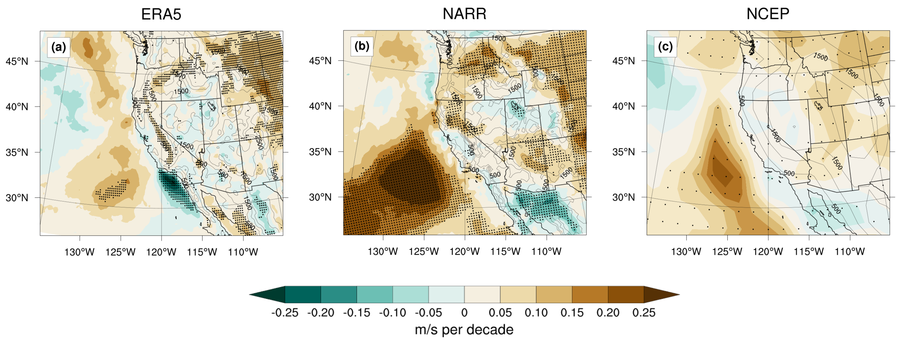
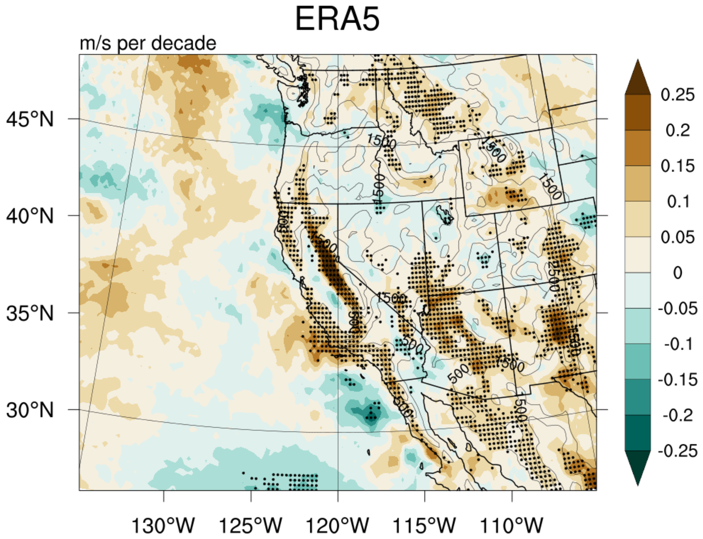
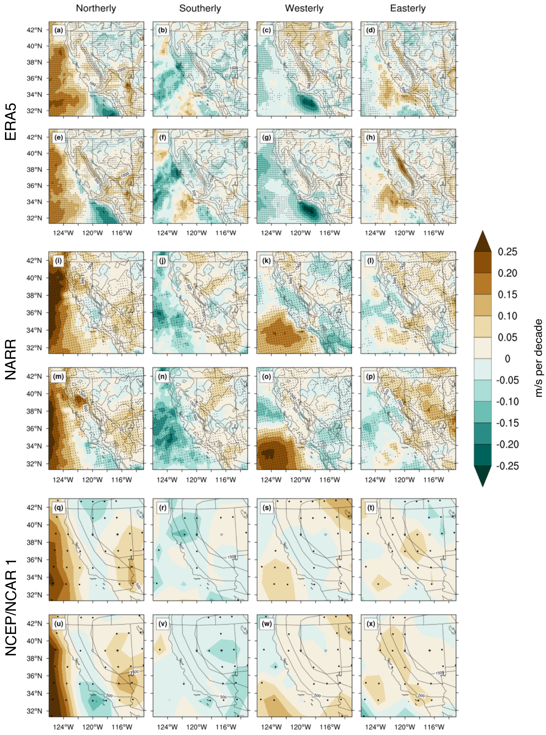
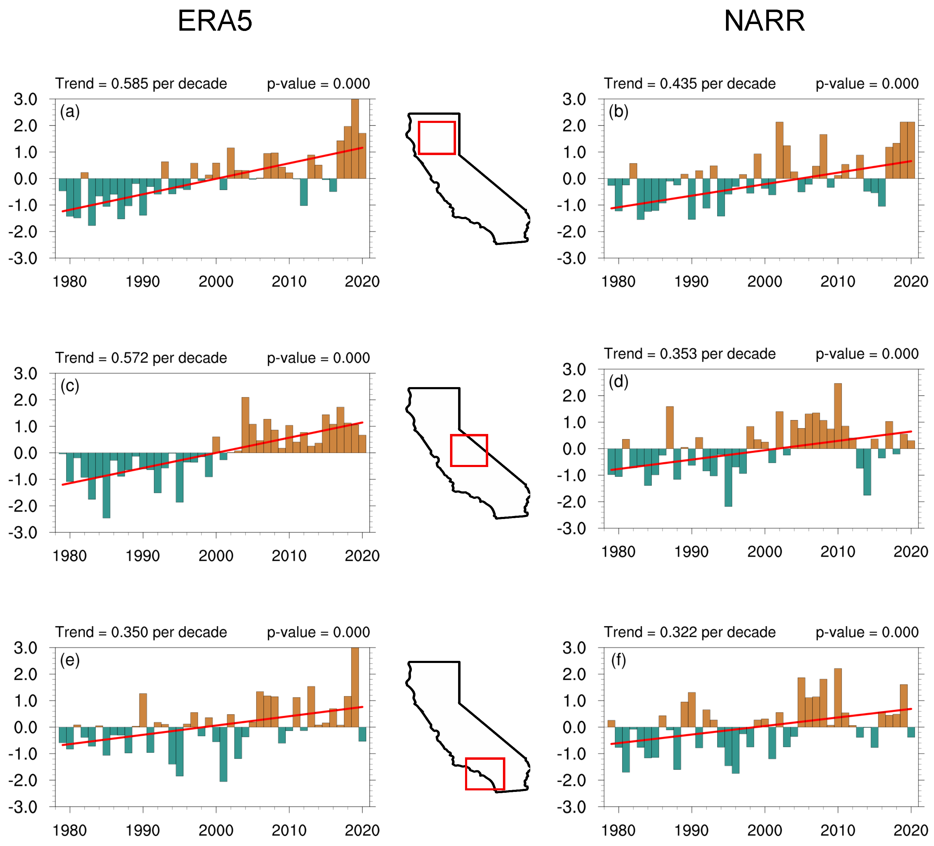
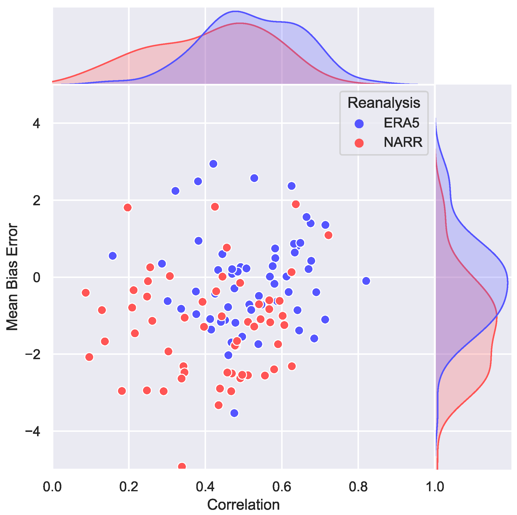
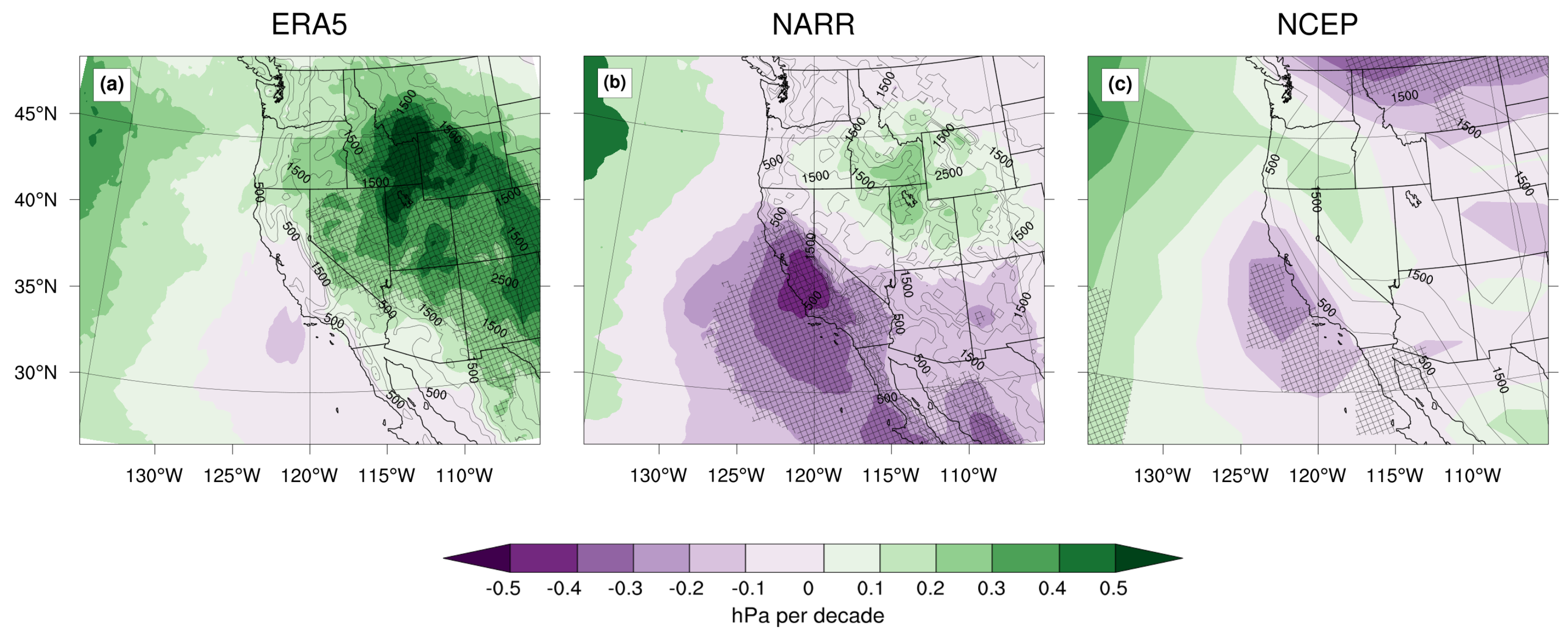
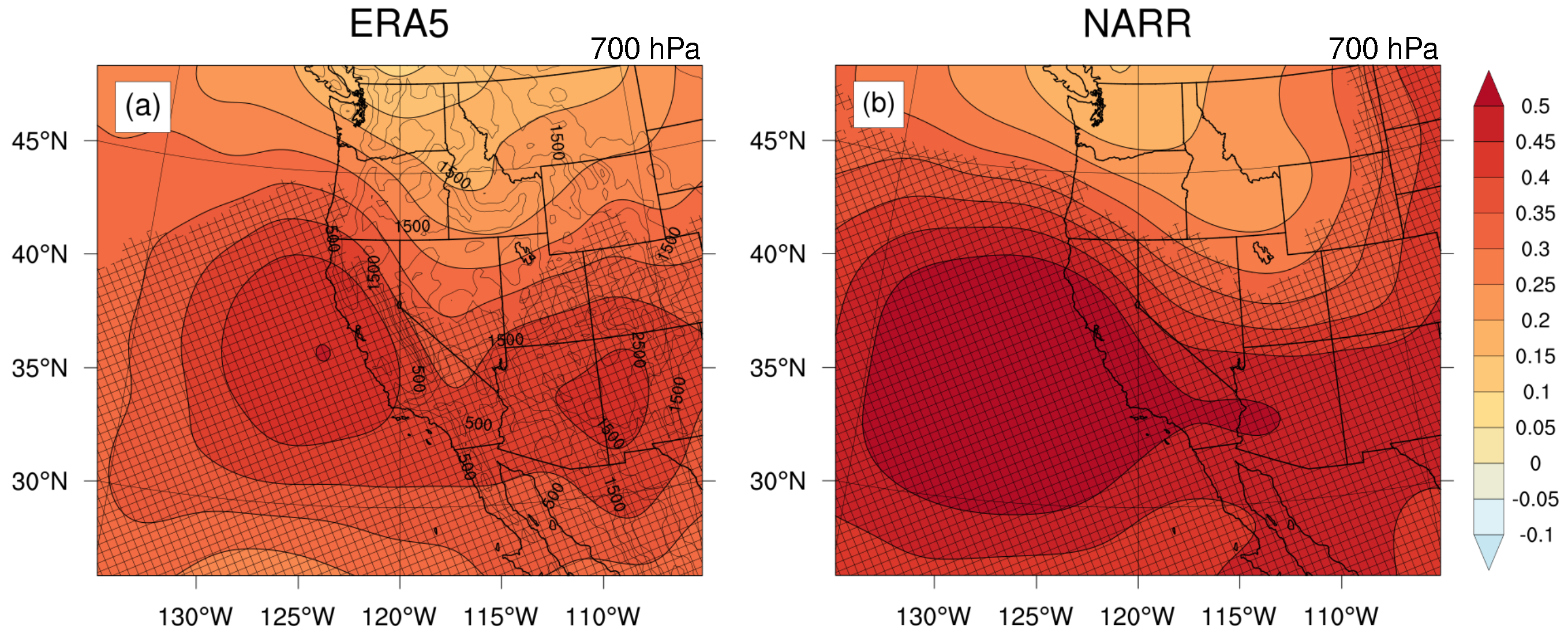
3.1. Reanalysis Trends

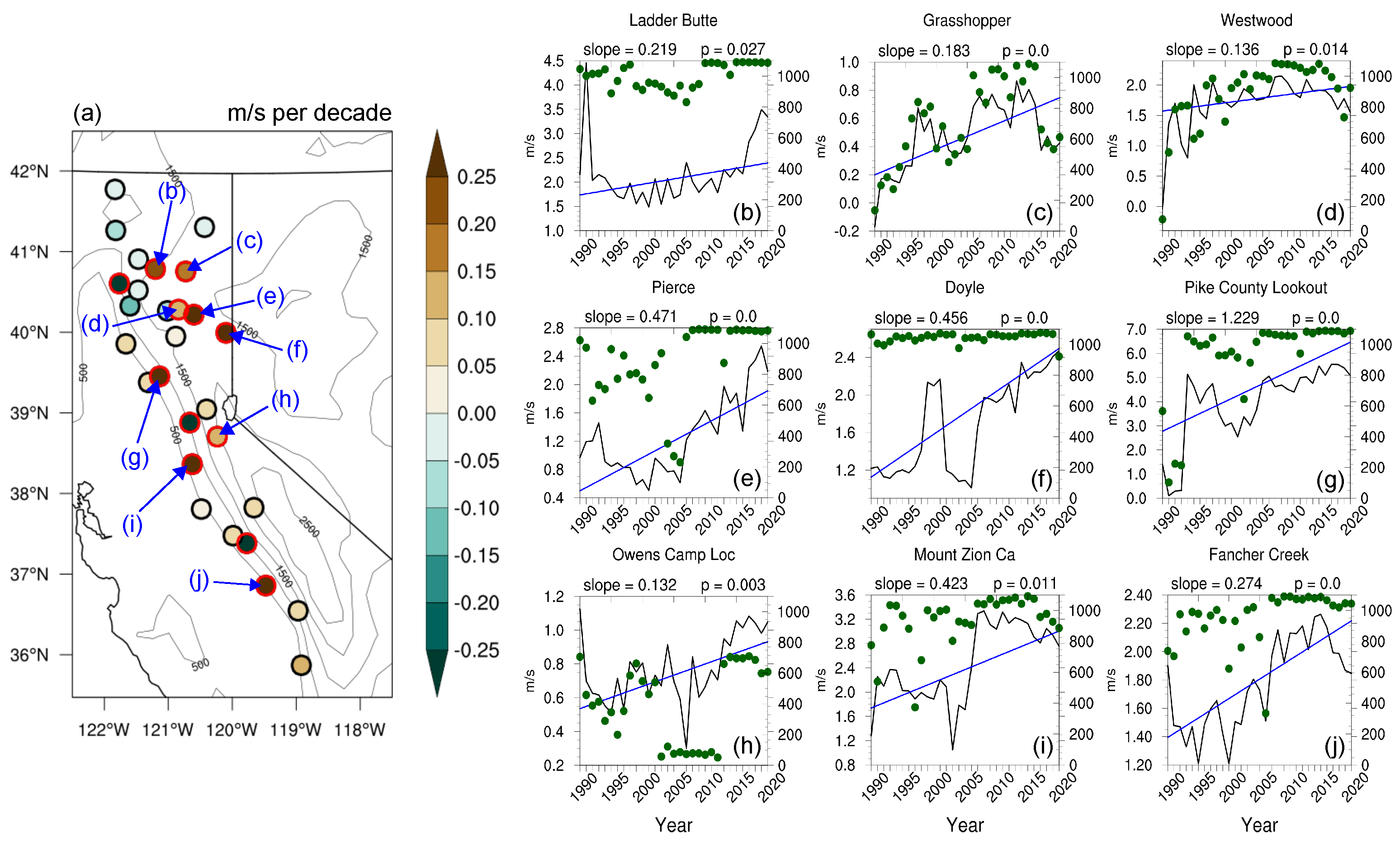
During SON, surface wind speeds over California are increasing most significantly over the Sierra Nevada (Figure 1). In ERA5, increases in daily maximum wind speeds span the entire western slopes of the mountain range, in addition to the Mendocino Range in the northwest of the state (Figure 1a). In NARR, increasing wind speeds are more confined to the northern Sierra Nevada and the Sacramento Valley (Figure 1b). As expected, these local trends are not found in the NCEP/NCAR reanalysis due to its coarser grid (Figure 1c). Furthermore, ERA5 also displays nearly identical significant and stronger trends in daily maximum wind speeds at 100 m (Figure 2), although trends at this height were not available in NARR or NCEP reanalyses. That this trend is seen at 100 m (where winds are interpolated between bounding model levels rather than extrapolated to the surface) indicates that wind trends do not result from assumptions in the surface extrapolation.

On the regional scale, trends show good cross-reanalysis agreement. ERA5 and NARR shows statistically increasing wind speeds off the California coast, consistent with ERA-Interim [47], and additionally in a broken, but broad, arc stretching from northern California, parts of the northern Intermountain West, and into the western Midwestern states. The NCEP/NCAR reanalysis also shows increasing wind speeds over the northern Intermountain West, but where it highlights strengthening winds between the Great Basin and Rocky Mountains, ERA5 and NARR show decreasing wind speeds. One other noticeable source of disagreement is in decreasing wind speeds over the Southern California Bight in ERA5 that is not present in either NARR or NCEP, despite the former’s similar grid spacing. Overall, however, reanalyses exhibit broad agreement in daily maximum wind trends over the western U.S.

Figure 3 shows the breakdown of trends by westerly, easterly, northerly, and southerly components. Strengthening winds over the Sierra Nevada in ERA5 are most closely associated with stronger night-time easterlies (cf. Figure 1a and Figure 3h) during both autumn and summer. NARR likewise highlights stronger night-time easterlies, and over a larger latitudinal range than in wind speed alone (Figure 3p). Additionally, increasing wind speeds in the Sacramento Valley in the NARR closely resemble stronger night-time northerlies (Figure 3m). This trend is also seen in seasonal averages at 80 m by Holt and Wang [48], and in stronger easterlies over the northern Sierra Nevada and coastal southern California (cf. Figure 3l,p and their Figure 5n). Surprisingly, the NCEP/NCAR reanalysis also shows an increasing nocturnal downslope easterly trend, though the whole of California is represented as a westward slope (Figure 3x). Trends towards stronger nocturnal downslope winds therefore appear robust across multiple reanalyses.

Figure 4 shows how wind speeds have changed over time in ERA5 and NARR in regions of statistically significant trends. Over Northern California, night-time easterlies have generally strengthened over the past 40 years, with four successive autumns from 2017 to 2020 being 1–3 standard deviations stronger than the long-term mean in both ERA5 and NARR (Figure 4a,b). Trends over the central Sierra Nevada are even more prominent (Figure 4c,d), where night-time easterlies become noticeably stronger than climatology after 2000, especially in ERA5, where the change from below-average seasons to above-average seasons is virtually symmetric. Interestingly, significant trends towards stronger night-time easterlies are also seen over the Transverse Ranges of coastal southern California (Figure 4e,f). This shift to seasons of stronger night-time easterlies may be correlated with teleconnection patterns (e.g., El Nino, the Pacific North American (PNA), Quasi-biennial Oscillation (QBO), etc.). The PNA and NAO have previously been linked to low-wind “dead” days over Central California in the fall [49] and combined El Nino–QBO patterns in the spring are associated with stronger Diablo winds in the fall [32]. While teleconnection patterns would help to understand whether trends result from low-frequency climate variability or long-term warming, this aspect is beyond the scope of this paper.

3.2. RAWS Trends

We further compared reanalysis trends against trends in the magnitude of maximum night-time easterlies from 28 RAWS observations over the Sierra Nevada. Although an analysis over the same period of the reanalyses is desirable, the earliest RAWS data for the region of interest begin in 1988, with 1990–2020 offering the longest consistent period of observations from all stations.

Overall, RAWS trends show broad agreement with reanalyses. Of the 28 stations over the Sierra Nevada, 18 (64%) show positive trends (Figure 5a), of which nine are statistically significant and are largely confined to the northern part of the range, whereas reanalysis shows significant trends over the whole range. This disagreement may be due to more spatially homogeneity in terrain slope in the reanalysis, especially in ERA5, producing a more spatially homogeneous wind field and thus a more spatially homogeneous trend. Reanalyses may therefore be overstating the spatial extent of significant increasing wind speeds. Furthermore, stations show much interannual variability; Ladder Butte, Mount Zion, Pike County, and Westwood each show years of abrupt spikes in seasonal averages. However, with the exception of Doyle (Figure 5f), averages at all stations are significantly correlated with the number of observations in a season. Therefore, while more than 64% of stations agree with reanalysis trends, this could simply be due to a general increase in the number of observations over time.

RAWS records for autumns during 2015–2019 are also used to determine which reanalysis better represents surface winds (Figure 6). ERA5 is better correlated with station winds compared to NARR (0.52 vs. 0.41, respectively); while the ERA5 distribution is fairly centered over fair correlations, the NARR distribution is more skewed towards low correlations. Additionally, ERA5 has a smaller mean bias than NARR (−0.07 vs. −1.31), which overall tends to underestimate station winds. This result is somewhat surprising, given that NARR assimilates 450 surface station winds over the CONUS [37].

3.3. Potential Physical Mechanisms

To determine potential mechanisms of wind speed trends over the Sierra Nevada, trends in mean sea level pressure (MSLP) are examined (Figure 7). While NARR and NCEP/NCAR reanalysis show a dipole of significantly decreasing MSLP over coastal California and building pressure over east of the state, ERA5 shows significant building pressure over the Great Basin and decreasing pressure off the coast. The scale of these patterns of pressure trends and their southwesterly orientation suggest enhanced synoptically driven downslope windstorms may be driving wind speed trends. This interpretation is inviting, given that Abatzoglou et al. [46] show trends of increased downslope windstorm frequencies in ERA5 over the Sierra Nevada. Such a contribution to the wind speed trend was tested by using the Abatzoglou et al. [46] dataset to remove all dates of downslope windstorms from 10 m wind components and recomputing the trend, which was virtually identical to Figure 1a. Wind speed trends over the Sierra Nevada therefore do not appear to result from stronger or more frequent synoptically driven windstorms.

Alternatively, wind trends may represent crude, but stronger, thermally driven katabatic winds, given that climatological diurnal winds are partially resolved in the reanalyses. Upslope daytime (0900–1500 PST) and downslope night-time (2100–0300 PST) flow are clearly represented in ERA5 confined to the western Sierra slopes (Figure 8a,b). This diurnal variability is much less apparent in NARR, where wind trends are strongest (Figure 8c,d); a discrepancy possibly due to NARR’s 3-hourly frequency compared to ERA5’s hourly fields. Nevertheless, the reanalyses give some indication of representing thermally driven winds.

The katabatic mechanism hypothesis is therefore investigated by interpolating potential temperature and zonal and vertical wind components onto vertical cross sections bisecting each reanalysis’s easterly wind trend maxima (Figure 3h,p and Figure 9). This analysis is not performed for the NCEP/NCAR reanalysis, given its coarse resolution. These cross sections are highlighted in Figure 10, illustrating substantial warming gradients aloft. While both ERA5 and NARR show stronger warming over California compared to the desert interior (Figure 10a,b), with the largest absolute difference in NARR near 700 hPa, the gradient in warming aloft at the Sierra Nevada crest is sharper in ERA5 than in NARR. This trend is seen explicitly in potential temperature gradient trends, which shows an increasingly sharper night-time boundary between warm air over the western Sierra Nevada and cooler air pooling against the eastern side of the Sierra Nevada crest, accompanied with a broad and deep region of increasing easterly trends down to the surface (Figure 10c,d).

Embedded within these broad easterly trends appears to be a strengthening of the climatological katabatic winds. The density-driven katabatic wind that arises from the horizontal temperature gradient between the upper slopes and the adjacent free troposphere at the same altitude is given mathematically as

$$\mathcal{B}=\frac{g\Delta \theta }{{\theta }_0}sin\left(\alpha \right),$$

(1)

where g is the acceleration due to gravity (9.81 m s${}^{-2}$), $\Delta \theta$ is the potential temperature difference between the upper slope and the adjacent free troposphere, ${\theta }_0$ is the mean night-time surface potential temperature on the upper slope, and $\alpha$ is terrain’s inclination. This katabatic acceleration has previously been proposed as a modulator of Santa Ana wind variability, where the temperature gradient is that between the Nevada desert and the California coast [27]. Likewise, this mechanism explains wintertime katabatic winds on the Antarctic continent, where diabatic cooling from the ice sheets provides the requisite temperature gradient [50,51]. Similarly, long-term warming and snow melt have driven increased katabatic winds over the southern Himalayas [52].

Here, we calculate the trend in the katabatic acceleration (1) in ERA5 and NARR as follows: the potential temperature difference used is that between the Sierra Nevada crest and adjacent atmosphere at 2.5 km over the Sierra foothills (blue markers in Figure 9); ${\theta }_0$ is the average night-time 2 m potential temperature at the Sierra Nevada crest; the terrain slope in ERA5 is calculated as approximately 1.5${}^{\circ }$ (1.4 km change in elevation over 58 km) and 0.45${}^{\circ }$ in NARR (0.34 km change in elevation over 43 km). Computing night-time seasonal averages of (1), we find statistically significant negative trends in both ERA5 and NARR, becoming increasingly negative after the 2000s, especially in ERA5 (Figure 10e,f).

Furthermore, Figure 11 shows that differential warming between California and the Nevada desert exists on a regional scale at 700 hPa. Although warming is weaker in ERA5 than in NARR, the orientation of warming gradients aligns well over the Sierra Nevada in ERA5 (Figure 11a) and over northeastern California in NARR (Figure 11b), where wind trends are greatest. This differential warming aloft therefore appears to be sharpening the local-scale temperature gradient over elevated terrain that drives reanalysis night-time katabatic slope winds.

4. Discussion and Conclusions

This study investigated trends in surface wind speeds over California during 1979–2020 using three reanalyses (two of which with a 30 km grid spacing) and RAWS measurements spanning 1990–2020. We find that nocturnal downslope easterly wind components have increased on the western slopes of the Sierra Nevada, especially over the past two decades. While synoptically forced windstorms are frequent in this region, they are not responsible for the identified trends, pointing towards a local-scale mechanism. Despite the ability of the reanalysis, particularly ERA5, to capture the diurnal variability in upslope and downslope winds, we are wary of attributing these results to an enhancement of winds on the mountain slope scale, given the grid spacing of the reanalyses. We believe our findings describe an enhancement of katabatic winds due to thermal gradients aloft between the Pacific coast and the interior high desert, which is sharpest at the Sierra Nevada crest.

We also note that, despite the broad agreement between RAWS and reanalysis trends, there is disagreement even when stations are directly adjacent to one another, and that reanalysis trends are noticeably more spatially homogeneous. This disagreement may be for several reasons. First, while the RAWS records span 30 years, the reanalysis cover 41 years; having more years of RAWS data may have yielded further agreement. Second, reanalysis topography is smoother than reality and lacks the fine-scale structure of canyons and gaps, favoring less spatial variation in the wind field and hence in the trend field; reanalyses are therefore likely overestimating the spatial extent of increasing wind speeds. Furthermore, RAWS transmission standards report wind speeds in integer mile-per-hour increments (0.44 m s${}^{-1}$) (DRI, personal communication). As reanalysis trends are approximately 0.20 m s${}^{-1}$ per decade or less, then over the 30-year RAWS record this trend amounts to a total change of 0.60 m s${}^{-1}$ (i.e., 1.3 mph). As this change is on the order of the observations’ precision, it is doubtful whether RAWS measurements are sufficiently precise to detect the accumulated wind speed change. Finally, we also find statistically significant correlations between the number of RAWS observations in a season and seasonal averages; this sampling bias is known to introduce spurious trends in reanalyses [39]. A combination of these factors could explain why reanalyses and RAWS trends differ at certain locations.

Additional factors influencing reanalysis trends have been articulated by Ramon et al. [39]. These include decadal changes in large-scale atmospheric circulation, more observations available in recent years, spurious trends in reanalyses data assimilation due to instrument drift and relocation, and changes in surface roughness. Although decreasing surface roughness could result in stronger winds, the ERA5 10 m wind extrapolation assumes a constant surface roughness; surface roughness, however, is not an archived variable in the NARR available for analysis. To minimize spurious trends due to instrumentation errors, Ramon et al. [39] advise using multiple reanalyses, and we find consistent trends over the Sierra Nevada in three different reanalyses. The effect of spurious trends due to more observations in recent years is harder to quantify, and has not been addressed here. Although we find significant increasing winds speeds and correlations to the number of observations in the RAWS data, these winds are not assimilated into the reanalyses used here. Increasing RAWS observations over time cannot therefore be the source of reanalysis trends.

Furthermore, the historical inadequacies of reanalysis surface winds over complex terrain and the approximately 30 km grid spacing of products used here can give reason to question the veracity of trends and the types of local flow they can resolve. However, some confidence in the reanalysis trends can be gleaned from the diurnal composites (Figure 8) reproducing climatological downslope winds over the western Sierra Nevada, at least for ERA5. Additionally, surface wind trends are consistent with trends at 100 m in ERA5, where winds are interpolated from model levels rather than extrapolated to 10 m. Although NARR winds are not archived at 100 m height, trends at 80 m computed by [48] also show agreement with 10 m trends highlighted here. ERA5 and NARR 10 m wind trends are also consistent with easterly trends over a deep layer of the lower troposphere (Figure 9c,d), and are associated with a plausible physical mechanism. Therefore, while further examination is required, reanalyses may realistically be capturing a stronger katabatic flow over the Sierra Nevada, albeit crudely.

Whether these trends compound fire risk, however, is unclear at this point. Although the interaction of katabatic and valley winds may lead to dangerous fire behavior scenarios [23], and the Sierra Nevada is becoming increasingly fire-prone at higher elevations [53], any contribution from intensifying winds is premature to say. In fact, given that terrain-driven fires tend to grow faster upslope, these results equally suggest an impediment to night-time fire spread. Moreover, it is also unclear whether these trends represent a transient shift in response to modes of internal climate variability (e.g., the Pacific Decadal Oscillation or Pacific Norther American, etc.) or are part of a longer-term intensification. Still, the fact that nocturnal katabatic trends over the Sierra Nevada are the largest and most pronounced feature suggests that they are the most rapidly changing autumn wind pattern over recent decades and invites further investigation.

This study also points to additional areas of research in need of further investigation. Surface wind speed trends have potential implications for wind energy production in California. ERA5, NARR, and NCEP/NCAR reanalyses all indicate stronger northerlies west of Humboldt County and the central California coast, while ERA5 and NARR also show stronger easterlies over the Mojave Desert; each of these regions are being targeted for future wind turbine development [54,55]. Given the cubic relationship between wind speed and turbine power output, even small long-term trends in wind speed can represent significant improvements in energy production. Furthermore, winds in Tehachapi Mountains are more frequent from April to October in the afternoon [56], while ERA5 and NARR show stronger daytime easterly trends for SON, possibly extending the number of days of feasible energy production there. However, any implications for wind energy should be couched in the knowledge that wind speed trends found here may be either long-term or a response to internal climate variability, which has not been investigated here and could impact turbines’ efficiency over the course of its lifetime.

Our results also show that, in addition to long-term trends, seasonal means of nocturnal maximum surface winds exhibit consecutive years of above-normal values over the Sierra Nevada (Figure 4). This finding shows that low-frequency modes of climate variability (e.g., El Nino/Southern Oscillation and Pacific Decadal Oscillation) together with local mechanisms (e.g., density-driven katabatic pressure gradients) may control the variability of surface winds in California, which has important implications for wildfire management of terrain fires at night. We are currently developing 30 years of dynamical downscaling over California with high spatio-temporal resolutions, and the investigation of these research topics will be reported in future work.

References

1. Williams, A.P.; Abatzoglou, J.T.; Gershunov, A.; Guzman-Morales, J.; Bishop, D.A.; Balch, J.K.; Lettenmaier, D.P. Observed Impacts of Anthropogenic Climate Change on Wildfire in California. Earth’s Future 2019, 7, 892–910. [Google Scholar] [CrossRef]
2. Westerling, A.L.; Hidalgo, H.G.; Cayan, D.R.; Swetnam, T.W. Warming and Earlier Spring Increase Western U.S. Forest Wildfire Activity. Science 2006, 313, 940–943. [Google Scholar] [CrossRef] [PubMed]
3. Goss, M.; Swain, D.L.; Abatzoglou, J.T.; Sarhadi, A.; Kolden, C.A.; Williams, A.P.; Diffenbaugh, N.S. Climate change is increasing the likelihood of extreme autumn wildfire conditions across California. Environ. Res. Lett. 2020, 15, 14. [Google Scholar] [CrossRef]
4. Luković, J.; Chiang, J.C.H.; Blagojević, D.; Sekulić, A. A Later Onset of the Rainy Season in California. Geophys. Res. Lett. 2021, 48, e2020GL090350. [Google Scholar] [CrossRef]
5. Swain, D.L. A Shorter, Sharper Rainy Season Amplifies California Wildfire Risk. Geophys. Res. Lett. 2021, 48, e2021GL092843. [Google Scholar] [CrossRef]
6. Schroeder, M.; Buck, C. Fire Weather: A Guide for Application of Meteorological Information to Forest Fire Control. USDA Forest Service, Agriculture Handbook 360; 1970; p. 236. Available online: https://training.nwcg.gov/pre-courses/s290/Fire_Weather_Handbook_pms_425.pdf (accessed on 27 September 2023).
7. Ruscha, C. Forecasting the Mono Wind. NOAA Tech. Memo, NWS WR-105, National Weather Service. 1976; p. 27. Available online: https://repository.library.noaa.gov/view/noaa/7025/noaa_7025_DS1.pdf (accessed on 27 September 2023).
8. Edinger, J.; Helvey, R.; Baumhefner, D. Surface Wind Patterns in the Los Angeles Basin during “Santa Ana” Conditions. In Pacific Southwest Forest and Range Experiment Station; Forest Service; U.S. Department of Agriculture: Washington, DC, USA, 1964. [Google Scholar]
9. Sommers, W.T. LFM Forecast Variables Related to Santa Ana Wind Occurrences. Mon. Weather Rev. 1978, 106, 1307–1316. [Google Scholar] [CrossRef]
10. Raphael, M.N. The Santa Ana Winds of California. Earth Interact. 2003, 7, 1–13. [Google Scholar] [CrossRef]
11. Blier, W. The Sundowner Winds of Santa Barbara, California. Weather Forecast. 1998, 13, 702–716. [Google Scholar] [CrossRef]
12. Cannon, F.; Carvalho, L.M.; Jones, C.; Hall, T.; Gomberg, D.; Dumas, J.; Jackson, M. WRF simulation of downslope wind events in coastal Santa Barbara County. Atmos. Res. 2017, 191, 57–73. [Google Scholar] [CrossRef]
13. Hatchett, B.J.; Smith, C.M.; Nauslar, N.J.; Kaplan, M.L. Brief Communication: Synoptic-scale differences between Sundowner and Santa Ana wind regimes in the Santa Ynez Mountains, California. Nat. Hazards Earth Syst. Sci. 2018, 18, 419–427. [Google Scholar] [CrossRef]
14. Jones, C.; Carvalho, L.M.; Duine, G.J.; Zigner, K. Climatology of Sundowner winds in coastal Santa Barbara, California, based on 30-yr high resolution WRF downscaling. Atmos. Res. 2021, 249. [Google Scholar] [CrossRef]
15. Nauslar, N.J.; Abatzoglou, J.T.; Marsh, P.T. The 2017 North Bay and Southern California Fires: A Case Study. Fire 2018, 1, 18. [Google Scholar] [CrossRef]
16. Coen, J.L.; Schroeder, W.; Quayle, B. The Generation and Forecast of Extreme Winds during the Origin and Progression of the 2017 Tubbs Fire. Atmosphere 2018, 9, 462. [Google Scholar] [CrossRef]
17. Fovell, R.G.; Gallagher, A. Winds and Gusts during the Thomas Fire. Fire 2018, 1, 47. [Google Scholar] [CrossRef]
18. Kolden, C.A.; Henson, C. A Socio-Ecological Approach to Mitigating Wildfire Vulnerability in the Wildland Urban Interface: A Case Study from the 2017 Thomas Fire. Fire 2019, 2, 9. [Google Scholar] [CrossRef]
19. Brewer, M.J.; Clements, C.B. The 2018 Camp Fire: Meteorological Analysis Using In Situ Observations and Numerical Simulations. Atmosphere 2020, 11, 47. [Google Scholar] [CrossRef]
20. Mass, C.F.; Ovens, D. The Northern California Wildfires of 8-9 October 2017: The Role of a Major Downslope Wind Event. Bull. Am. Meteorol. Soc. 2019, 100, 235–256. [Google Scholar] [CrossRef]
21. Seto, D.; Jones, C.; Trugman, A.T.; Varga, K.; Plantinga, A.J.; Carvalho, L.M.V.; Thompson, C.; Gellman, J.; Daum, K. Simulating Potential Impacts of Fuel Treatments on Fire Behavior and Evacuation Time of the 2018 Camp Fire in Northern California. Fire 2022, 5, 37. [Google Scholar] [CrossRef]
22. Zhong, S.; Li, J.; Clements, C.B.; Wekker, S.F.J.D.; Bian, X. Forcing Mechanisms for Washoe Zephyr—A Daytime Downslope Wind System in the Lee of the Sierra Nevada. J. Appl. Meteorol. Climatol. 2008, 47, 339–350. [Google Scholar] [CrossRef]
23. Werth, P.A.; Potter, B.E.; Clements, C.B.; Finney, M.A.; Goodrick, S.L.; Alexander, M.E.; Cruz, M.G.; Forthofer, J.A.; McAllister, S.S. Synthesis of Knowledge of Extreme Fire Behavior: Volume I for Fire Managers; Technical Report; USDA: Washington, DC, USA, 2011. [CrossRef]
24. Markowski, P.; Richardson, Y. Mesoscale Meteorology in Midlatitudes; John Wiley & Sons, Ltd.: Hoboken, NJ, USA, 2010; p. 407. [Google Scholar] [CrossRef]
25. Rotach, M.W.; Calanca, P.; Graziani, G.; Gurtz, J.; Steyn, D.G.; Vogt, R.; Andretta, M.; Christen, A.; Cieslik, S.; Connolly, R.; et al. Turbulence Structure and Exchange Processes in an Alpine Valley: The Riviera Project. Bull. Am. Meteorol. Soc. 2004, 85, 1367–1386. [Google Scholar] [CrossRef]
26. Weigel, A.P.; Chow, F.K.; Rotach, M.W. On the nature of turbulent kinetic energy in a steep and narrow Alpine valley. Bound.-Layer Meteorol. 2007, 123, 177–199. [Google Scholar] [CrossRef]
27. Hughes, M.; Hall, A. Local and synoptic mechanisms causing Southern California’s Santa Ana winds. Clim. Dyn. 2009, 34, 847–857. [Google Scholar] [CrossRef]
28. Rasmussen, D.J.; Holloway, T.; Nemet, G.F. Opportunities and challenges in assessing climate change impacts on wind energy—A critical comparison of wind speed projections in California. Environ. Res. Lett. 2011, 6, 024008. [Google Scholar] [CrossRef]
29. García-Reyes, M.; Largier, J. Observations of increased wind-driven coastal upwelling off central California. J. Geophys. Res. Ocean. 2010, 115. [Google Scholar] [CrossRef]
30. Pryor, S.C.; Barthelmie, R.J.; Young, D.T.; Takle, E.S.; Arritt, R.W.; Flory, D.; Gutowski, W.J., Jr.; Nunes, A.; Roads, J. Wind speed trends over the contiguous United States. J. Geophys. Res. Atmos. 2009, 114. [Google Scholar] [CrossRef]
31. Pryor, S.C.; Ledolter, J. Addendum to “Wind speed trends over the contiguous United States”. J. Geophys. Res. Atmos. 2010, 115. [Google Scholar] [CrossRef]
32. Liu, Y.C.; Di, P.; Chen, S.H.; Chen, X.; Fan, J.; DaMassa, J.; Avise, J. Climatology of Diablo winds in Northern California and their relationships with large-scale climate variabilities. Clim. Dyn. 2021, 56, 1335–1356. [Google Scholar] [CrossRef]
33. McClung, B.; Mass, C.F. The Strong, Dry Winds of Central and Northern California: Climatology and Synoptic Evolution. Weather. Forecast. 2020, 35, 2163–2178. [Google Scholar] [CrossRef]
34. Guzman-Morales, J.; Gershunov, A.; Theiss, J.; Li, H.; Cayan, D. Santa Ana Winds of Southern California: Their climatology, extremes, and behavior spanning six and a half decades. Geophys. Res. Lett. 2016, 43, 2827–2834. [Google Scholar] [CrossRef]
35. Rolinski, T.; Capps, S.B.; Zhuang, W. Santa Ana Winds: A Descriptive Climatology. Weather Forecast. 2019, 34, 257–275. [Google Scholar] [CrossRef]
36. Hersbach, H.; Bell, B.; Berrisford, P.; Hirahara, S.; Horányi, A.; Muñoz-Sabater, J.; Nicolas, J.; Peubey, C.; Radu, R.; Schepers, D.; et al. The ERA5 global reanalysis. Q. J. R. Meteorol. Soc. 2020, 146, 1999–2049. [Google Scholar] [CrossRef]
37. Mesinger, F.; DiMego, G.; Kalnay, E.; Mitchell, K.; Shafran, P.C.; Ebisuzaki, W.; Jović, D.; Woollen, J.; Rogers, E.; Berbery, E.H.; et al. North American Regional Reanalysis. Bull. Am. Meteorol. Soc. 2006, 87, 343–360. [Google Scholar] [CrossRef]
38. Kalnay, E.; Kanamitsu, M.; Kistler, R.; Collins, W.; Deaven, D.; Gandin, L.; Iredell, M.; Saha, S.; White, G.; Woollen, J.; et al. The NCEP/NCAR 40-Year Reanalysis Project. Bull. Am. Meteorol. Soc. 1996, 77, 437–472. [Google Scholar] [CrossRef]
39. Ramon, J.; Lledó, L.; Torralba, V.; Soret, A.; Doblas-Reyes, F.J. What global reanalysis best represents near-surface winds? Q. J. R. Meteorol. Soc. 2019, 145, 3236–3251. [Google Scholar] [CrossRef]
40. Jourdier, B. Evaluation of ERA5, MERRA-2, COSMO-REA6, NEWA and AROME to simulate wind power production over France. Adv. Sci. Res. 2020, 17, 63–77. [Google Scholar] [CrossRef]
41. Molina, M.O.; Gutiérrez, C.; Sánchez, E. Comparison of ERA5 surface wind speed climatologies over Europe with observations from the HadISD dataset. Int. J. Climatol. 2021, 41, 4864–4878. [Google Scholar] [CrossRef]
42. Chuang, H.-Y.; Manikin, G.; Treadon, R.E. The NCEP Eta Model Post Processor: A Documentation. 2001. Available online: http://www.emc.ncep.noaa.gov/officenotes/newernotes/on438.pdf (accessed on 27 September 2023).
43. ECMWF. ERA5: How Are the 100 m Winds Calculated? 2019. Available online: https://confluence.ecmwf.int/pages/viewpage.action?pageId=155343870 (accessed on 27 September 2023).
44. Hussain, M.; Mahmud, I. pyMannKendall: A python package for non parametric Mann Kendall family of trend tests. J. Open Source Softw. 2019, 4, 1556. [Google Scholar] [CrossRef]
45. Griffin, B.J.; Kohfeld, K.E.; Cooper, A.B.; Boenisch, G. Importance of location for describing typical and extreme wind speed behavior. Geophys. Res. Lett. 2010, 37. [Google Scholar] [CrossRef]
46. Abatzoglou, J.T.; Hatchett, B.J.; Fox-Hughes, P.; Gershunov, A.; Nauslar, N.J. Global climatology of synoptically-forced downslope winds. Int. J. Clim. 2021, 41, 31–50. [Google Scholar] [CrossRef]
47. Torralba, V.; Doblas-Reyes, F.J.; Gonzalez-Reviriego, N. Uncertainty in recent near-surface wind speed trends: A global reanalysis intercomparison. Environ. Res. Lett. 2017, 12, 114019. [Google Scholar] [CrossRef]
48. Holt, E.; Wang, J. Trends in Wind Speed at Wind Turbine Height of 80 m over the Contiguous United States Using the North American Regional Reanalysis (NARR). J. Appl. Meteorol. Climatol. 2012, 51, 2188–2202. [Google Scholar] [CrossRef]
49. Millstein, D.; Solomon-Culp, J.; Wang, M.; Ullrich, P.; Collier, C. Wind energy variability and links to regional and synoptic scale weather. Clim. Dyn. 2019, 52, 4891–4906. [Google Scholar] [CrossRef]
50. Parish, T.R.; Cassano, J.J. Diagnosis of the Katabatic Wind Influence on the Wintertime Antarctic Surface Wind Field from Numerical Simulations. Mon. Weather Rev. 2003, 131, 1128–1139. [Google Scholar] [CrossRef]
51. Mahrt, L. Momentum Balance of Gravity Flows. J. Atmos. Sci. 1982, 39, 2701–2711. [Google Scholar] [CrossRef]
52. Norris, J.; Carvalho, L.M.V.; Jones, C.; Cannon, F. Warming and drying over the central Himalaya caused by an amplification of local mountain circulation. NPJ Clim. Atmos. Sci. 2020, 3, 1. [Google Scholar] [CrossRef]
53. Schwartz, M.W.; Butt, N.; Dolanc, C.R.; Holguin, A.; Moritz, M.A.; North, M.P.; Safford, H.D.; Stephenson, N.L.; Thorne, J.H.; van Mantgem, P.J. Increasing elevation of fire in the Sierra Nevada and implications for forest change. Ecosphere 2015, 6, 1–10. [Google Scholar] [CrossRef]
54. Wang, Y.H.; Walter, R.K.; White, C.; Kehrli, M.D.; Hamilton, S.F.; Soper, P.H.; Ruttenberg, B.I. Spatial and temporal variation of offshore wind power and its value along the Central California Coast. Environ. Res. Commun. 2019, 1, 121001. [Google Scholar] [CrossRef]
55. Sheridan, L.M.; Krishnamurthy, R.; Garcia Medina, G.; Gaudet, B.J.; Gustafson, W.I.; Mahon, A.M.; Shaw, W.J.; Newsom, R.K.; Pekour, M.; Yang, Z. Offshore Reanalysis Wind Speed Assessment Across the Wind Turbine Rotor Layer off the United States Pacific Coast. Wind. Energy Sci. Discuss. 2022, 7, 2059–2084. [Google Scholar] [CrossRef]
56. U.S. Energy Information Administration. Wind Explained: Where Wind Power Is Harnessed. 2022. Available online: https://www.eia.gov/energyexplained/wind/where-wind-power-is-harnessed.php (accessed on 27 September 2023).
Figure 1. Autumn trend in seasonally averaged daily maximum 10 m wind speed for (a) the ERA5, (b) NARR, and (c) NCEP/NCAR reanalyses over 1979–2020. Solid colors indicate the wind speed trend in m s 1 per decade. Dots indicate statistically significant trends at the 95% significance level from Yue and Wang Modified Mann–Kendall testing. Black contours show the corresponding reanalysis orography.
Climate 11 00207 g001
Figure 2. As in Figure 1a, but at 100 m height.
Climate 11 00207 g002
Figure 3. Linear trends over 1979–2020 in autumn averaged daily maximum westerly and southerly 10 m wind speed components and autumn averaged daily minimum easterly and northerly 10 m wind speed components. The top subpanel shows ERA5 trends, the middle subpanel shows NARR trends, and the bottom subpanel shows NCEP/NCAR 1 trends. For each reanalysis ((ah) for ERA5, (ip) for NARR, (qx) for NCEP/NCAR 1), the top row shows the daytime trend (0600–1700 PST) and the bottom row shows the night-time trend (1800–0500 PST). Solid colors indicate the wind speed trend in m s 1 per decade. Dots indicate statistically significant trends at the 95% significance level from Yue and Wang Modified Mann–Kendall testing. Black contours show the corresponding reanalysis orography. Note that, as northerly and easterly wind components are traditionally negative, trends are multiplied by −1 so that brown colors indicate strengthening winds while blue colors indicate weakening winds.
Climate 11 00207 g003
Figure 4. Autumn averages of night-time 10 m easterly wind minima during 1979–2020 in ERA5 (left column) and NARR (right column). Averages are calculated for regions of statistically significant trends bounded by red boxes: Northern California (39–41.5 N and 120.5–123.5 W), the Sierra Nevada (36.25–38.5 N and 117.5–120 W), and Southern California (32.7–35 N and 116.5–119.25 W). Within each region, only easterly winds above 304 m (1000 ft) are averaged to emphasize winds over elevated terrain. Time series are standardized by subtracting their mean and dividing by their standard deviation. Red lines denote the linear Theil–Sen trends in m s 1 per decade, whose significance is estimated with the Yue and Wang Modified Mann–Kendall test. Note that, as easterly wind components are traditionally negative, trends are multiplied by −1 so that positive trends indicate strengthening winds.
Climate 11 00207 g004
Figure 5. Linear trends over 1980–2020 in autumn averages of night-time 10 m easterly wind minima (a). As easterly wind components are traditionally negative, trends are multiplied by −1 so that positive trends indicate strengthening winds. Stations with red outlines indicate statistically significant trends at the 95% significance level. Black contours in (a) represent the ERA5 orography. Panels (bj) show autumn averages (black lines) with their corresponding Theil–Sen linear decadal trend (blue lines) for all stations that show significantly strengthening trends. Statistical significance is estimated with the Yue and Wang Modified Mann–Kendall test.
Climate 11 00207 g005
Figure 6. Mean bias error (MBE) and correlation for 59 hourly RAWS wind speed against the nearest grid cell reanalysis wind speed (blue for ERA5, red for NARR). Each dot represents the pair of MBE and correlation averages from five SONs during 2015–2019.
Climate 11 00207 g006
Figure 7. Linear trend in autumn averaged mean sea level pressure (MSLP) over 1979–2020 (solid colors) in the ERA5 (a), NARR (b), and NCEP/NCAR (c) reanalyses. All trends are in hPa per decade. Hatching denotes statistically significant trends at the 95% significance level from Mann–Kendall testing. Black contours denote each reanalyses orography.
Climate 11 00207 g007
Figure 8. Autumn average over 1979–2020 of 10 m zonal and meridional winds (blue arrows) during 0900–1500 PST and 2100–0300 PST in ERA5 (a,b) and NARR (c,d). Wind arrows have been scaled to have the same size. Note that during 0900–1500 PST and 2100–0300 PST, there are seven hours of output to average over in ERA5, while for NARR, there are only two hours of output. Solid black lines denote the reanalysis orography in meters.
Climate 11 00207 g008
Figure 9. Orography and cross sections (red lines) used in Figure 10 for the ERA5 (a) and NARR (b) reanalyses, respectively. The blue dots show the points used for calculating the katabatic pressure–gradient acceleration in (1) at 2.5 km height ASL.
Climate 11 00207 g009
Figure 10. Top row: Linear trend in autumn averaged night-time potential temperature during 1979–2020 (solid colors) in ERA5 (a) and NARR (b). Statistically significant trends at the 95% level are colored in (a,b). Abscissas represents the cross section transects shown in Figure 9. Middle row: Linear trend in autumn averaged night-time potential temperature gradient during 1979–2020 (solid colors) in ERA5 (c) and NARR (d). Wind arrows show trends in zonal and vertical wind components at locations where the zonal wind trend is statistically significant at the 95% level from Mann–Kendall testing. Hatching denotes where the potential temperature gradient trend is statistically significant at the 95% level from Mann–Kendall testing. Solid gray in each subpanel depicts the reanalysis orography. Bottom row: autumn averaged katabatic pressure-gradient acceleration and their respective linear Theil–Sen decadal trends for ERA5 (e) and NARR (f). Katabatic pressure–gradient accelerations are computed between the two blue dots in Figure 9 at 2.5 km height ASL.
Climate 11 00207 g010
Figure 11. Linear trend in autumn night-time averaged 700 hPa temperature (solid colors) over 1979–2020 in the ERA5 (a) and NARR (b) reanalyses. Solid colors indicate the temperature trend in K per decade. Hatching denotes statistically significant trends at the 95% significance level from Mann–Kendall testing. Thin black contours denote the reanalysis orography.
Climate 11 00207 g011
Disclaimer/Publisher’s Note: The statements, opinions and data contained in all publications are solely those of the individual author(s) and contributor(s) and not of MDPI and/or the editor(s). MDPI and/or the editor(s) disclaim responsibility for any injury to people or property resulting from any ideas, methods, instructions or products referred to in the content.