The Response of Daily Carbon Dioxide and Water Vapor Fluxes to Temperature and Precipitation Extremes in Temperate and Boreal Forests

Abstract

Forest ecosystems in the mid-latitudes of the Northern Hemisphere are significantly affected by frequent extreme weather events. How different forest ecosystems respond to these changes is a major challenge. This study aims to assess differences in the response of daily net ecosystem exchange (NEE) of CO₂ and latent heat flux (LE) between different boreal and temperate ecosystems and the atmosphere to extreme weather events (e.g., anomalous temperature and precipitation). In order to achieve the main objective of our study, we used available reanalysis data and existing information on turbulent atmospheric fluxes and meteorological parameters from the global and regional FLUXNET databases. The analysis of NEE and LE responses to high/low temperature and precipitation revealed a large diversity of flux responses in temperate and boreal forests, mainly related to forest type, geographic location, regional climate conditions, and plant species composition. During the warm and cold seasons, the extremely high temperatures usually lead to increased CO₂ release in all forest types, with the largest response in coniferous forests. The decreasing air temperatures that occur during the warm season mostly lead to higher CO₂ uptake, indicating more favorable conditions for photosynthesis at relatively low summer temperatures. The extremely low temperatures in the cold season are not accompanied by significant NEE anomalies. The response of LE to temperature variations does not change significantly throughout the year, with higher temperatures leading to LE increases and lower temperatures leading to LE reductions. The immediate response to heavy precipitation is an increase in CO₂ release and a decrease in evaporation. The cumulative effect of heavy precipitations is opposite to the immediate effect in the warm season and results in increased CO₂ uptake due to intensified photosynthesis in living plants under sufficient soil moisture conditions.

1. Introduction

Boreal and temperate forests are considered to be the second and third largest forest biomes, respectively, with a total area of about 43% of the world’s forests by 2020 [1]. Since the availability of water is one of the main limiting factors for most forest biomes, modern global warming and changes in precipitation patterns can have a dramatic impact on the functioning and production of these ecosystems [2,3,4]. In recent decades, the frequency of extreme weather events, such as heat waves and droughts, floods and heavy precipitation, typhoons, and squalls, has significantly increased around the world [5]. These trends can have an extremely negative impact on forest ecosystems and increase their vulnerability [3,6]. The resilience of forest ecosystems, especially to drought, may vary among various forest biomes and is likely to depend on their functional traits [7]. Recent studies have shown that the resilience of temperate forests is being weakened by climate change and water scarcity, whereas boreal forests appear to be more resilient, probably because they benefit from warming and CO₂ fertilization [8].

Frequent summer heat waves and droughts in North America and Europe over the past two decades have had significant impacts on forest ecosystem functioning, primary production, and ecosystem respiration (ER) on both continents [9,10,11,12,13,14,15,16,17,18]. Extremely high temperatures tend to significantly reduce the gross (GPP) and net (NPP) primary production of forest stands on all continents [12]. Ciais et al. [9] found, from results of field measurements and modeling experiments, that GPP over Europe was reduced by 30% during the heat wave of 2003, resulting in an abnormal net release of CO₂ into the atmosphere and reversing the effect of 4 years of net carbon uptake by the forest ecosystems. The severe summer drought of 2018 across northern Europe resulted in an increase in forest evapotranspiration and a decrease in net ecosystem production (NEP) in only half of the forest stations studied, despite the drought [17]. Xu et al. [12] reported different effects of high temperatures on NEP in coniferous and deciduous forests from measurements at 34 forest sites in North America. In particular, they showed that high spring temperatures had a positive effect on NEP in coniferous forests but a negative effect in deciduous forests. GPP increased in coniferous forests with higher spring temperature anomalies but decreased in the summer months [12]. Mamkin et al. [19] reported that a positive temperature anomaly had the opposite effect on GPP. In particular, it was shown that the GPP of a spruce forest ecosystem in European Russia was not reduced under extremely warm temperature conditions during the growing season of 2018 and that the forest ecosystem acted as a CO₂ sink. This effect was observed under a temperature anomaly accompanied by a negative precipitation anomaly and increased solar radiation. Heat waves can also affect the ecosystem and soil respiration rates [20]. Recent experiments have shown that, depending on local landscape conditions, heat waves can lead to both large decreases and increases in soil respiration rates [20,21,22,23]. In particular, Anjileli et al. [21] showed a significant increase in soil efflux, on average ~26%, compared to non-heat wave conditions for several field sites in the contiguous United States. A serious consequence of heat waves and droughts in temperate latitudes can be the outbreak of pests and forest fires, which not only lead to the partial or total destruction of forest vegetation but also directly and indirectly affect regional weather conditions and climate [24,25,26,27,28].

Not only the extreme high temperatures but also the sharp drop in air temperature, especially during sudden frosts, stress the functioning of the ecosystem, sometimes leading to the destruction of living plants [29].

Abundant rainfall and resulting flooding can also negatively affect forest ecosystems and significantly alter biogeochemical cycles in the ecosystem. Heavy rainfall tends to result in high soil moisture, which leads to higher soil respiration rates [30,31,32,33]. This effect is known as the “Birch effect” [34] and is manifested by a strong release of CO₂ following the rewetting of dry soils. Higher CO₂ emissions are caused by the release of more nitrogen and carbon from soils under wetting and drying cycles than from continuously wet soils. Wetting after a continuous dry period also results in a higher degree of decomposition and mineralization [35,36].

Extreme precipitation events can induce waterlogging of the area, thereby altering CO₂ uptake by the ecosystem, and lead to flood-induced tree mortality [37]. Furthermore, heavy rainfall and flooding can cause topsoil erosion with losses of particulate and dissolved organic carbon from terrestrial to aquatic ecosystems [38,39].

Therefore, existing experimental data, conducted in different geographical regions and forest types, indicate a high diversity and even opposite trends in carbon balance and evapotranspiration due to extreme weather events. Varying growth conditions and the adaptation mechanisms of forest plant communities to external atmospheric influences (temperature and precipitation anomalies) lead to significant uncertainties in the identification of sustainable mechanisms and functional interactions of forest ecosystems with atmospheric conditions. Studying the response of terrestrial ecosystems to extreme weather events is challenging and requires new experimental and modeling studies. Different methods for analyzing and interpreting experimental data can provide a better understanding of forest ecosystem processes, as well as a better prediction of how different forest ecosystems respond to external influences. These studies should focus both on the temporal variability of the carbon and water balance in individual forest ecosystems and on the analysis of spatial differences in the response of forest ecosystems to external influences.

The global and regional networks of greenhouse gas (GHG) flux monitoring stations (FLUXNET) can be very useful for assessing the spatial and temporal variability of GHG fluxes and for describing the possible response of forest ecosystems to atmospheric forcing [40]. Currently, global and regional FLUXNET networks include more than 1000 active and historical flux stations. They use a common methodology for flux measurements based on eddy covariance techniques. It is based on unified algorithms and software for data post-processing and analysis, which provide good data comparability [41]. The stations are evenly distributed over the different continents with different climate, vegetation, and soil types. More than 50% of these stations have been in operation for more than 3 years.

The aim of our study is to assess differences in the response of the daily net ecosystem exchange (NEE) of CO₂ flux and latent heat flux (LE) between different boreal and temperate ecosystems to extreme weather events (e.g., anomalous temperature and precipitation). To achieve the main objective of our study, we use meteorological reanalysis data as well as available information on turbulent atmospheric fluxes and meteorological parameters at mid-latitude flux measurement stations from the global and regional FLUXNET databases [40]. Our recent study [42] based on FLUXNET data and similar methodology for data analysis demonstrated significant variability in the response of tropical CO₂ fluxes to extreme weather events. It was shown that the relationship between the fluxes and extreme temperature/precipitation varies drastically between the various ecosystems and even within a biome, depending on geographic location, plant species composition, and season.

Despite numerous experimental and modeled studies on the response of boreal and temperate forests to anomalous climate and weather events [3,9,10,11,12,13,14,15,16,17], there is still considerable uncertainty in identifying the response mechanisms of forest ecosystems in different habitats to external atmospheric forcing. This is evidenced by differences in responses to atmospheric forcing even among forest communities growing under similar environmental conditions. Such differences are often related to different definitions of anomalous weather conditions and their thresholds. In this study, we use the different approaches to define the thresholds of anomalous weather events as well as anomalous fluxes, which allows us to quantify the immediate and long-term effects of weather extremes on NEE and LE fluxes. There is also a lack of regional and global generalizations of the response of mid-latitude ecosystems to atmospheric forcing. In the current study, we propose a reasonable method for selecting monitoring stations for analysis based on changes in the frequency of weather extremes associated with changing climate conditions.

2. Materials and Methods

2.1. Meteorological and CO₂ and H₂O Flux Data Sets

The archives of eddy covariance flux measurements and meteorological data integrated into global and regional networks [40], providing access to historical data on net radiation, CO₂ fluxes, and latent and sensible heat fluxes, were used to analyze the flux response to extreme weather conditions. The similar standardized equipment and data processing software of the FLUXNET stations allow comparable time-series data on turbulent atmospheric fluxes to be produced. To analyze the response of the daily NEE and LE fluxes to extreme weather events in temperate and boreal forest communities, we used several datasets, including the global FLUXNET [40], the regional AmeriFlux [43], the European Fluxes Database Cluster [44], and AsiaFlux [45]. Unstable power supply, adverse weather conditions, and technical problems with equipment may result in numerous gaps in the FLUXNET meteorological and flux data sets, particularly for temperature and precipitation. To obtain continuous time series of meteorological parameters at selected flux tower sites in our study, meteorological reanalysis data (the reanalysis produced by the European Centre for Medium-Range Weather Forecasts, ERA5 [46]) were used. Temperature at 2 m above ground with a temporal resolution of 3 h and precipitation amount with an hourly resolution were used. The spatial resolution of the reanalysis data sets was 0.25° × 0.25°.

A correlation analysis showed that there was strong agreement between the reanalysis and the gap-free FLUXNET data sets for air temperatures. The R-squared values for the temperature data sets exceeded 0.98 at 13 stations and ranged from 0.95 to 0.97 at 8 stations at p < 0.05 (Supplementary Materials, Figure S1). Considering the strong compatibility between the reanalysis and FLUXNET air temperature data, we used only the reanalysis data in our study to ensure the consistency of the temperature data at different locations. To determine the air temperature values at the FLUXNET station locations, the average temperature values between 4 adjacent grid points were used. The agreement between the precipitation rates obtained from the reanalysis and the monitoring stations was less favorable, with R-squared values ranging only from 0.30 to 0.79. Thus, for 21 flux stations with precipitation time series without gaps, we used in situ data, and only for 5 stations where precipitation measurements were missing or had numerous gaps, the precipitation time series were filled by the reanalysis product.

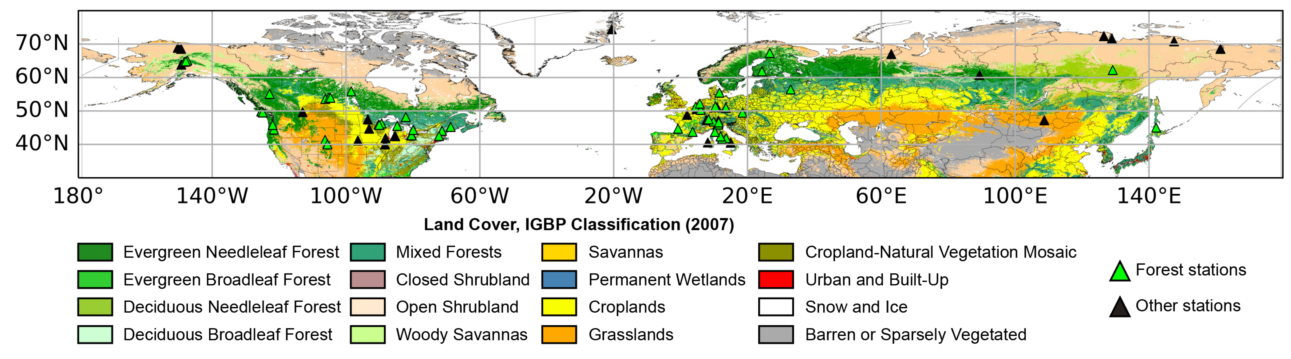
2.2. Selecting FLUXNET Stations for Flux Data Analysis

In our study, we examined the influence of extreme weather conditions on CO₂ and latent heat fluxes in boreal and temperate forest ecosystems. The boreal and temperate forest biomes cover significant areas north of 40° N, with diverse climatic and landscape conditions. The observed global increase in the frequency of extreme weather events varies across regions, affecting natural ecosystems and CO₂ and latent heat fluxes in different ways. In order to highlight the response of forest ecosystems to extreme weather events (temperature, precipitation), we focused on the areas with the most significant increase in frequency.

The 95% quantile of the power density function (PDF) was chosen as the threshold for extreme values of meteorological parameters. The PDFs were calculated separately for each month of the year to exclude the influence of the seasonal cycle and then averaged over the period from 1979 to 2021. The normal distribution for temperature and the Weibull distribution for precipitation were used, which were found to be the most appropriate for the continents [47]. For each grid point of the ERA5 reanalysis located on the continent north of 40° N, the number of months in the reference period (1979–2021) in which the temperature or precipitation exceeded (does not reach) the 95% (5%) quantile was calculated. The changes in this number during the last few decades were then estimated.

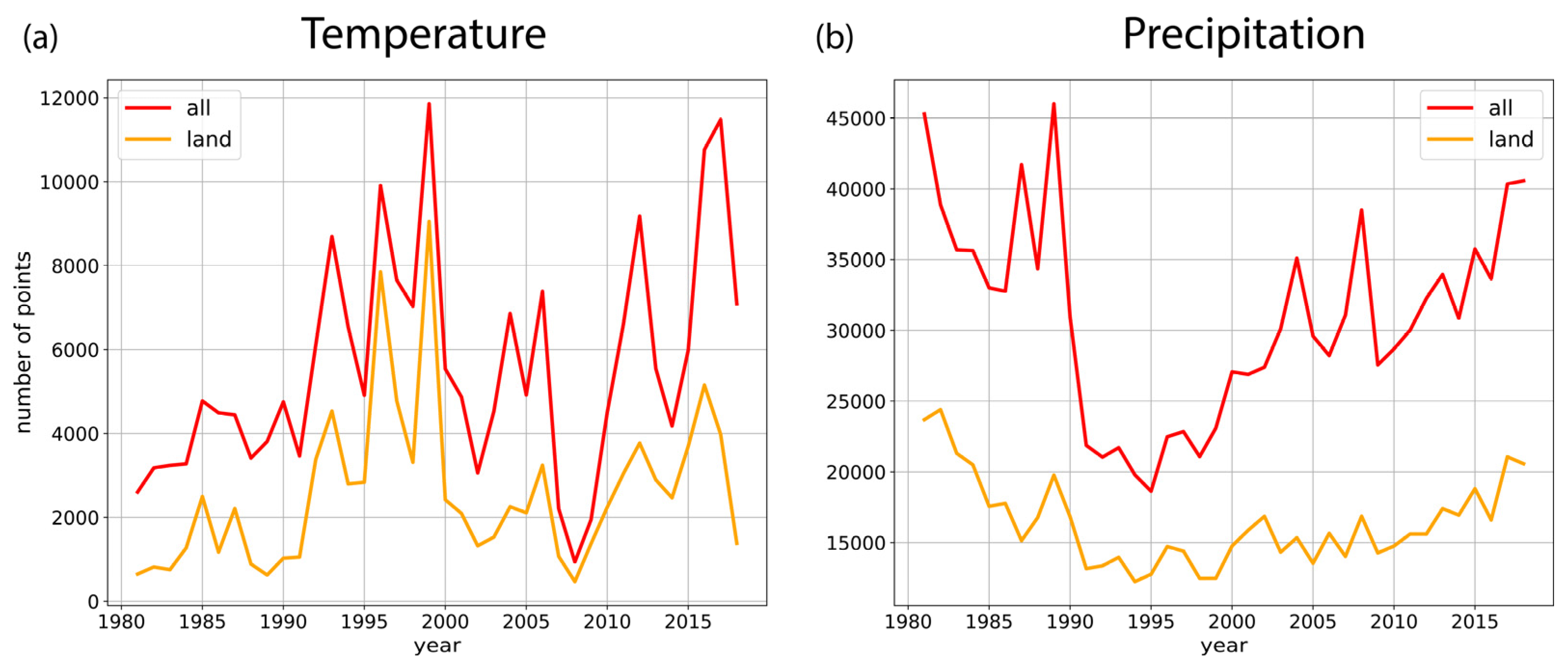
2.2.1. Statistical Analysis of Temperature and Precipitation Trends

To compare the frequency of extreme weather conditions at the end of the 20th century and the beginning of the 21st century, two periods were selected. To define these periods, we first analyzed the trend changes in the temperature and precipitation time series. The sequential version of the Mann–Kendall test statistic (SeqMK-test) [48,49,50] was used. This method can be used to determine whether a time series has a monotonic upward or downward trend. It can also be used to identify trend turning points in time series (e.g., air temperature and precipitation). The details are provided in the Supplementary Materials (S2).

For each year of the study period, we calculated the total number of grid cells in the entire land area north of 40° N with trend turning points (Figure 1). The number of trend turning points in each grid cell is shown in Figure 2. For air temperature, most of the trend turning points occurred in 1996 and 1999 (Figure 1a). For precipitation, the trend turning points occurred most frequently in the 1980s. However, they were more evenly distributed over the period (Figure 1b), and the number of trend turning points was much larger than for air temperature (Figure 2). Despite the identified trend changes in individual grid cells and regions, it was difficult to identify a unique trend turning point for the entire territory of the mid- and high latitudes of the Northern Hemisphere, especially for precipitation. Taking into account that for air temperature the maximum grid cells had a trend turning point at the end of the 20th century, we decided to divide the analyzed period into two equal time intervals (1980–2000 and 2001–2021), which were considered to characterize the average climate conditions of the late 20th and early 21st century.

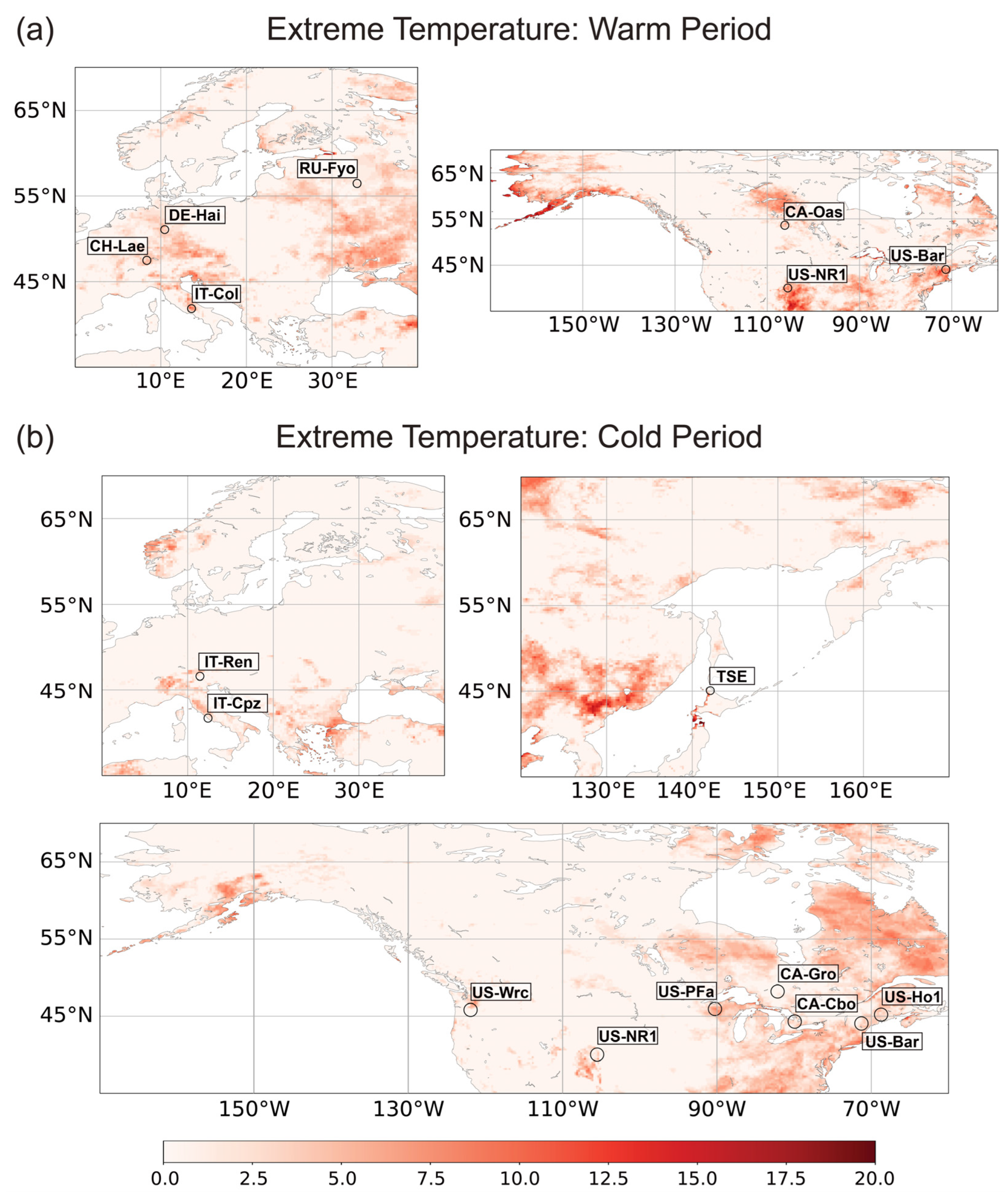
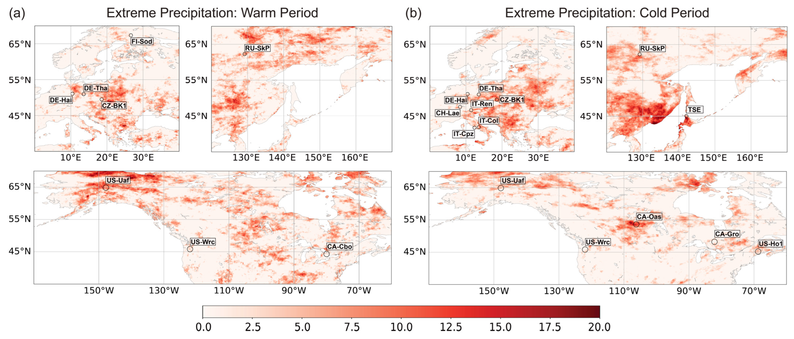
2.2.2. Selecting FLUXNET Stations for Analysis of Flux Response to Extreme Weather Conditions

For the selected periods, the number of months in which temperature or precipitation exceeded the 95% quantile was calculated separately for the warm (April–September) and cold (October–March) seasons. The difference between the late 20th and early 21st centuries is shown in Figure 3 for air temperature and Figure 4 for precipitation. The regions with a significant increase in the number of extremes are marked by an intense red color.

A total of 18 flux stations from the entire global and regional FLUXNET archives (Figure 5) were selected to analyze the possible NEE and LE flux feedback of temperate and boreal forests for extreme temperature and precipitation events, corresponding to the regions with the highest increase in the number of extreme temperature (Figure 3) or precipitation (Figure 4) events over the last few decades. Furthermore, eight additional stations with very long and gap-free flux observation series and a consistently high frequency of occurrence of anomalous weather events were also chosen. All stations were assigned to 5 major vegetation types [51] according to the ecosystem classification used in the FLUXNET archives: evergreen needleleaf, evergreen broadleaf, deciduous needleleaf, deciduous broadleaf, and mixed forests (Figure 6b). The selected flux monitoring stations are associated with various climate types according to the Köppen climate classification [52] (Figure 6a). The information on the location of the flux stations, the period of observation, the types of climate, and the characteristics of the forests are summarized in the

Table 1. The FLUXNET forest stations selected for analysis of flux response to extreme weather conditions.

Stations	Long, Lat	Elev. (m)	Vegetation Type IGBP	Climate Type	Forest Species Composition	Age (Years)	Height (m)	Period
(1) BE-Bra	51.31° N, 4.52° E	16	Mixed forests	Cfb, temperate oceanic	Pinus sylvestris, Quercus robur	94	21	1999–2014
(2) CA- Gro	48.22° N, 82.16° W	340		Dfb, warm summer humid continental	Populus tremuloides, Picea marian, Picea glauca, Betula papyrifer, Abies balsame	93	31	2003–2014
(3) CH- Lae	47.48° N, 8.36° E	689		Dfb, warm summer humid continental	Picea abies, Fagus sylvatica, Fraxinus excelsior, Acer pseudoplatanus	52–185	30.6	2004–2014
(4) US- PFa	45.95° N, 90.27° W	470		Dfb, warm summer humid continental	Populus grandidentata, Betula pendula, Acer rubrum, Tilia tomentosa, Alnus incana	110– 120	24	1996–2022
(5) TSE: Teshio CC-LaG	45.06° N, 142.11° E	70	Conifer–hardwood mixed forest	Dfb, warm summer humid continental	Quercus crispula, Betula ermanii, Betula platyphylla var. japonica, Abies sachalinensis, Picea jezoensis	175	18–25	2001–2002
(6) CA- Oas	53.63° N, 106.20° W	530	Deciduous broadleaf forests	Dfc, subarctic	Populus tremuloides, Populus balsamifera, Corylus cornuta, Alnus crispa	104	22	1996–2010
(7) DE- Hai	51.08° N, 10.45° E	430		Dfb, warm summer humid continental	Fagus sylvatica, Fraxinus excelsior, Acer pseudoplantanus, Acer plantanoides, Carpinus betulus	250	33	2000–2012
(8) DK- Sor	55.49° N, 11.64° E	40		Cfb, temperate oceanic	Fagus sylvatica	102	25.8	1996–2014
(9) IT-Col	41.85° N, 13.59° E	1560		Cwa, monsoon-influenced humid subtropical	Fagus sylvatica	90	20.2	1996–2014
(10) US-Bar	44.06° N, 71.29° W	272		Dfb, warm summer humid continental	Fagus grandifolia, Acer saccharum, Betula alleghaniensis, Betula papyrifera, Tsuga canadensis	120	19	2004–2017
(11) CA- Cbo	44.32° N, 79.93° W	120		Dfb, warm summer humid continental	Acer rubrum, Pinus strobus, Populus grandidentata, Fraxinus americana	107	22	1995–2020
(12) CZ- BK1	49.50° N, 18.54° E	875	Evergreen needleleaf forests	Dfb, warm summer humid continental	Picea abies	27	12	2004–2014
(13) DE- Tha	50.96° N, 13.56° E	385		Cfb, temperate oceanic	Picea abies, Betula pendula, Larix decidua, Pinus sylvestris	136	25	1996–2014
(14) FI-Hyy	61.85° N, 24.29° E	181		Dfc, subarctic	Pinus sylvestris	80	14	1996–2014
(15) FI-Sod	67.36° N, 26.64° E	180		Dfc, subarctic	Pinus sylvestris	100	12.7	2001–2014
(16) IT-Ren	46.59° N, 11.43° E	1730		Cfb, temperate oceanic	Picea abies, Pinus cembra, Larix decidua	90	29	1998–2013
(17) RU- Fyo	56.46° N, 32.92° E	265		Dfb, warm summer humid continental	Picea abies, Betula pubescens	150	15	1998–2014
(18) US- NR1	40.03° N, 105.55° W	3050		Dfc, subarctic	Abies lasiocarpa, Picea engelmannii, Pinus contorta	118	18	1998–2014
(19) CA- LP1	55.11° N, 122.84° W	751		Csa, hot summer Mediterranean	Pinus contorta	97	15	2007–2021
(20) CA- Ca3	49.53° N, 124.90° W	170		Cfb, temperate oceanic	Pseudotsuga menziesii, Thuja plicata, Abies grandis	35	8	2001–2021
(21) US- Ho1	45.20° N, 68.74° W	60		Dfb, warm summer humid continental	Picea rubens, Pinus strobus, Tsuga canadensis	130	20	1996–2020
(22) US- Uaf	64.87° N, 147.86° W	155		Dwc, monsoon-influenced subarctic	Picea mariana	85	3	2003–2021
(23) US- Wrc	45.82° N, 121.95° W	371		Csb, warm summer Mediterranean	Picea rubens, Tsuga canadensis	500	60	1999–2015
(24) IT-Cpz	41.70° N, 12.38° E	68	Evergreen broadleaf forests	Csb, warm summer Mediterranean	Quercus ilex	100	10	1997–2009
(25) FR- Pue	43.74° N, 3.60° E	270		Csa, hot summer Mediterranean	Buxus sempervirens, Quercus ilex	129	19	2000–2014
(26) RU- SkP	62.26° N, 129.17° E	246	Deciduous needleleaf forests	Dfc, subarctic	Larix, Salix, Betula pendula	190	20	2012–2014

.

2.3. Data Analysis

Daily means for air temperature were calculated from 3 h and 30 min reanalysis and flux site data sets, respectively. Daily precipitation was calculated as the daily sum of 1 h and 30 min precipitation data from reanalysis and flux sites, respectively. Temperature anomalies were calculated by removing the daily mean, calculated for the period from 1991 to 2021.

In order to account for the delayed response of few-day wet spells as well as the impact of prolonged drought on NEE and other components of the carbon budget, we additionally used the antecedent precipitation index (API) in our study. In our case, this index can be an indicator of soil moisture deficiency or surplus and therefore may be the best indicator to describe the influence of precipitation on CO₂ fluxes and evapotranspiration.

To calculate the API for each day of the year at the flux station, we followed Kohler and Linsley [53] and Li et al. [54]:

$$API={\displaystyle {\sum }_{t=1}^M{P}_t} k^t$$

(1)

where P_t is the precipitation in the tth antecedent day, M is the statistical number of antecedent days, and k is the decay constant. In our study, we assumed that M is equal to 14 days and k is equal to 0.8.

Mean daily NEE and LE rates for each station were calculated by averaging 30 min flux data sets. The gaps in the flux time series, caused by equipment and power failures, weak turbulence, heavy rainfalls, etc., for all selected flux stations were filled out in our study using the REddyProc package [55] and the algorithms described by Reichstein et al. [56]. The method was applied by taking into account the locations of most of the selected flux stations in mid-latitudes between 40° N and 55° N, where this method provides reasonable estimates [55] and does not produce the systematic bias in daily flux estimates that it does in high latitudes [57]. The choice of method was also influenced by the simplicity and robustness of its application for filling in gaps in experimental data series, although it may be less accurate compared to more complex approaches based on process-based mathematical modeling [58] and machine learning techniques [57]. Daily anomalies of NEE and LE were calculated as the difference between the daily and monthly means of NEE and LE over the available observation period at each station.

Extreme temperature periods were defined as periods when the daily mean temperature anomaly exceeded the 95% quantile (for extremely high temperatures) or did not reach the 5% quantile (for extremely low temperatures) of the probability density function (PDF) [45]. The normal distribution for air temperature was used in our study as the most appropriate for long-term time series analysis [47]. The PDFs were calculated for each calendar month of the observation periods and averaged over the period from 1991 to 2021.

Two approaches were used to analyze the effect of precipitation variability on NEE and LE fluxes. In the first approach, extremely heavy precipitation days were identified as days with daily precipitation exceeding the 95% quantile of the power density function, using the Weibull distribution for precipitation [47]. This method allows to highlight the immediate response of the ecosystem to heavy precipitation to be highlighted, which is mostly associated with increased soil respiration resulting in high CO₂ emissions. However, this approach is not suitable for identifying the effect of a precipitation deficit on NEE and LE fluxes, because the lack of precipitation during one or several days in mid-latitudes cannot be considered a stress condition for NEE and LE fluxes in temperate and boreal forests. The effect of sufficient or deficient soil moisture may be more important for NEE and LE fluxes than the effect of the presence or absence of precipitation. Soil moisture depends on the cumulative effect of precipitation, which can be estimated using the API index. Therefore, we used the second approach to determine the sensitivity of NEE and LE to precipitation based on the API index.

Extremely high daily API anomalies were defined as anomalies above 1 standard deviation (STD) of available time series at each station. To eliminate the influence of the seasonal cycle, the STD was calculated separately for each calendar month. The threshold for extremely low API is the 5% threshold of the time series amplitude. The amplitude was defined as the difference between the mean maximum and mean minimum API for each calendar month averaged over the period 1991–2021. The STD threshold is not suitable for low API because the STD is often greater than the mean API for a specific month, and therefore, the values below −1 STD are negative, which is impossible for precipitation.

The extremely high (low) NEE and LE flux anomalies were defined as exceeding 1STD (−1 STD) of the total time series for each calendar month separately.

The quantile thresholds were not applied to fluxes and API because their PDF types varied significantly between ecosystem types, making it difficult to select the type of theoretical distribution to approximate the empirical distribution of the data sets. In addition, the short time series for ecosystem fluxes at several stations also made it difficult to determine the appropriate theoretical PDF.

To analyze the relationships between temperature/precipitation and NEE/LE anomalies, we first focused on the temporal variability of weather conditions (temperature and precipitation) and associated NEE and LE flux anomalies. As an example, Figure S3 in the Supplementary Materials shows the temporal variability of daily temperature anomalies, precipitation amount, API, and NEE and LE flux anomalies for the forest station located in the evergreen needleleaf forest of western Canada (CA-Ca3).

To quantify the relationships between the weather extremes and flux anomalies, we calculated the percentage of days when the NEE or LE anomaly exceeded the STD values while the temperature/precipitation exceeded the 95% quantile for the upper threshold or the temperature (API) did not reach the 5% quantile (was lower than 5% of the amplitude) for the lower threshold. The percentage was calculated from the total number of days on which one of the characteristics (temperature anomaly, daily precipitation, or API) exceeded the threshold. Positive NEE anomalies are associated with increased CO₂ emissions, whereas negative anomalies are associated with enhanced CO₂ uptake. The positive/negative LE anomalies are associated with increased/decreased evaporation. The cases for which the total number of days above the threshold for temperature/precipitation and fluxes was less than 10 days were excluded from the data analysis.

3. Results and Discussion

3.1. The Response of NEE and LE Fluxes to the Extreme Temperature Anomalies

The responses of NEE and LE fluxes to temperature changes in temperate and boreal forests show a wide range of variation across different landscapes and over time due to plant species characteristics, growing conditions, plant age, and adaptation to changing environmental conditions. Intra-annual variability is determined by seasonal changes in green plant biomass, as well as by differences in assimilation processes occurring in woody plants during cold and warm periods. Overall, during the cold season, plant photosynthesis is completely shut down in deciduous forests, and it is strongly inhibited in evergreen forests. During the growing season, in the warm half of the year, photosynthesis and respiration of plants increase significantly under favorable temperature, solar radiation, and soil moisture conditions for plant growth for both evergreen and deciduous tree species after the appearance of leaves. Anomalous weather conditions can affect tree functioning and growth, resulting in changes in NEE and LE fluxes.

In order to highlight the specific response of woody plants under different growing conditions in different seasons to anomalous weather conditions, we considered the response of forest ecosystems to external forcing in the warm and cold seasons separately. The beginning and end of the warm season are associated with a steady transition of the mean daily temperature through zero for at least seven consecutive days. For several stations located in warm climates with prevailing positive temperatures (e.g., station in the Mediterranean region), the seasonal transition was determined by the sharp change in gross primary production (GPP) values observed during leaf emergence and leaf fall.

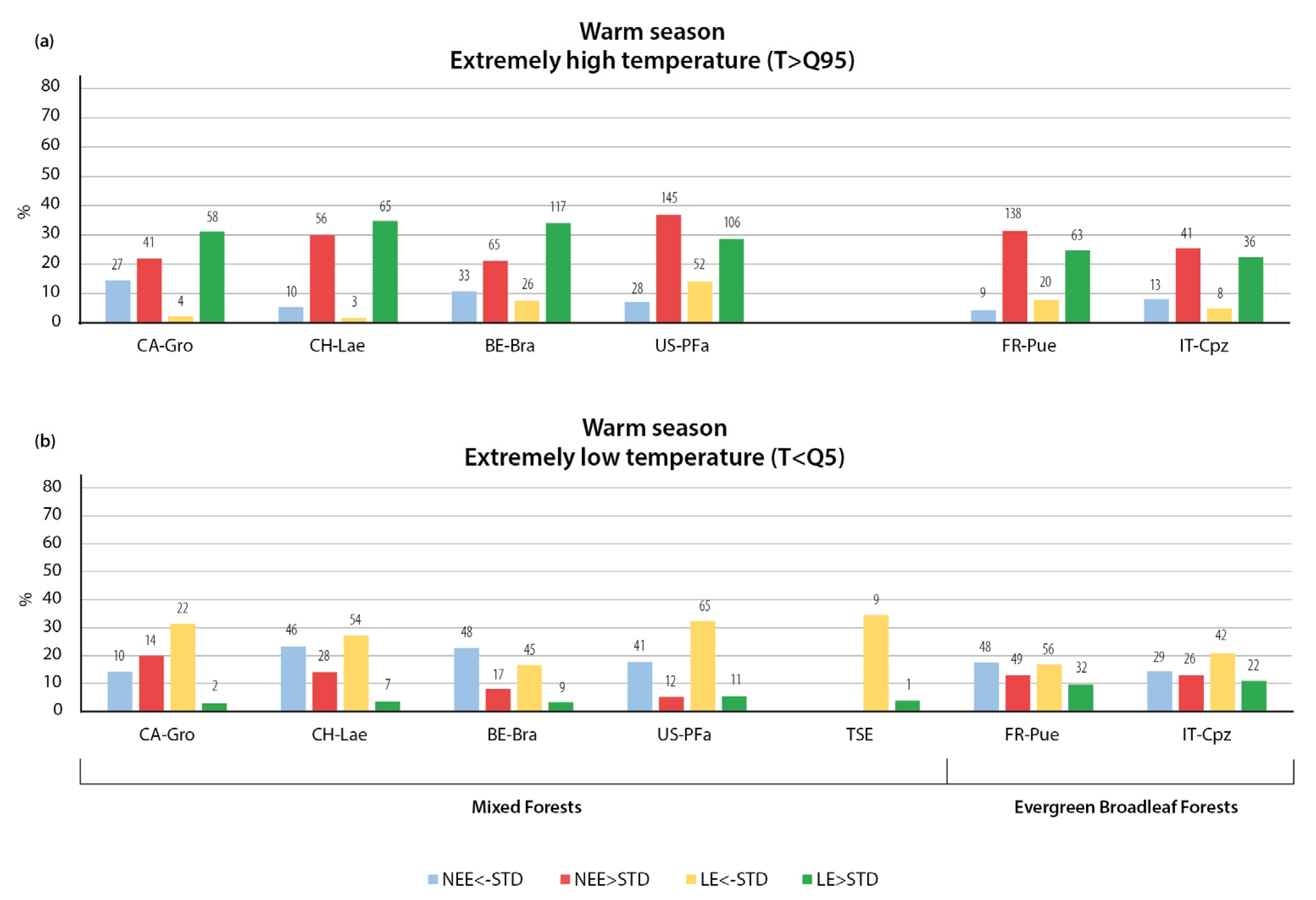
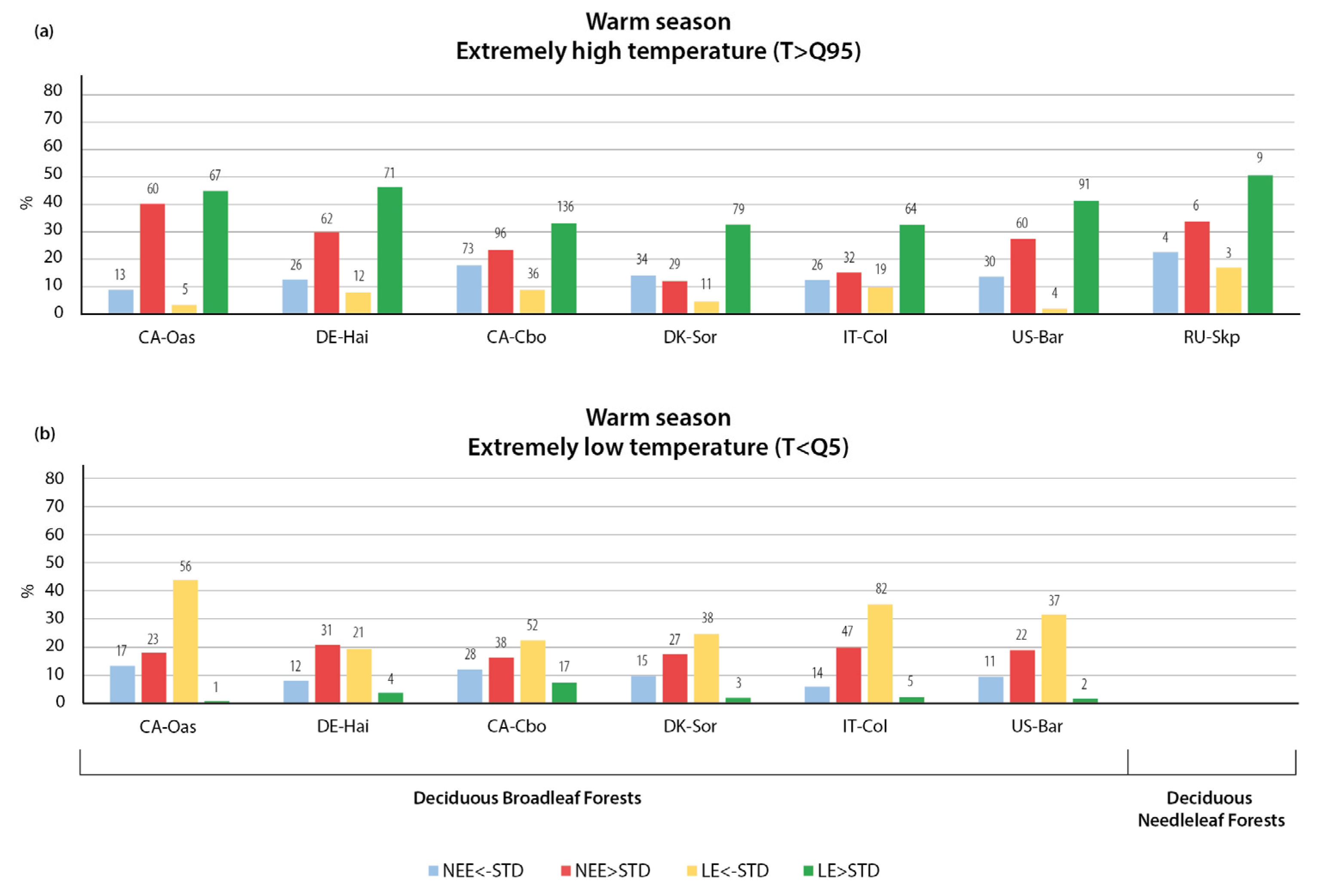
3.1.1. Variation in NEE and LE Flux in Warm Season

In all considered forest types and forest ecosystems during the warm season, extremely hot conditions (temperature anomalies exceeding the 95% quantile) were mostly associated with increased CO₂ release into the atmosphere (positive NEE anomalies exceeding STD are presented by red bars in Figure 7, Figure 8, Figure 9 and Figure 10; positive trends in NEE anomalies with increasing temperature are also shown in Figure S4.1). There was also a tendency for the NEE anomaly to decrease as the temperature anomaly increased for most stations (Figure S5.1). The highest percentage of hot days accompanied by a positive NEE anomaly exceeding STD (up to half of all hot days) was observed in the evergreen coniferous forests (Figure 7a). Extremely high temperatures stressed photosynthesis and reduced the GPP rate of forest ecosystems. As a result, more CO₂ was released into the atmosphere. It is noteworthy that the negative NEE anomalies (blue bars) also occurred during the hot periods (Figure 7a), but the percentage of days with them was much lower (6–15%). The increase in temperature anomaly was accompanied by a prevailing decrease in CO₂ uptake or an increase in CO₂ release (Figure S5.2). Exceptions are two stations located in Finland (FI-Hyy) and the United States (US-NR1), where the probability of positive and negative NEE anomalies was almost equal. The Niwot Ridge experimental site (US-NR1) is located in a subalpine forest ecosystem at an elevation of 3050 m [59]. The Hyytiala site (FI-Hyy) is located in a homogeneous 60-year-old pine (Pinus sylvestris L.) forest stand [60]. Sufficient soil moisture conditions due to uniform precipitation distribution throughout the year, including the period of strong positive temperature anomalies, may be a key reason for the equal probability of positive and negative NEE anomalies observed during extremely high temperatures.

The inverse response of NEE to high temperature was found at the evergreen coniferous forest station Bily Kriz in the Czech Republic (CZ-BK1). The dominant tree species in the forest is the 40-year-old Norway spruce (Picea abies (L.) Karst) [61]. The results show that in the forest, higher CO₂ uptake (blue bar) occurred more often during the hot periods (Figure 7a). The Bily Kriz forest site is located in a hilly region (elevation about 900 m above sea level) and is characterized by a relatively high amount of annual precipitation (>1300 mm), which provides sufficient soil moisture conditions and may ensure low sensitivity of young forest stand to positive temperature anomalies [62].

In mixed forests and evergreen broadleaf forests (Figure 8a), as well as in deciduous broadleaf and needleleaf forests (Figure 9a), positive NEE flux anomalies above STD, corresponding to high CO₂ release, also dominated under extremely high temperatures, but the percentage of days was lower. The lower effect of high temperatures on plant photosynthesis and CO₂ uptake in these forests compared to the evergreen needleleaf forests may be due to the higher sensitivity and vulnerability of dark coniferous forest stands to higher temperatures and positive temperature anomalies [9,63,64,65,66]. Thus, it can be expected that the mixed and broadleaf tree species had higher drought and heat tolerance and were less sensitive to heat anomalies. This may be the reason why the NEE anomalies at the DK-Sor [67] and It-Col (deciduous broadleaf forest) [68] sites were evenly distributed and a positive temperature anomaly led to both increased CO₂ uptake (blue bars) and increased CO₂ release (red bars) (Figure 8a and Figure 9a).

Extremely high temperatures were also accompanied by positive anomalies of LE (green bars in Figure 7, Figure 8, Figure 9 and Figure 10) due to the intensification of evaporation processes with increasing temperature. This relationship was observed in all forest types considered (Figure 7a, Figure 8a and Figure 9a). At the same time, as shown in Figure S4.2, the temperature increase led to growth in LE anomalies. Negative LE anomalies (yellow bars in Figure 7, Figure 8, Figure 9 and Figure 10) during the hot periods were very rare (less than 10% of days). The cold periods occurring during the warm season mostly induced strong negative LE anomalies (Figure 7b, Figure 8b, and Figure 9b) due to the suppressed evaporation at low temperatures [69]. The temperature decrease resulted in a reduction in negative LE anomalies (Figure S4.2).

The response of NEE fluxes to negative temperature anomalies varied significantly among forest types and even among forests within a forest biome, depending on forest species composition, forest location, and landscape characteristics (Figure 7, Figure 8 and Figure 9, Figures S5.3 and S5.4).

At three stations located in mixed forests and at the FR-Pue station, located in evergreen broadleaf forests (Figure 8b), CO₂ uptake (blue bars) increased with decreasing temperature, indicating more favorable conditions for photosynthesis at relatively low summer temperatures. However, positive NEE anomalies, associated with higher CO₂ release (red bars), occurred more frequently than negative ones at most of the stations located in evergreen coniferous forests (Figure 7b) and in deciduous broadleaf and needleleaf forests (Figure 9b). This effect may lead to several causes and may be closely related to local microclimate and soil moisture conditions [19].

Thus, the positive and negative temperature anomalies in both evergreen coniferous forests and deciduous broadleaf and needleleaf forests resulted in prevailing positive NEE anomalies. The temperature effect on NEE and LE fluxes during the warm season did not differ significantly between boreal and temperate forests, with similar controlling mechanisms involved. Under positive temperature anomalies, it may be determined by suppressed assimilation processes due to high temperature and insufficient soil moisture [70,71,72], as well as a higher decomposition rate of soil organic matter and higher autotrophic respiration [21]. Under negative temperature anomalies, it may be caused by a large reduction in GPP at lower temperatures [73].

Comparing the effect of positive and negative temperature anomalies on NEE and LE, we can see that extremely high temperatures had a stronger effect on NEE and LE fluxes than air temperature decreases during the warm season (Figure 8 and Figure 9). This suggests that heat waves may be the most important drivers of CO₂ and H₂O budgets in temperate and boreal forests. It is noteworthy that drought can also have a very strong impact on forest ecosystems, but in this study we did not directly consider the effect of drought, as drought is a much more complex ecological event than just the precipitation deficit analyzed in this study.

3.1.2. Variation in NEE and LE Flux in Cold Season

The influence of temperature anomalies on NEE of forest ecosystems during the cold season was mainly manifested by changes in the ecosystem respiration rate depending on the air temperature oscillation. The anomalies of the LE were also closely related to the variations of the temperature and the solar radiation. The number of considered forest ecosystems was reduced to 21, because at 5 out of 26 considered stations there was no possibility to detect the cold season because the duration of the period with negative temperatures never exceeded 7 days.

In the evergreen needleleaf forests, the strong NEE and LE anomalies (exceeding STD) occurred rather rarely during extremely cold periods; at most stations, less than 10% of extremely cold days were characterized by extreme flux anomalies (Figure 7d). This may be the result of a general weakening of the CO₂ and H₂O fluxes during the winter months. The thaws (temperature higher than 95% quantile) mostly caused increased CO₂ emissions (red bars on Figure 7c) due to intensified ecosystem respiration. The results are in good agreement with recent findings of increased CO₂ release in northern permafrost regions during winter, which has accelerated recent Arctic warming and permafrost thawing [74,75].

In other forest types south of evergreen coniferous forests, extremely low temperatures mostly led to negative NEE anomalies (blue bars in Figure 10b), whereas high temperatures mostly led to positive NEE anomalies (red bars in Figure 10a). Soil respiration was expected to be a major driver of ecosystem fluxes in winter [76,77].

The decreased evaporation (yellow bars) was associated with more than 20% of the days with extremely low temperatures at 6 out of 21 stations, whereas at other stations, the anomalies were minimal (Figure 7d and Figure 10b). On the contrary, the periods of winter temperature increase more often resulted in positive anomalies of LE (green bars in Figure 7c and Figure 10a), which was the common feature for warm and cold seasons.

3.2. The Response of NEE and LE Fluxes to Extreme Precipitation

Since the precipitation characteristics (type, intensity, duration, etc.) are drastically different between the warm and cold seasons, and thus may induce different responses in NEE and LE fluxes, we analyzed the warm and cold seasons separately. The identification of the periods was the same as in the previous section describing the influence of extreme temperatures. Two characteristics of the precipitation regime were used for the analysis: the daily precipitation amount, which characterizes the immediate effect of heavy rains on NEE and LE fluxes, and the API index, which captures the prolonged cumulative precipitation effect.

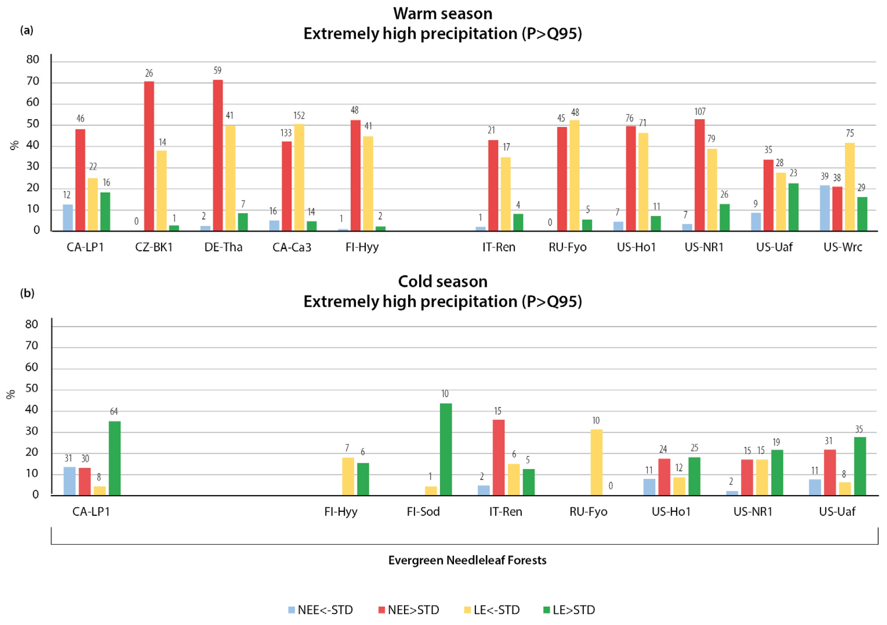
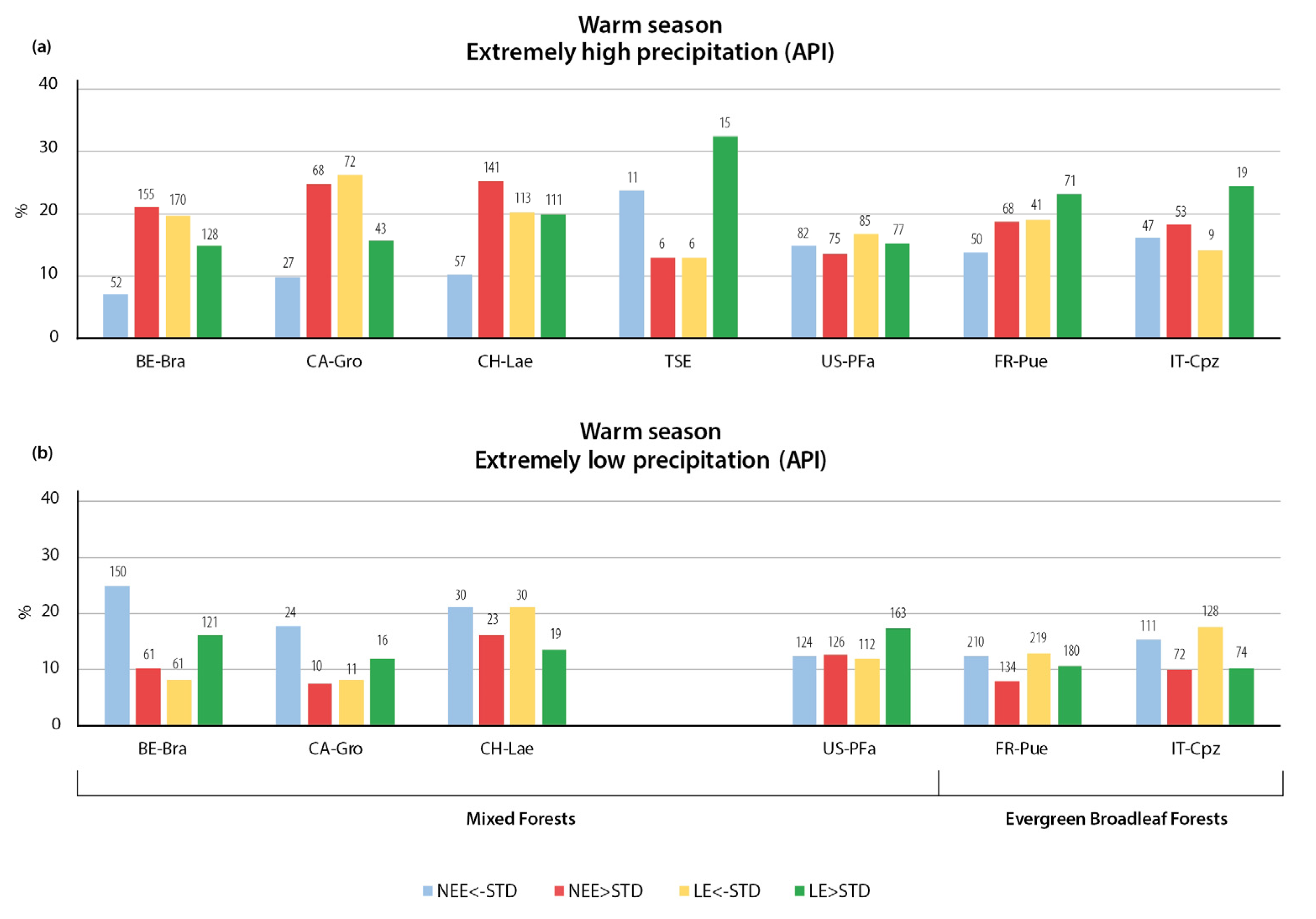
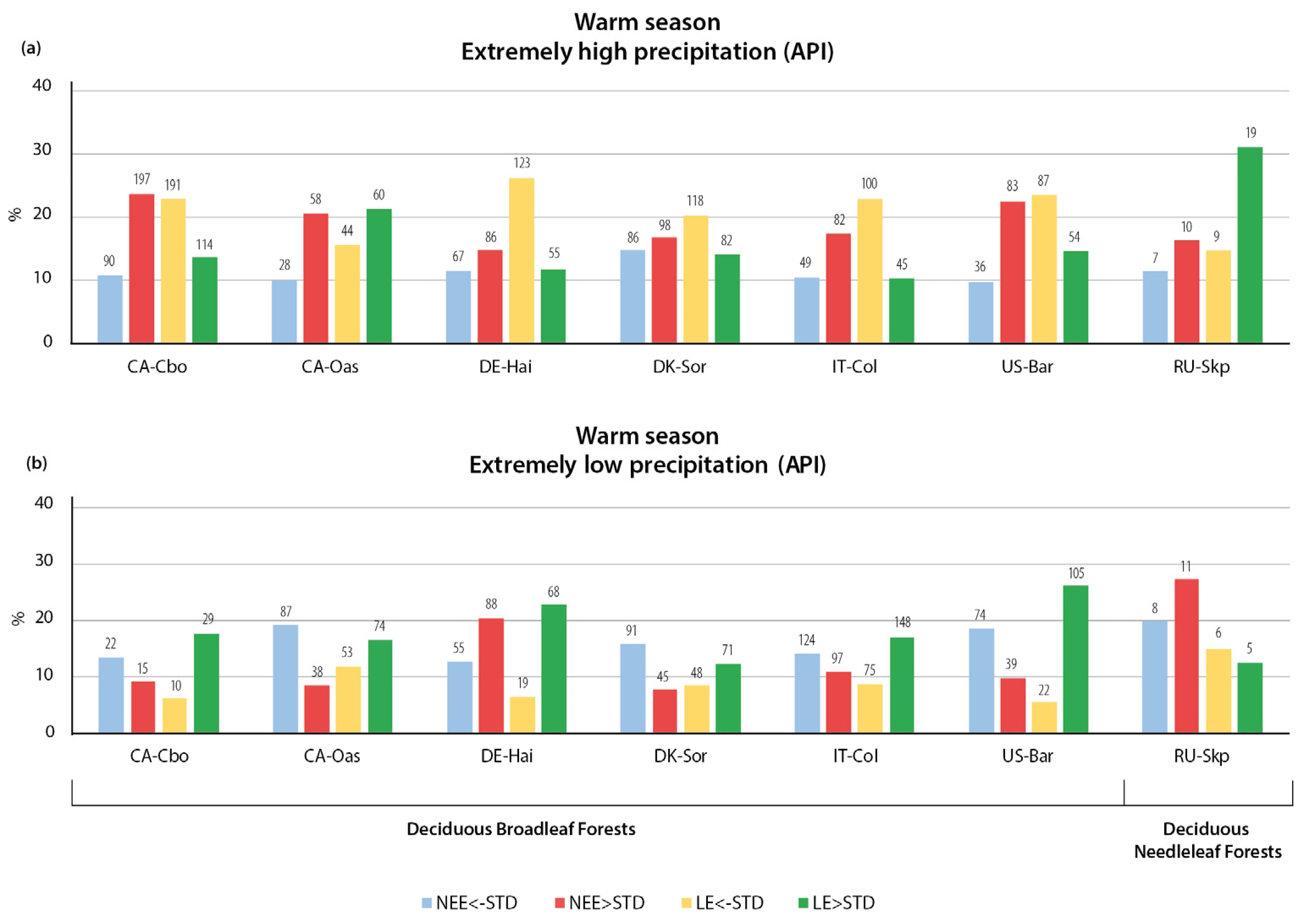
3.2.1. Variation in NEE and LE Flux in Warm Season

In almost all forest types considered in our study, heavy precipitation led to increased CO₂ emissions into the atmosphere (red bars in Figure 11, Figure 12, Figure 13, Figure 14, Figure 15 and Figure 16). There was also a slight increase in the NEE anomaly with increasing precipitation (Figure S6.1). In the mixed evergreen needleleaf and broadleaf forests, up to 40–70% of days with extreme precipitation were associated with positive NEE anomalies above STD (Figure 11a and Figure 12a). In deciduous forests, the percentage was slightly lower: 30–50% (Figure 12b). The observed response may be related to the well-known “Birch effect” [34], which is manifested by a strong CO₂ release after rewetting of dry soils, resulting from increased soil moisture and enhanced decomposition and mineralization rates.

The prolonged effect of soil wetting on NEE fluxes was estimated using the API index. It was more often associated with strong negative NEE anomalies (blue bars) than with extreme daily precipitation. Although CO₂ emissions (red bars) exceeded CO₂ uptake (blue bars) in mixed (Figure 14a) and evergreen needleleaf forests (Figure 13a), as well as in deciduous broadleaf and needleleaf forests (Figure 15a), the difference between the percentage of days with positive and negative anomalies was rather small (between 2 and 20%). Negative and positive NEE anomalies were evenly distributed during days with extreme API values in evergreen broadleaf forests (Figure 14a). The increase in CO₂ uptake during the period following heavy precipitation (API in our study was calculated as the weighted total precipitation for the preceding 14 days) was due to intensified photosynthesis in living plants in the case of sunny weather and sufficient soil moisture conditions [78].

The precipitation deficit, represented by extremely low API values, was associated with high CO₂ uptake in most considered forest ecosystems. In the absence of prolonged soil drought, this trend demonstrated the high adaptive potential of the most temperate and boreal forest ecosystems to adapt to short-term (less than 14 days) periods without precipitation.

The evergreen needleleaf forests had high CO₂ uptake during the warm season for 9–28% of the days with low API (blue bars in Figure 13b). Positive NEE anomalies (red bars) occurred more frequently than negative ones during the dry periods in only two evergreen needleleaf forests in North America: a black spruce forest in Alaska (US-Uaf) [79] and an over-mature Douglas fir/western hemlock forest (US-Wrc) [80]. In both ecosystem types, the high sensitivity of conifers to a lack of precipitation can be explained by the low adaptive capacity of woody plants to soil drought, e.g., due to the shallow root system. Such an effect may also be due to the low water storage capacity of the soil horizons or a number of other reasons. In the black spruce forest, this phenomenon was due to permafrost, whereas in the Douglas fir/western hemlock forest, it can be attributed to hilly topography and high runoff. High CO₂ uptake during dry periods was observed in all evergreen, deciduous, and mixed forests studied (blue bars in Figure 14b and Figure 15b), except for coniferous broadleaf mixed forests in the northernmost part of Japan. This was apparently due to the higher resistance of mixed forest stands to drought events compared to monospecific forests [81,82].

In the larch (needleleaf deciduous) forest, the lack of precipitation resulted in higher CO₂ emissions (positive NEE anomaly) (red bars in Figure 15b), indicating stressed photosynthesis caused by a lack of precipitation and reduced soil wetness.

In most of the analyzed temperate and boreal forests, heavy precipitation was associated with strong negative LE flux anomalies (yellow bars in Figure 11, Figure 12, Figure 13, Figure 14, Figure 15 and Figure 16), indicating suppressed evaporation due to the high water vapor pressure in the air during and after precipitation, as well as reduced incoming solar radiation due to cloudy weather (Figure 11a and Figure 12a,b). The observed positive LE anomalies were associated with increased evaporation after precipitation events due to both increased plant transpiration and interception evaporation (Figure S6.3) [83].

The effect of an extremely high API index on LE was almost opposite to the effect of extremely high precipitation on LE, indicating the strong difference between the evaporation response to the instantaneous and prolonged effect of soil wetting. On days with heavy precipitation, the air is usually highly saturated with water vapor, and clouds reduce incoming solar radiation, which also significantly limits the rate of evapotranspiration. On the other hand, after periods of heavy precipitation, transpiration and evaporation rates can be relatively high due to sufficient soil moisture, especially under warm and sunny weather conditions [84].

In the evergreen needleleaf forests at 6 (Ca-Ca3, Ca-LP1, FI-Sod, IT-Ren, US-NR1, US-Uaf) of 11 flux stations, the increase in evapotranspiration was more frequent during wet periods—up to 29% of the days in which API > STD were characterized by positive anomalies of LE fluxes (green bars in Figure 13a), and the dry periods resulted in weaker evaporation (yellow bars in Figure 13b) in only 4 of 6 flux stations (Ca-LP1, FI-Sod, US-NR1, US-Uaf). Obviously, the soil moisture completely controls the intensity of LE fluxes in the atmosphere. However, in the Douglas fir forest in Canada (Ca-Ca3) [85] and in the mountainous spruce forest in Italy (IT-Ren) [86], positive LE anomalies (green bars) dominated on days with both extremely low and high API. The Italian spruce forest was unevenly aged, with a high proportion of old trees. Several studies have shown that such older stands tend to be more resilient to climate stress than managed younger forests [12].

At five stations located in the evergreen coniferous forests (Figure 13a), reduced evapotranspiration (yellow bars) occurred during wet periods (up to 28% of days with strong negative LE anomalies). The opposite LE anomalies were associated with a precipitation deficit (Figure 13b) at these stations (with the exception of the spruce forest in European Russia, Ru-Fyo [87,88]), with increased evaporation (green bars) under dry conditions (small API). This was probably due to changes in net radiation, as rainy periods are usually associated with cloudy weather and decreased incoming solar radiation, whereas dry conditions coincide with high incoming radiation.

In the mixed forests of Belgium (Be-Bra) and Canada (Ca-Gro) and deciduous and evergreen broadleaf forests (US-Pfa), high API values were associated with decreased evapotranspiration (yellow bars in Figure 14a and Figure 15a), whereas low API values were associated with increased evapotranspiration (green bars in Figure 14b and Figure 15b). It is noteworthy that the difference between negative and positive anomalies was rather small. In the deciduous needleleaf (Ru-Skp) and broadleaf forests of Italy and France, wet periods were accompanied by strong (green bars in Figure 15a) and dry periods of weak evaporation (yellow bars in Figure 15b). In the first case, the net radiation likely had a more significant effect on LE, whereas in the second case, it was the soil moisture. In the mixed forest of Japan (TSE) [89], increased evapotranspiration dominated, with no apparent dependence on the API index (Figure 14a,b).

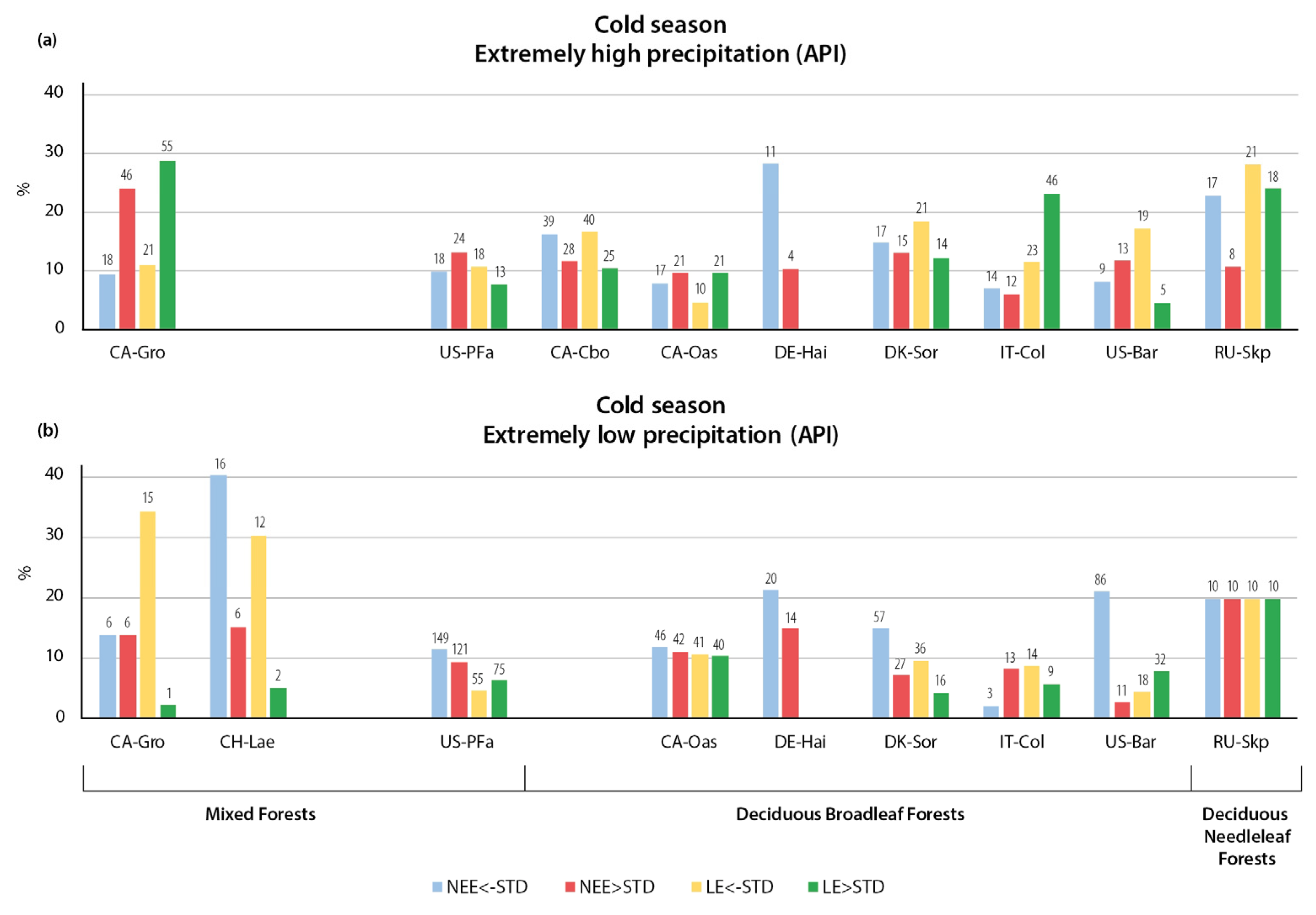
3.2.2. Variation in NEE and LE Flux in Cold Season

In contrast to the warm season, when precipitation has both direct and indirect effects on CO₂ and H₂O fluxes through changes in soil moisture content that affect GPP and RE, plant transpiration, and soil evaporation, during the cold season in boreal and temperate forests under negative temperatures and permanent snow cover, the physical and biological mechanisms of both direct and indirect effects of precipitation on CO₂ and H₂O fluxes are completely absent. During the cold season, the response of CO₂ and H₂O fluxes to anomalous precipitation and API can only be expected at the beginning and the end of the cold season, before and after the establishment of permanent snow cover and while the ground is not frozen. Such effects can also be observed during prolonged thaw periods without snow cover. A stronger influence of precipitation on atmospheric fluxes is expected in forests in more southerly regions, where positive temperatures prevail during the winter months and there is no stable snow cover (beech forests in Denmark (DK-Sor) and Italy (IT-Col)) [90]. Prolonged thaw periods with a complete absence of snow cover are very common in mid-latitude regions with maritime climates. In the same areas and during the same time periods under positive air and soil temperatures, the effects of the lack of precipitation and the soil moisture deficiency (low API) on CO₂ and H₂O fluxes can also be expected.

In our study, we paid more attention to mid-latitude forest ecosystems under warmer climatic conditions (with high winter thaw frequency, including stations without permanent snow cover), where the direct and indirect influence of precipitation on CO₂ and H₂O fluxes could be revealed. The Ru-SkP, Ru-Fyo, US-Uag, US-Pfa, Fi-Hyy, Fi-Sod, Ca-Oas, Ca-Gro, and Ca-Sbo stations were excluded from the analysis of the precipitation effect on CO₂ and H₂O fluxes during the cold season.

In the beech forest in Denmark (Dk-Sor) (forest site with no permanent snow cover in winter) [67], the percentage of strongly negative NEE anomalies (blue bars) exceeded strongly positive anomalies during extremely high precipitation days (Figure 12c). At other stations located in mixed, evergreen, and deciduous broadleaf forests, the difference between the probabilities of strong negative or positive anomalies was negligible.

The NEE response to the cumulative strong precipitation forcing (API > STD) was not significantly different from the simultaneous response in evergreen needleleaf forests (Figure 13c): Increased CO₂ emissions (red bars) were observed at most stations. However, the difference between negative and positive anomalies was smaller compared to precipitation, and in the mountainous spruce forest of Italy (IT-Ren) [86], the CO₂ uptake (blue bar) even exceeded the CO₂ release (red bar). The high CO₂ uptake associated with the wet periods was also observed in old beech forests in Heinich, Germany (DE-Hai) [91] and in Denmark (Dk-Sor), whereas in evergreen broadleaf forests the strong emission occurred more frequently (Figure 16a).

The dry periods occurring during the cold season (low API) led to intense CO₂ uptake at most stations (blue bars in Figure 13d and Figure 16b), similar to the warm season. The maximum percentage of days with strong negative NEE anomalies (blue bar) that were associated with low API (about 40%) was observed in the mixed forest of Switzerland (CH-Lae) [92].

The relationship between LE fluxes and precipitation during the cold season varied across ecosystems, as well as within a single biome. Heavy precipitation resulted in increased evaporation at several stations located in the evergreen needleleaf forests (Figure 11b). The opposite effect was detected in most broadleaf forest ecosystems (LE anomalies lower—STD during heavy precipitation) (Figure 11b and Figure 12b), corresponding to the main trends found at these stations during the warm season. Evaporation at these stations can be suppressed by the high water vapor pressure in the air during and after precipitation, as well as by reduced incoming solar radiation due to cloudy weather.

The response of LE to anomalous API (API > STD) was more uniform within forest ecosystems: Positive LE anomalies dominated in evergreen needleleaf (green bars in Figure 13c) and mixed forests (green bars in Figure 16a), whereas deciduous and evergreen broadleaf forests exhibited negative LE anomalies (yellow bars in Figure 16a). The exception was the beech forest in Italy (IT-Col), with positive LE anomalies associated with high API. Prevailing positive temperatures during the winter period at the forest site, late leaf fall, and early leaf emergence may have resulted in higher transpiration rates (during the periods when the foliage is present) under sufficient soil moisture conditions (high API).

The extremely low API led to the opposite LE anomalies: negative in evergreen needleleaf (yellow bars in Figure 13d) and mixed forests (yellow bars in Figure 16b). In spruce forests in the Czech Republic (CZ-BK1) [62], low API was accompanied by high LE (green bar).

Considering the absence of direct effects of precipitation on CO₂ and H₂O fluxes during the winter period in most of the considered forest ecosystems, some identified relationships between precipitation and flux anomalies, especially in forests located in northern latitudes, may have been due to the combined effects of several atmospheric factors, especially temperature, on atmospheric fluxes. In many cases, such a combined effect of temperature and precipitation can lead to positive NEE (red bars) and LE (green bars) anomalies. Solar radiation may also have had an influence, leading to negative anomalies in NEE and positive anomalies in LE during periods of snow melt, including periods without precipitation.

4. Conclusions

The analysis of NEE and LE flux feedback to extreme weather conditions associated with high/low temperature and precipitation revealed a large diversity of flux responses in temperate and boreal forests, primarily related to forest type but also varying with geographic location, regional climate conditions, plant species composition and age, and other biotic and abiotic factors.

The main conclusions of our study are the following:

• The strong seasonal variability of atmospheric fluxes in response to weather extremes was found to be caused by differences in forest type, plant phenology, and functional traits, and the resilience of different tree species to atmospheric forcing.
• In the mid-latitudes, extreme temperature and precipitation had comparable effects on the NEE and LE fluxes, in contrast to the tropics, where the effect of precipitation on the fluxes dominated [45].
• Positive NEE anomalies were more frequent than negative anomalies in both the summer and the winter season. Extreme weather conditions were mostly associated with increased CO₂ emissions rather than CO₂ uptake, due to suppressed assimilation processes associated with extremely hot and dry periods, a greater reduction in GPP at lower temperatures, and higher decomposition rates of soil organic matter and autotrophic and heterotrophic respiration during wet periods.
• Extremely high temperatures had a stronger effect on NEE and LE fluxes than air temperature decreases, with a more pronounced difference during the warm season. During the warm season, extremely high temperatures usually led to increased CO₂ emissions in all forest types, with the largest response in boreal coniferous forests, whereas air temperature decreases mostly led to an intensification of CO₂ uptake. During the cold season, extremely low temperatures were not accompanied by significant NEE anomalies, and the thaws had a significant impact on NEE, mostly leading to increased CO₂ emissions due to intensified ecosystem respiration. The response of LE fluxes to temperature variations did not change significantly over the year, with higher temperatures leading to an increase in LE and lower temperatures leading to a decrease in LE.
• The relationships of CO₂ and LE fluxes with precipitation extremes were more heterogeneous than the temperature changes. The key finding of the study is the opposite immediate and delayed responses of NEE and LE fluxes to heavy precipitation, indicating a more important dependence of CO₂ and LE on sufficient or deficient soil moisture than on the presence or absence of precipitation. The immediate response to heavy precipitation was, in most cases, an increase in CO₂ emissions and a decrease in LE. In the warm season, the cumulative effect of heavy precipitation was the opposite of the immediate effect, resulting in enhanced CO₂ uptake and higher LE. During the cold season, the cumulative effect of precipitation was similar to the immediate effect—increased CO₂ emissions during wet periods.
• An unexpected type of relationship was detected for the precipitation deficit conditions: In most of the forest types considered, low API values (determined for 14 antecedent days) were associated with enhanced CO₂ uptake during both seasons, indicating that soil moisture is not a limiting factor for photosynthesis in these ecosystems. In addition, the incoming solar radiation was greater during periods without cloud cover and associated precipitation, resulting in higher rates of plant photosynthesis.
• The response of LE fluxes to cumulative precipitation forcing could be divided into two types, with almost equal numbers of stations in each group. The first type of relationship consisted of increased evaporation during the wet periods and decreased evaporation during the precipitation deficit. The second type was characterized by a high API value with a decrease in evaporation and a low API value with an increase in evaporation.

The variety of forest responses to anomalous temperature and precipitation clearly indicates a complex system of interactions between weather anomalies and CO₂ fluxes and evaporation as indicators of the living conditions of the vegetation cover and soil biota. Obviously, the study of such interactions should be expanded to include more flux stations and flux measurements over longer time periods.

References

1. FAO. Global Forest Resources Assessment 2020: Main Report; FAO: Rome, Italy, 2020; pp. 11–23. [Google Scholar]
2. Ritter, F.; Berkelhammer, M.; Garcia-Eidell, C. Distinct response of gross primary productivity in five terrestrial biomes to precipitation variability. Commun. Earth Environ. 2020, 1, 34. [Google Scholar] [CrossRef]
3. Frank, D.; Reichstein, M.; Bahn, M.; Thonicke, K.; Frank, D.; Mahecha, M.D.; Smith, P.; van der Velde, M.; Vicca, S.; Babst, F.; et al. Effects of climate extremes on the terrestrial carbon cycle: Concepts, processes and potential future impacts. Glob. Chang. Biol. 2015, 21, 2861–2880. [Google Scholar] [CrossRef] [PubMed]
4. Kramer, R.D.; Ishii, H.R.; Carter, K.R.; Miyazaki, Y.; Cavaleri, M.A.; Araki, M.G.; Azuma, W.A.; Inoue, Y.; Hara, C. Predicting effects of climate change on productivity and persistence of forest trees. Ecol. Res. 2020, 35, 562–574. [Google Scholar] [CrossRef]
5. Myhre, G.; Alterskjær, K.; Stjern, C.W.; Hodnebrog, Ø.; Marelle, L.; Samset, B.H.; Sillmann, J.; Schaller, N.; Fischer, E.; Schulz, M.; et al. Frequency of extreme precipitation increases extensively with event rareness under global warming. Sci. Rep. 2019, 9, 16063. [Google Scholar] [CrossRef]
6. Ummenhofer, C.C.; Meeh, I.G.A. Extreme weather and climate events with ecological relevance: A review. Philos. Trans. R. Soc. Lond. B Biol. Sci. 2017, 372, 20160135. [Google Scholar] [CrossRef]
7. Gazol, A.; Camarero, J.J.; Vicente-Serrano, S.M.; Salguero, R.S.; Gutierrez, E.; de Luis, M.; Sanguesa-Barreda, G.; Novak, K.; Rozas, V.; Tıscar, P.A.; et al. Forest resilience to drought varies across biomes. Glob. Chang. Biol. 2018, 24, 2143–2158. [Google Scholar] [CrossRef] [PubMed]
8. Forzieri, G.; Dakos, V.; McDowell, N.G.; Ramdane, A.; Cescatti, A. Emerging signals of declining forest resilience under climate change. Nature 2022, 608, 534–539. [Google Scholar] [CrossRef]
9. Ciais, P.; Reichstein, M.; Viovy, N.; Granier, A.; Ogée, J.; Allard, V.; Aubinet, M.; Buchmann, N.; Bernhofer, C.; Carrara, A.; et al. Europe-wide reduction in primary productivity caused by the heat and drought in 2003. Nature 2005, 437, 529–533. [Google Scholar] [CrossRef]
10. Zhang, Z.; Ju, W.; Zhou, Y.; Li, X. Revisiting the cumulative effects of drought on global gross primary productivity based on new long-term series data (1982–2018). Glob. Chang. Biol. 2022, 28, 3620–3635. [Google Scholar] [CrossRef] [PubMed]
11. Xu, H.; Xiao, J.; Zhang, Z. Heatwave effects on gross primary production of northern mid-latitude ecosystems. Environ. Res. Lett. 2020, 15, 074027. [Google Scholar] [CrossRef]
12. Xu, B.; Arain, M.A.; Black, T.A.; Law, B.E.; Pastorello, G.Z.; Chu, H. Seasonal variability of forest sensitivity to heat and drought stresses: A synthesis based on carbon fluxes from North American forest ecosystems. Glob. Chang. Biol. 2020, 26, 901–918. [Google Scholar] [CrossRef] [PubMed]
13. Kljun, N.; Black, T.A.; Griffis, T.J.; Barr, A.G.; Gaumont-Guay, D.; Morgenstern, K.; McCaughey, J.H.; Nesic, Z. Response of net ecosystem productivity of three boreal forest stands to drought. Ecosystems 2006, 9, 1128–1144. [Google Scholar] [CrossRef]
14. Reichstein, M.; Ciais, P.; Papale, D.; Valentini, R.; Running, S.; Viovy, N.; Cramer, W.; Granier, A.; Ogee, J.; Allard, A.; et al. Reduction of ecosystem productivity and respiration during the European summer 2003 climate anomaly: A joint flux tower, remote sensing and modelling analysis. Glob. Chang. Biol. 2007, 13, 634–651. [Google Scholar] [CrossRef]
15. Welp, L.R.; Randerson, J.T.; Liu, H.P. The sensitivity of carbon fluxes to spring warming and summer drought depends on plant functional type in boreal forest ecosystems. Agric. For. Meteorol. 2007, 147, 172–185. [Google Scholar] [CrossRef]
16. Thompson, R.L.; Broquet, G.; Gerbig, C.; Koch, T.; Lang, M.; Monteil, G.; Munassar, S.; Nickless, A.; Scholze, M.; Ramonet, M.; et al. Changes in net ecosystem exchange over Europe during the 2018 drought based on atmospheric observations. Philos. Trans. R. Soc. B 2020, 375, 20190512. [Google Scholar] [CrossRef] [PubMed]
17. Lindroth, A.; Holst, J.; Linderson, M.-L.; Aurela, M.; Biermann, T.; Heliasz, M.; Chi, J.; Ibrom, A.; Kolari, P.; Klemedtsson, L.; et al. Effects of drought and meteorological forcing on carbon and water fluxes in Nordic forests during the dry summer of 2018. Philos. Trans. R. Soc. 2020, 375, 20190516. [Google Scholar] [CrossRef] [PubMed]
18. Arain, M.A.; Xu, B.; Brodeur, J.J.; Khomik, M.; Peichl, M.; Beamesderfer, E.; Restrepo-Couple, N.; Thorne, R. Heat and drought impact on carbon exchange in an age-sequence of temperate pine forests. Ecol. Process. 2022, 11, 7. [Google Scholar] [CrossRef] [PubMed]
19. Mamkin, V.; Varlagin, A.; Yaseneva, I.; Kurbatova, J. Response of Spruce Forest Ecosystem CO2 Fluxes to Inter-Annual Climate Anomalies in the Southern Taiga. Forests 2022, 13, 1019. [Google Scholar] [CrossRef]
20. Hoover, D.L.; Knapp, A.K.; Smith, M.D. The immediate and prolonged effects of climate extremes on soil respiration in a mesic grassland. J. Geophys. Res. Biogeosci. 2016, 121, 1034–1044. [Google Scholar] [CrossRef]
21. Anjileli, H.; Huning, L.S.; Moftakhari, H.; Ashraf, S.; Asanjan, A.A.; Norouzi, H.; AghaKouchak, A. Extreme heat events heighten soil respiration. Sci. Rep. 2021, 11, 6632. [Google Scholar] [CrossRef]
22. Sierra, C.A.; Harmon, M.E.; Thomann, E.; Perakis, S.S.; Loescher, H.W. Amplification and dampening of soil respiration by changes in temperature variability. Biogeosciences 2011, 8, 951–961. [Google Scholar] [CrossRef]
23. Yang, Z.; Luo, X.; Shi, Y.; Zhou, T.; Luo, K.; Lai, Y.; Yu, P.; Liu, L.; Olchev, A.; Bond-Lamberty, B.; et al. Controls and variability of soil respiration temperature sensitivity across China. Sci. Total Environ. 2023, 871, 161974. [Google Scholar] [CrossRef] [PubMed]
24. Flannigan, M.; Stocks, B.; Wotton, B. Climate change and forest fires. Sci. Total Environ. 2000, 262, 221–222. [Google Scholar] [CrossRef]
25. Tchebakova, N.M.; Parfenova, E.; Soja, A.J. The effects of climate, permafrost and fire on vegetation change in Siberia in a changing climate. Environ. Res. Lett. 2009, 4, 045013. [Google Scholar] [CrossRef]
26. Flower, C.E.; Gonzalez-Meler, M.A. Responses of Temperate Forest Productivity to Insect and Pathogen Disturbances. Annu. Rev. Plant Biol. 2015, 66, 547–569. [Google Scholar] [CrossRef] [PubMed]
27. Kirsanov, A.; Rozinkina, I.; Rivin, G.; Zakharchenko, D.; Olchev, A. Effect of natural forest fires on regional weather conditions in Siberia. Atmosphere 2020, 11, 1133. [Google Scholar] [CrossRef]
28. Kirdyanov, A.V.; Saurer, M.; Siegwolf, R.; Knorre, A.A.; Prokushkin, A.S.; Sidorova, O.V.C.; Fonti, M.V.; Büntgen, U. Long-term ecological consequences of forest fires in the continuous permafrost zone of Siberia. Environ. Res. Lett. 2020, 15, 034061. [Google Scholar] [CrossRef]
29. Charrier, G.; Martin-StPaul, N.; Damesin, C.; Delpierre, N.; Hänninen, H.; Torres-Ruiz, J.M.; Davi, H. Interaction of drought and frost in tree ecophysiology: Rethinking the timing of risks. Ann. For. Sci. 2021, 78, 40. [Google Scholar] [CrossRef]
30. McCulley, R.L.; Boutton, T.W.; Archer, S.R. Soil Respiration in a Subtropical Savanna Parkland: Response to Water Additions. Soil Sci. Soc. Am. J. 2007, 7, 820–828. [Google Scholar] [CrossRef]
31. Yuste, J.C.; Janssens, I.A.; Carrara, A.; Meiresonne, L.; Ceulemans, R. Interactive effects of temperature and precipitation on soil respiration in a temperate maritime pine forest. Tree Physiol. 2003, 23, 1263–1270. [Google Scholar] [CrossRef]
32. Lei, N.; Han, J. Effect of precipitation on respiration of different reconstructed soils. Sci. Rep. 2020, 10, 7328. [Google Scholar] [CrossRef]
33. Manzoni, S.; Chakrawal, A.; Fischer, T.; Schimel, J.P.; Porporato, A.; Vico, G. Rainfall intensification increases the contribution of rewetting pulses to soil heterotrophic respiration. Biogeosciences 2020, 17, 4007–4023. [Google Scholar] [CrossRef]
34. Birch, H.F. Mineralisation of plant nitrogen following alternate wet and dry conditions. Plant Soil 1964, 20, 43–49. [Google Scholar] [CrossRef]
35. Jarvis, P.; Rey, A.; Petsikos, C.; Wingate, L.; Rayment, M.; Pereira, J.; Banza, J.; David, J.; Miglietta, F.; Borghetti, M.; et al. Drying and Wetting of Mediterranean Soils Stimulates Decomposition and Carbon Dioxide Emission: The “Birch Effect”. Tree Physiol. 2007, 27, 929–940. [Google Scholar] [CrossRef] [PubMed]
36. Roby, M.C.; Scott, R.L.; Biederman, J.A.; Smith, W.K.; Moore, D.J.P. Response of soil carbon dioxide efflux to temporal repackaging of rainfall into fewer, larger events in a semiarid grassland. Front. Environ. Sci. 2022, 10, 940943. [Google Scholar] [CrossRef]
37. Kramer, K.; Vreugdenhil, S.J.; van der Werf, D.C. Effects of flooding on the recruitment, damage and mortality of riparian tree species: A field and simulation study on the Rhine floodplain. For. Ecol. Manag. 2008, 255, 3893–3903. [Google Scholar] [CrossRef]
38. Hilton, R.G.; Galy, A.; Hovius, N.; Chen, M.-C.; Horng, M.-J.; Chen, H. Tropical-cyclone-driven erosion of the terrestrial biosphere from mountains. Nat. Geosci. 2008, 1, 759–762. [Google Scholar] [CrossRef]
39. Dinsmore, K.J.; Billett, M.F.; Dyson, K.E. Temperature and precipitation drive temporal variability in aquatic carbon and GHG concentrations and fluxes in a peatland catchment. Glob. Chang. Biol. 2013, 19, 2133–2148. [Google Scholar] [CrossRef] [PubMed]
40. The Data Portal Serving the FLUXNET Community. Available online: https://fluxnet.org/data/ (accessed on 25 March 2023).
41. Aubinet, M.; Vesala, T.; Papale, D. Eddy Covariance: A Practical Guide to Measurement and Data Analysis; Springer: Dordrecht, The Netherlands, 2012; p. 438. ISBN 9789400723504. [Google Scholar]
42. Gushchina, D.; Tarasova, M.; Satosina, E.; Zheleznova, I.; Emelianova, E.; Novikova, E.; Olchev, A. Effects of Extreme Temperature and Precipitation Events on Daily CO2 Fluxes in the Tropics. Climate 2023, 11, 117. [Google Scholar] [CrossRef]
43. The AmeriFlux Network. Available online: https://ameriflux.lbl.gov/ (accessed on 12 March 2023).
44. The European Eddy Fluxes Database Cluster. Available online: http://www.europe-fluxdata.eu/home (accessed on 15 March 2023).
45. The Regional Research Network AsiaFlux. Available online: https://www.asiaflux.net/ (accessed on 20 November 2022).
46. Smith, M.D. An ecological perspective on extreme climatic events: A synthetic definition and framework to guide future research. J. Ecol. 2011, 99, 656–663. [Google Scholar] [CrossRef]
47. Zheleznova, I.V.; Gushchina, D.Y. Variability of extreme air temperatures and precipitation in different natural zones in late XX and early XXI centuries according to ERA5 reanalysis data. Izv. Atmos. Ocean. Phys. 2023, 59, 479–488. [Google Scholar]
48. Chatterjee, S.; Bisai, D.; Khan, A. Detection of Approximate Potential Trend Turning Points in Temperature Time Series (1941–2010) for Asansol Weather Observation Station, West Bengal, India. Atmos. Clim. Sci. 2014, 4, 64–69. [Google Scholar] [CrossRef]
49. Sneyres, R. On the Statistical Analysis of Time Series of Observation. Tech. Note Word Meteorol. Organ. 1990, 143, 192–199. [Google Scholar]
50. Mohsin, T.; Gough, W.A. Trend Analysis of Long Term Temperature Time series in the Greater Toronto Area (GTA). Theor. Appl. Climatol. 2009, 98, 311–327. [Google Scholar] [CrossRef]
51. Loveland, T.R.; Reed, B.C.; Brown, J.F.; Ohlen, D.O.; Zhu, Z.; Yang, L.; Merchant, J.W. Development of a global land cover characteristics database and IGBP DISCover from 1 km AVHRR data. Int. J. Remote Sens. 2000, 21, 1303–1330. [Google Scholar] [CrossRef]
52. Peel, M.C.; Finlayson, B.L.; McMahon, T.A. Updated world map of the Koppen-Geiger climate classification. Hydrol. Earth Syst. Sci. 2007, 11, 1633–1644. [Google Scholar] [CrossRef]
53. Kohler, M.A.; Linsley, R.K. Predicting the runoff from storm rainfall. Weather Bur. Res. Pap. 1951, 30, 1–9. [Google Scholar]
54. Li, X.; Wei, Y.; Li, F. Optimality of antecedent precipitation index and its application. J. Hydrol. 2021, 595, 126027. [Google Scholar] [CrossRef]
55. Wutzler, T.; Lucas-Moffat, A.; Migliavacca, M.; Knauer, J.; Sickel, K.; Šigut, L.; Menzer, O.; Reichstein, M. Basic and extensible post-processing of eddy covariance flux data with REddyProc. Biogeosciences 2018, 15, 5015–5030. [Google Scholar] [CrossRef]
56. Reichstein, M.; Falge, E.; Baldocchi, D.; Papale, D.; Aubinet, M.; Berbigier, P.; Bernhofer, C.; Buchmann, N.; Gilmanov, T.; Granier, A.; et al. On the separation of net ecosystem exchange into assimilation and ecosystem respiration: Review and improved algorithm. Glob. Chang. Biol. 2005, 11, 1424–1439. [Google Scholar] [CrossRef]
57. Vekuri, H.; Tuovinen, J.P.; Kulmala, L.; Papale, D.; Kolari, P.; Aurela, M.; Laurila, T.; Liski, J.; Lohila, A. A widely-used eddy covariance gap-filling method creates systematic bias in carbon balance estimates. Sci. Rep. 2023, 13, 1720. [Google Scholar] [CrossRef]
58. Oltchev, A.; Ibrom, A.; Panferov, O.; Gushchina, D.; Kreilein, H.; Popov, V.; Propastin, P.; June, T.; Rauf, A.; Gravenhorst, G.; et al. Response of CO2 and H2O fluxes in a mountainous tropical rainforest in equatorial Indonesia to El Niño events. Biogeosciences 2015, 12, 6655–6667. [Google Scholar] [CrossRef]
59. Burns, S.P.; Blanken, P.D.; Turnipseed, A.A.; Hu, J.; Monson, R.K. The Influence of Warm-Season Precipitation on the Diel Cycle of the Surface Energy Balance and Carbon Dioxide at a Colorado Subalpine Forest Site. Biogeosciences 2015, 12, 7349–7377. [Google Scholar] [CrossRef]
60. Suni, T.; Rinne, J.; Reissell, A.; Altimir, N.; Keronen, P.; Rannik, Ü.; Maso, M.D.; Kulmala, M.; Vesala, T. Long-term measurements of surface fluxes above a Scots pine forest in Hyytiälä, southern Finland, 1996–2001. Boreal Environ. Res. 2003, 8, 287–301. [Google Scholar]
61. Mensah, C.; Šigut, L.; Fischer, M.; Foltýnová, L.; Jocher, G.; Acosta, M.; Kowalska, N.; Kokrda, L.; Pavelka, M.; Marshall, J.D.; et al. Assessing the Contrasting Effects of the Exceptional 2015 Drought on the Carbon Dynamics in Two Norway Spruce Forest Ecosystems. Atmosphere 2021, 12, 988. [Google Scholar] [CrossRef]
62. Acosta, M.; Pavelka, M.; Montagnani, L.; Kutsch, W.; Lindroth, A.; Juszczak, R.; Janouš, D. Soil surface CO2 efflux measurements in Norway spruce forests: Comparison between four different sites across Europe—From boreal to alpine forest. Geoderma 2013, 192, 295–303. [Google Scholar] [CrossRef]
63. Vygodskaya, N.N.; Varlagin, A.V.; Kurbatova, Y.A.; Olchev, A.V.; Panferov, O.I.; Tatarinov, F.A.; Shalukhina, N.V. Response of taiga ecosystems to extreme weather conditions and climate anomalies. Dokl. Biol. Sci. 2009, 429, 571–574. [Google Scholar] [CrossRef]
64. Oltchev, A.; Cermak, J.; Gurtz, J.; Kiely, G.; Nadezhdina, N.; Tishenko, A.; Zappa, M.; Lebedeva, N.; Vitvar, T.; Albertson, J.D.; et al. The response of the water fluxes of the boreal forest region at the Volga’s source area to climatic and land-use changes. J. Phys. Chem. Earth 2002, 27, 675–690. [Google Scholar] [CrossRef]
65. Venäläinen, A.; Lehtonen, I.; Laapas, M.; Ruosteenoja, K.; Tikkanen, O.-P.; Viiri, H.; Ikonen, V.-P.; Peltola, H. Climate change induces multiple risks to boreal forests and forestry in Finland: A literature review. Glob. Chang. Biol. 2020, 26, 4178–4196. [Google Scholar] [CrossRef] [PubMed]
66. Vacek, S.; Prokupková, A.; Vacek, Z.; Buluek, D.; Simunek, V.; Králícek, I.; Prausová, R.; Hájek, V. Growth response of mixed beech forests to climate change, various management and game pressure in Central Europe. J. For. Sci. 2019, 65, 116–129. [Google Scholar] [CrossRef]
67. Pilegaard, K.; Ibrom, A.; Courtney, M.S.; Hummelshøj, P.; Jensen, N.O. Increasing net CO2 uptake by a Danish beech forest during the period from 1996 to 2009. Agric. For. Meteorol. 2011, 151, 934–946. [Google Scholar] [CrossRef]
68. Valentini, R.; De Angelis, P.; Matteucci, G.; Monaco, R.; Dore, S.; Mugnozza, G.E.S. Seasonal net carbon dioxide exchange of a beech forest with the atmosphere. Glob. Chang. Biol. 1996, 2, 199–207. [Google Scholar] [CrossRef]
69. Sun, Z.; Wang, Q.; Batkhishig, O.; Ouyang, Z. Relationship between Evapotranspiration and Land Surface Temperature under Energy- and Water-Limited Conditions in Dry and Cold Climates. Adv. Meteorol. 2016, 1835487, 1–9. [Google Scholar] [CrossRef]
70. Teskey, R.; Wertin, T.; Bauweraerts, I.; Ameye, M.; McGuire, M.A.; Steppe, K. Responses of tree species to heat waves and extreme heat events. Plant Cell Environ. 2015, 38, 1699–1712. [Google Scholar] [CrossRef]
71. Fu, Z.; Ciais, P.; Bastos, A.; Stoy, P.C.; Yang, H.; Green, J.K.; Wang, B.; Yu, K.; Huang, Y.; Knohl, A.; et al. Sensitivity of gross primary productivity to climatic drivers during the summer drought of 2018 in Europe. Philos. Trans. R. Soc. B 2020, 375, 20190747. [Google Scholar] [CrossRef]
72. Yan, Y.; Zhou, L.; Zhou, G.; Wang, Y.; Song, J.; Zhang, S.; Zhou, M. Extreme temperature events reduced carbon uptake of a boreal forest ecosystem in Northeast China: Evidence from an 11-year eddy covariance observation. Front Plant Sci. 2023, 14, 1119670. [Google Scholar] [CrossRef]
73. Chen, J.; Liu, X.; Ma, Y.; Liu, L. Effects of Low Temperature on the Relationship between Solar-Induced Chlorophyll Fluorescence and Gross Primary Productivity across Different Plant Function Types. Remote Sens. 2022, 14, 3716. [Google Scholar] [CrossRef]
74. Natali, S.M.; Watts, J.D.; Rogers, B.M.; Potter, S.; Ludwig, S.M.; Selbmann, A.-K.; Sullivan, P.F.; Abbott, B.W.; Arndt, K.A.; Birch, L.; et al. Large loss of CO2 in winter observed across the northern permafrost region. Nat. Clim. Chang. 2019, 9, 852–857. [Google Scholar] [CrossRef]
75. Schädel, C.; Bader, M.K.-F.; Schuur, E.A.G.; Biasi, C.; Bracho, R.; Čapek, P.; De Baets, S.; Diáková, K.; Ernakovich, J.; Estop-Aragones, C.; et al. Potential carbon emissions dominated by carbon dioxide from thawed permafrost soils. Nat. Clim. Chang. 2016, 6, 950–953. [Google Scholar] [CrossRef]
76. Contosta, A.R.; Burakowski, E.A.; Varner, R.K.; Frey, S.D. Winter soil respiration in a humid temperate forest: The roles of moisture, temperature, and snowpack. J. Geophys. Res. Biogeosci. 2016, 121, 3072–3088. [Google Scholar] [CrossRef]
77. Monson, R.K.; Lipson, D.L.; Burns, S.P.; Turnipseed, A.A.; Delany, A.C.; Williams, M.W.; Schmidt, S.K. Winter forest soil respiration controlled by climate and microbial community composition. Nature 2006, 439, 711–714. [Google Scholar] [CrossRef] [PubMed]
78. Zscheischler, J.; Reichstein, M.; Harmeling, S.; Rammig, A.; Tomelleri, E.; Mahecha, M.D. Extreme Events in Gross Primary Production: A Characterization across Continents. Biogeosciences 2014, 11, 2909–2924. [Google Scholar] [CrossRef]
79. Ueyama, M.; Iwata, H.; Harazono, Y. Autumn warming reduces the CO2 sink of a black spruce forest in interior Alaska based on a nine-year eddy covariance measurement. Glob. Chang. Biol. 2014, 20, 1161–1173. [Google Scholar] [CrossRef]
80. Wharton, S.; Falk, M.; Bible, K.; Schroeder, M.; Paw, U.K.T. Old-growth CO2 flux measurements reveal high sensitivity to climate anomalies across seasonal, annual and decadal time scales. Agric. For. Meteorol. 2012, 161, 1–14. [Google Scholar] [CrossRef]
81. Oltchev, A.; Cermak, J.; Nadezhdina, N.; Tatarinov, F.; Tishenko, A.; Ibrom, A.; Gravenhorst, G. Transpiration of a mixed forest stand: Field measurements and simulation using SVAT models. J. Boreal Environ. Res. 2002, 7, 389–397. [Google Scholar]
82. Pardos, M.; del Río, M.; Pretzsch, H.; Jactel, H.; Bielak, K.; Bravo, F.; Brazaitis, G.; Defossez, E.; Engel, M.; Godvod, K.; et al. The greater resilience of mixed forests to drought mainly depends on their composition: Analysis along a climate gradient across Europe. For. Ecol. Manag. 2021, 481, 118687. [Google Scholar] [CrossRef]
83. Falge, E.; Reth, S.; Brüggemann, N.; Butterbach-Bahl, K.; Goldberg, V.; Oltchev, A.; Schaaf, S.; Spindler, G.; Stiller, B.; Queck, R.; et al. Comparison of surface energy exchange models with eddy flux data in forest and grassland ecosystems of Germany. J. Ecol. Model. 2005, 188, 174–216. [Google Scholar] [CrossRef]
84. Ibrom, A.; Schütz, C.; Tworek, T.; Morgenstern, K.; Oltchev, A.; Falk, M.; Constantin, J.; Gravenhorst, G. Eddy-correlation measurements of fluxes of CO2 and H2O above a spruce forest. J. Phys. Chem. Earth 1996, 21, 409–414. [Google Scholar] [CrossRef]
85. Krishnan, P.; Black, T.A.; Jassal, R.S.; Chen, B.; Nesic, Z. Interannual variability of the carbon balance of three different-aged Douglas-fir stands in the Pacific Northwest. J. Geophys. Res. Biogeosci. 2009, 114, G04011. [Google Scholar] [CrossRef]
86. Montagnani, L.; Manca, G.; Canepa, E.; Georgieva, E.; Acosta, M.; Feigenwinter, C.; Janous, D.; Kerschbaumer, G.; Lindroth, A.; Minach, L. A new mass conservation approach to the study of CO2 advection in an alpine forest. J. Geophys. Res. 2009, 114, D07306. [Google Scholar]
87. Kurbatova, J.; Li, C.; Varlagin, A.; Xiao, X.; Vygodskaya, N. Modeling carbon dynamics in two adjacent spruce forests with different soil conditions in Russia. Biogeosciences 2008, 5, 969–980. [Google Scholar] [CrossRef]
88. Mamkin, V.; Kurbatova, J.; Avilov, V.; Ivanov, D.; Kuricheva, O.; Varlagin, A.; Yaseneva, I.; Olchev, A. Energy and CO2 exchange in an undisturbed spruce forest and clear-cut in the Southern Taiga. Agric. For. Meteorol. 2019, 265, 252–268. [Google Scholar] [CrossRef]
89. Takagi, K.; Fukuzawa, K.; Liang, N.; Kayama, M.; Nomura, M.; Hojyo, H.; Sugata, S.; Shibata, H.; Fukazawa, T.; Nakaji, T.; et al. Change in the CO2 balance under a series of forestry activities in a cool-temperate mixed forest with dense undergrowth. Glob. Chang. Biol. 2012, 15, 1275–1288. [Google Scholar] [CrossRef]
90. Chen, X.; Liang, S.; Cao, Y.; He, T.; Wang, D. Observed contrast changes in snow cover phenology in northern middle and high latitudes from 2001–2014. Sci. Rep. 2015, 19, 16820. [Google Scholar] [CrossRef] [PubMed]
91. Knohl, A.; Schulze, E.-D.; Kolle, O.; Buchmann, N. Large carbon uptake by an unmanaged 250-year-old deciduous forest in Central Germany. Agric. For. Meteorol. 2003, 118, 151–167. [Google Scholar] [CrossRef]
92. Etzold, S.; Ruehr, N.K.; Zweifel, R.; Dobbertin, M.; Zingg, A.; Pluess, P.; Häsler, R.; Eugster, W.; Buchmann, N. The Carbon Balance of Two Contrasting Mountain Forest Ecosystems in Switzerland: Similar Annual Trends, but Seasonal Differences. Ecosystems 2011, 14, 1289–1309. [Google Scholar] [CrossRef]
Figure 1. Number of grid cells in the area north of 40° N of the ERA5 reanalysis where the trend turning point was detected for air temperature (a) and precipitation (b) time series.
Climate 11 00206 g001
Figure 2. Number of trend turning points detected in each grid cell for the period 1979–2021 for air temperature (a) and precipitation (b) north of 40° N.
Climate 11 00206 g002
Figure 3. The difference between the late 20th century (1980–2000) and the early 21st century (2001–2021) in the number of months with the temperature exceeding the 95% quantile (color) for the warm period—April–September (a) and the cold period—October–March (b). Overlaid stations are the FLUXNET stations located in the areas of maximum changes in extreme temperature (dots), which were selected for further analysis.
Climate 11 00206 g003
Figure 4. The difference between the late 20th (1980–2000) and early 21st (2001–2021) centuries in the number of months with precipitation exceeding the 95% quantile (color) for the warm period—April–September (a) and the cold period—October–March (b). Overlaid stations are the FLUXNET stations located in the areas of maximum changes in extreme precipitation (dots), which were selected for further analysis.
Climate 11 00206 g004
Figure 5. The FLUXNET stations of the Northern Hemisphere with vegetation types according to the ecosystem classification used in the FLUXNET archive.
Climate 11 00206 g005
Figure 6. The forest stations of global and regional FLUXNET networks selected for the analysis of the flux response to extreme weather conditions. Maps of the monitoring stations are overlaid with maps of the Köppen climate classification (a) and vegetation types (b) according to the ecosystem classification used in the FLUXNET archive. The color of the circles correspond to the forest types, the number inside the circle—to the number of the monitoring station (Table 1).
Climate 11 00206 g006
Figure 7. The percentage of days when NEE and LE anomalies greater than 1 STD occurred simultaneously with extremely high (a,c) and low (b,d) temperatures during the warm (a,b) and cold (c,d) seasons in evergreen needleleaf forests (see text for details). The number of cases where the anomalies of temperature and NEE/LE were observed on the same day is shown above the bars.
Climate 11 00206 g007
Figure 8. The percentage of days when NEE and LE anomalies greater than 1 STD occurred simultaneously with extremely high (a) and low (b) temperatures during the warm season in mixed and evergreen broadleaf forests (see text for details). The number of cases where the anomalies of temperature and NEE/LE were observed on the same day is shown above the bars.
Climate 11 00206 g008
Figure 9. The percentage of days when NEE and LE anomalies greater than 1 STD occurred simultaneously with extremely high (a) and low (b) temperatures during the warm season in deciduous broadleaf and needleleaf forests (see text for details). The number of cases where the anomalies of temperature and NEE/LE were observed on the same day is shown above the bars.
Climate 11 00206 g009
Figure 10. The percentage of days when NEE and LE anomalies greater than 1 STD occurred simultaneously with extremely high (a) and low (b) temperatures during the cold season in mixed evergreen broadleaf, deciduous broadleaf, and needleleaf forests (see text for details). The number of cases where the anomalies of temperature and NEE/LE were observed on the same day is shown above the bars.
Climate 11 00206 g010
Figure 11. The percentage of days when NEE and LE anomalies greater than 1 STD occurred simultaneously with extremely high precipitation during the warm (a) and cold (b) seasons in evergreen needleleaf forests (see text for details). The number of cases where the anomalies of precipitation and NEE/LE were observed on the same day is shown above the bars.
Climate 11 00206 g011
Figure 12. The percentage of days when NEE and LE anomalies greater than 1 STD occurred simultaneously with extremely high precipitation during the warm (a,b) and cold (c) seasons in mixed and evergreen broadleaf forests (a), deciduous broadleaf and needleleaf forests (b), and mixed deciduous broadleaf and needleleaf forests (c) (see text for details). The number of cases where the anomalies of precipitation and NEE/LE were observed on the same day is shown above the bars.
Climate 11 00206 g012
Figure 13. The percentage of days when NEE and LE anomalies greater than 1 STD occurred simultaneously with extremely high (a,c) and low (b,d) API during warm (a,b) and cold (c,d) seasons in evergreen needleleaf forests (see text for details). The number of cases where the anomalies of API and NEE/LE were observed on the same day is shown above the bars.
Climate 11 00206 g013
Figure 14. The percentage of days when NEE and LE anomalies greater than 1 STD occurred simultaneously with extremely high (a) and low (b) API during the warm season in mixed and evergreen broadleaf forests (see text for details). The number of cases where the anomalies of API and NEE/LE were observed on the same day is shown above the bars.
Climate 11 00206 g014
Figure 15. The percentage of days when NEE and LE anomalies greater than 1 STD occurred simultaneously with extremely high (a) and low (b) API during the warm season in deciduous broadleaf and needleleaf forests (see text for details). The number of cases where the anomalies of API and NEE/LE were observed on the same day is shown above the bars.
Climate 11 00206 g015
Figure 16. The percentage of days when NEE and LE anomalies greater than 1 STD occurred simultaneously with extremely high (a) and low (b) API during the cold season in mixed evergreen broadleaf, deciduous broadleaf, and needleleaf forests (see text for details). The number of cases where the anomalies of API and NEE/LE were observed on the same day is shown above the bars.
Climate 11 00206 g016