Abstract
A new clothing thermal resistance scheme is presented and verified for the Carpathian region and for the time period 1971–2000. The scheme is as simple as possible by connecting operative temperature to air temperature, which allows for it to only use air temperature and wind speed data as meteorological inputs. Another strength of the scheme is that a walking person’s metabolic heat flux density is also simply simulated without having to regard any thermoregulation processes. Human thermal load in the above region is characterised by a representative adult Hungarian male and female with a body mass index of 23–27 kgm−2. Our most important findings are as follows: (1) human thermal load in the Carpathian region is relief dependent; (2) the scheme cannot be applied in the lowland areas of the region in the month of July since the energy balance is not met; (3) in the same areas but during the course of the year, clothing thermal resistance values are between 0.4 and 1 clo; (4) clothing thermal resistance can reach 1–1.2 clo in the mountains in the month of July, but during the course of the year this value is 1.8 clo; and (5) the highest clothing thermal resistance values can be found in January reaching about 2.5 clo. The scheme may be easily applied to any another region by determining new, region-specific, operative temperature–air temperature relationships.
1. Introduction
In our day and age, there are numerous human biometeorological indices. This is the reason why their systematization is not an easy task. There are also many studies [1,2] on their review and systematization. Among these, for instance, is the study of de Freitas and Grigorieva [3], which provides a short and clear insight systematizing 162 biometeorological indices with respect to their specific properties. The work clearly shows how these indices have been developing over time, i.e., how the indices have become more and more complex. Energy balance-based indices are the most widespread [3,4] ones today. These include the person with their respective activity and clothing, so that interactions between the person and the environment can be fully characterized. At first, the models were using a default indoor environment [5,6] and, later on, they started including outdoors environments as well [7]. The first index based on energy balance was developed by Fanger [5]. Fanger greatly influenced the science of biometeorological modelling, as he conducted very extensive thermal sensation studies, the results of which he incorporated into the PMV (Predicted Mean Vote) model. Fanger’s thermal perception results refer to indoor conditions. Fanger’s work was then taken up and continued by Gagge [8], who introduced the concept of ‘standard man’ and ‘standard environment’. Gagge’s approach has spread throughout the world, mainly due to the popularity of the P-E-T (Physiological Equivalent Temperature) index [9,10,11,12], which uses both concepts.
Today, the PMV, P-E-T, and UTCI (Universal Thermal Climate Index) indices are the most common ones [4]. Note that all three indices use the concept of the ‘standard man’, but the ‘standard man’ varies from index to index. The P-E-T index is the most commonly used human biometeorological index [13,14,15,16,17] in the Carpathian Basin. These studies only analyse a selected group of subregions of the Carpathian Basin. Studies referring to the whole Carpathian region started appearing from the 2020s [18,19], but the methodology they used was quite different from the ones used in the PMV, P-E-T, or UTCI indices. They also used an energy-balance-based [3] method. This is called the clothing thermal resistance (rcl) method, which does not use the concept of ‘standard human’. The first studies using the rcl method appeared in the 1970s [20,21], and later on, around the turn of the century [22,23,24], some additional ones as well. The schemes are deterministic, treating and analysing both cold and warm climates.
In [19,25], operative temperature To is also simulated taking into account its dependence on radiation balance, wind speed, and air temperature. Many times, solar radiation or cloudiness, together with high or low wind speed values, are just as important as air temperature in the regulation of the environment’s thermal load [26]. So, their consideration is essential, nevertheless, the scheme is less competitive due to the large amount of input data compared to schemes that only have few inputs [27], as is the case of the Köppen method [28]. In our case, it is possible to bridge this gap by relating (1) rcl to potential evapotranspiration (PET), (2) To to PET, or (3) To to air temperature (Ta). PET is an appropriate variable since, like To, it depends on radiation forcing, wind speed, and air temperature. The relationship between annual rcl and PET is considered in [18]. The statistical link is established for the Carpathian region for different human body shapes, since the link depends strongly on human body somatotype variations. Since rcl is directly connected to PET, there is no possibility to treat the effect of metabolic heat flux density M variations on rcl. This shortcoming may be eliminated by relating To to PET or To to Ta. Both treatments have their advantages and drawbacks. By using PET, the complexity of the scheme increases, though all relevant variables for heat load are under consideration. Of course, the rcl-PET link is also less applicable in very cold climates since PET is close to zero. In these climates, the statistical link between To and Ta seems to work better, though this link does not contain the effects of radiation forcing, wind speed or air humidity. At the same time, the To–Ta link is unknown, not only for the Carpathian region, but not anywhere. Not to mention that by considering the relationship between To and Ta, the effect of M variations on rcl may be analysed and so the methodology can be applied to any person if their human characteristics (body mass, body length, sex, and age) are known.
In view of all this, the aims of this study are as follows: (1) to present the new clothing thermal resistance scheme for determining individual human thermal load, which is based on To–Ta link, (2) to verify the scheme comparing its performance with the performance of the original rcl scheme [19], and (3) to analyse annual and monthly human thermal load of a representative Hungarian male and female in the Carpathian region for the period 1971–2000. We organised the study as follows: methods, region, and data are described in Section 2, Section 3 and Section 4. The results are presented and discussed in Section 5; some selected results regarding the To–Ta relationship in Section 5.1, anthropometric characteristics of representative Hungarian male and female with respect to the Hungarian population in Section 5.2, (2) the verification results in Section 5.3, and human thermal load characteristics in Section 5.4. The discussion regarding the method’s suitability, as well as the future plans may be found in Section 6 and the main conclusions in Section 7.
2. Methods
The new statistical-deterministic clothing thermal resistance scheme, the monthly regression line equations for calculating operative temperature and the body mass index are presented below.
2.1. Clothing Thermal Resistance Scheme
Although the clothing thermal resistance scheme has been created to describe individuals, it is simple and based on energy balance considerations. According to [18,26], the clothing thermal resistance parameter may be expressed via To as:
where ρ is air density [kgm−3], cp is specific heat at constant pressure [Jkg−1°C−1], rHr is the combined resistance for expressing the thermal radiative and convective heat exchanges [sm−1], TS is skin temperature [°C], To is operative temperature [°C], M is metabolic heat flux density [Wm−2], λEsd is the latent heat flux density of dry skin [Wm−2], λEr is respiratory latent heat flux density [Wm−2], and W is mechanical work flux density [Wm−2], which refers to the activity under consideration. rcl refers to a walking human in outdoor conditions whose speed is 1.1 ms−1 (4 km∙h−1) and skin temperature is 34 °C.
The human body is represented by using a one-node model [29]. M is parameterised according to [30]:
where Mb is the basal metabolic flux density [Wm−2] and Mw is the metabolic flux density [Wm−2] referring to walking. There are many Mb parameterisations, here the formula of [31] is used according to the recommendation of [32]. Mw is parameterised after [30]. The formulae for Mb and Mw are as follows:
where Mbo is body mass [kg], Lbo is body length [cm], age is the age of the human considered expressed in years, and A is body surface [m2]. A is estimated after the well-known formula of [33]:
M is a personal variable, that is, each person has their own characteristic M value. However, it is observed [18,19] that M can be categorised according to human body shape. Latent heat and mechanical work flux densities may be simply parameterised via M according to [34,35], respectively. The resistance parameter rHr depends upon Ta and wind velocity [34].
2.2. Determination of Operative Temperature
Operative temperature is estimated by using monthly regression line equations, which refer to the Carpathian region in the period 1971–2000. The statistical interconnection between To and Ta is analysed for each month. The regression line equations determined are as follows:
2.3. Body Mass Index
The body mass index (BMI) is defined as follows:
Human data on the Hungarian population [36] are determined by using the InBody 720 body composition analyser [37] (bioelectrical impedance analyser).
3. Region
The region considered is presented in Figure 1. This is the region of CarpatClim database. It encompasses a territory between the 17° E–27° E longitude lines and the 44° N–50° N latitude lines. It contains both lowland and mountain areas.
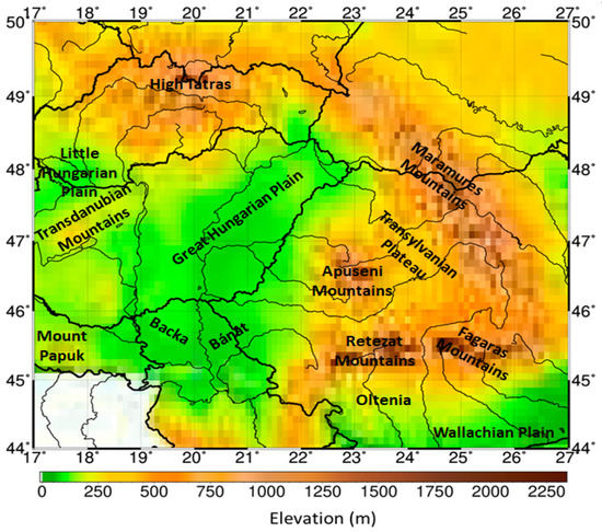
Figure 1.
The region studied. Geographical designations used in the study and the basic elevation data are also denoted.
4. Data
4.1. Climatic Data
The daily air temperature and wind speed data, together with geographical latitude data, are taken from the CarpatClim dataset [38,39,40]. The spatial resolution of the data is 0.1° × 0.1°, and the data refer to the period 1971–2000. The air temperature and wind speed data are homogenised data by using the MASH (Multiple Analysis of Series for Homogenization) technique, more precisely its latest version MASHv3.03 [41] without using metadata. Thirty-year monthly averages are obtained from daily values.
4.2. Human Data
The following human state variables are used: body mass (most important), body length, sex, and age. These data and the metabolic heat flux densities associated with activity levels (basal metabolism, walking, and the sum of the two) for two individuals are shown in Table 1.

Table 1.
Human state variables and metabolic heat flux densities of a man representing the average Hungarian man and a woman representing the average Hungarian woman.
The metabolic heat flux density of the 1st and 2nd persons is as close as possible to the metabolic heat flux density value of the average Hungarian man and woman [36], respectively.
5. Results
Four result types are presented and discussed: (1) some chosen results, which illustrate To–Ta point-clouds; (2) results characterising the relationship between M and BMI; (3) verification results; and (4) results characterising the human thermal load in the region depicted above.
5.1. Statistical Relationship between To and Ta
The To–Ta point-clouds, together with the regression lines for the months of July and January, as examples, are presented in Figure 2 and Figure 3, respectively. The statistical relationship is very strong in both cases. It is described by Equations (7) and (13).
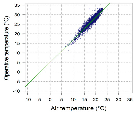
Figure 2.
Scatter chart of the operative temperature for the month of July as a function of air temperature for the CarpatClim dataset region in the period 1971–2000.
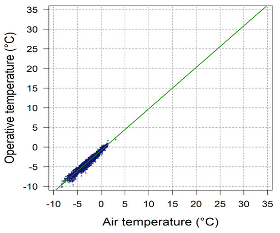
Figure 3.
Scatter chart of the operative temperature for the month of January as a function of air temperature for the CarpatClim dataset region in the period 1971–2000.
5.2. Interpersonal Variations of the Relationship between M and BMI
The scatter chart of total (basal plus walking) energy flux density as a function of BMI for all people in the Hungarian dataset together with persons 1 (black triangle) and 2 (black circle) [36] is presented in Figure 4. Red circles represent females, whilst blue triangles males. BMI values vary between 15 and 45 kgm−2, but the vast majority of points are located between 17 and 35 kgm−2. The BMI values of persons 1 and 2 are very close to 25 kgm−2, which is the median of BMI values. For the median value of BMI, M varies between 135 and 148 Wm−2, that is the interpersonal variability of M is roughly 10%. In all other cases, the interpersonal variability of M is less than 10%. Note that M increases linearly with increasing of BMI. The less M values are about 120 Wm−2, the largest ones can reach 180 Wm−2.
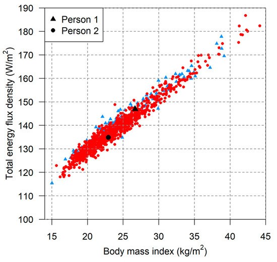
Figure 4.
Scatter chart of total energy flux density used during walking as a function of body mass index for the Hungarian human dataset. Blue: males, red: females.
5.3. Verification Results
Scatter plots between clothing thermal resistance values obtained calculating operative temperature on the basis of air temperature (statistical deterministic model) and by calculating operative temperature according to its definition (deterministic model, [19]) are presented in Figure 5. The results refer to the month of July and to the year for subjects 1 and 2. Subjects 1 and 2 are chosen since their total energy flux densities are as close as possible to the total energy flux densities of an average Hungarian male and female, respectively.
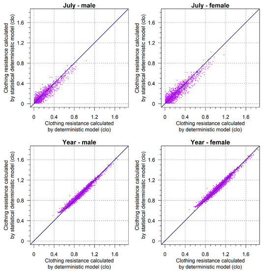
Figure 5.
Comparison of clothing thermal resistances obtained by calculating operative temperature by using statistical deterministic and deterministic procedures for persons 1 and 2 representing an average adult Hungarian male and female, respectively, in the month of July (top) and in the year (bottom) in the CarpatClim dataset region for the period 1971–2000. Each point-cloud contains about 6000 points. All figures, except Figure 3, are constructed by the R programming language [42].
Straight lines at 45 degrees are also plotted. The agreements presented are very good. The agreements for a year seem to be slightly better than those obtained for the month of July. The estimate obtained by the statistical-deterministic scheme for the month of July is slightly lower than the estimate obtained using the original scheme in the zones of higher rcl values (rcl is higher than 0.6 clo, such cases are obviously in the mountainous areas). Note that the male and female scatter plots are very similar.
The agreements are also presented in terms of spatial distribution for the month of July, separately for persons 1 and 2 in Figure 6 and Figure 7, respectively.
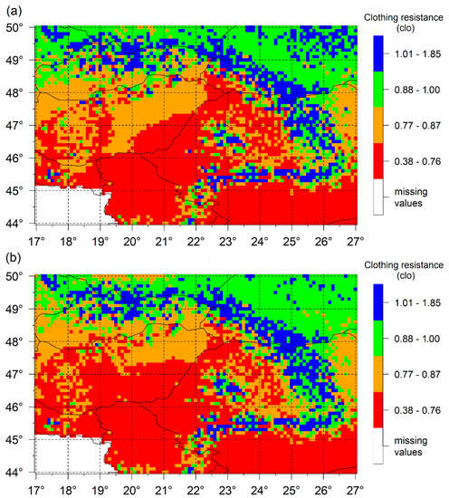
Figure 6.
Spatial distribution of clothing thermal resistance values for year obtained by calculating operative temperature by using deterministic (a) and by statistical deterministic (b) procedures for person 1 representing the average adult Hungarian male in the CarpatClim dataset region for the period 1971–2000.
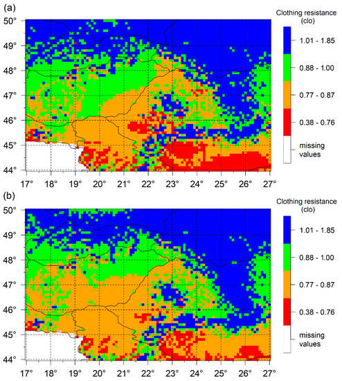
Figure 7.
Spatial distribution of clothing thermal resistance values for year obtained by calculating operative temperature by using deterministic (a) and by statistical deterministic (b) procedures for person 2 representing the average adult Hungarian female in the CarpatClim dataset region for the period 1971–2000.
5.4. Human Thermal Load
Human thermal load in terms of clothing thermal resistance will be separately analysed for the months of January and July and for the year.
5.4.1. January
The spatial distributions of clothing thermal resistance for persons 1 and 2 representing the average adult Hungarian male and female for the month January are presented in Figure 8.
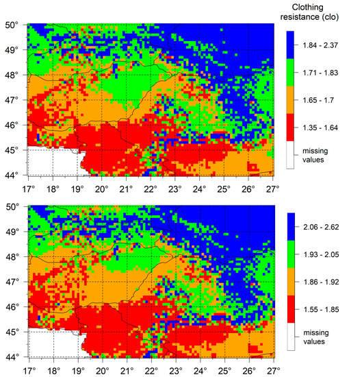
Figure 8.
Spatial distributions of January clothing thermal resistance values obtained by using the new statistical deterministic scheme for persons 1 and 2 representing the average adult Hungarian male (top) and female (bottom) in the CarpatClim dataset region for the period 1971–2000.
Note that the rcl ranges in the categories are non-linear. These are obtained using the main percentiles (0th, 25th, 50th, 75th, 100th) of the rcl values as category boundaries, we think this is an objective and reproducible categorisation method. Clothing thermal resistance values vary from 1.35 to 2.62 clo. The warmest areas are in Bačka, Banat, Oltenia, where the clothing thermal resistance values vary between 1.35–1.64 clo for person 1 and between 1.55 and 1.85 clo for person 2. The coldest areas (rcl values between 1.84 and 2.62 clo) may be found in mountain regions, such as the Retezat Mountains, Fagaras Mountains, Maramures Mountains, and in the north-eastern parts of the region. Areas with the largest thermal contrasts (large thermal load differences over small distances) are located in northern parts of Oltenia, i.e., on the southern slopes of the Carpathians. The largest rcl differences can reach 1 clo irrespective of which person is under consideration. Note that differences between the spatial structure of clothing thermal resistance fields representing the average adult Hungarian male and female are negligible; the greatest may be observed in the Great Hungarian Plain.
5.4.2. July
The same spatial distributions but for the month July are presented in Figure 9.
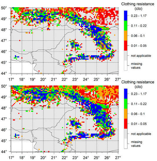
Figure 9.
Spatial distributions of July clothing thermal resistance values obtained by using the new statistical deterministic scheme for persons 1 and 2 representing the average adult Hungarian male (top) and female (bottom) in the CarpatClim dataset region for the period 1971–2000.
Note that clothing thermal resistance values for both persons vary between 0 and 1.2 clo. It can also be seen that the method is not applicable in the lowland and hilly regions of the Carpathian Basin. In such cases, the energy balance of the human body covered with clothing is not met because the model does not simulate the sweating process. Areas with the largest thermal contrast may be found on the southern slopes of the Retezat Mountains, the Fagaras Mountains, the Maramures Mountains, and very close to the location of the Iron Gates on the River Danube. In these areas, the largest rcl differences can reach 1 clo. Similarly to the month of January, the spatial distribution structures of the rcl maps of the average adult Hungarian male and female are very similar.
5.4.3. Year
The spatial distributions of annual clothing thermal resistance for the region and individuals considered are presented in Figure 6b and Figure 7b. As we can see, rcl values for both persons vary between 0.38 and 1.85 clo. Of course, the lowest rcl values are located in the southern (Bačka, Banat, Oltenia, Wallachian Plain) lowland areas of the region. The thermal load is somewhat greater (rcl values are between 0.77 and 1 clo) in the Great Hungarian Plain and the Transylvanian Plateau, and progressing towards the mountains rcl values become increasingly larger reaching maximum values of about 1.8 clo. Note that in the Podolian Upland (north-eastern part of the region) thermal load can be as large as in the mountains, such as in the Maramures Mountains, the High Tatras or Mount Papuk in the southern part of the region. Areas with the largest thermal contrast (rcl differences of about 1 clo over short distances) may be found in the southern parts of the region, for instance, at areas around Mount Papuk. As in the former cases, the spatial distribution structures of the rcl fields of persons 1 and 2 representing the average adult Hungarian male and female are quite similar. The greatest differences between them can be found in the areas of Podolian Upland.
6. Discussion
According to [27], those models may be used for climate classification purposes that: (1) are as simple as possible, (2) use as little as possible input data, (3) are physically well established, (4) define climate types simply and unequivocally, (5) treat both annual and seasonal characteristics, and (6) display the results transparently. Viewing all these points in turn, we will now examine the situation with our model. This model is a one-node model [29], metabolic heat flux density is simulated as simply as possible, only human body–air environment heat exchange processes are treated and there is no modelling of any thermoregulation processes, so the model is unable to simulate physiological processes on the basis of which the degree of the thermal stress could be estimated. So, the scheme is not suitable for estimating human thermal comfort issues [43], however, in our opinion it can be used for human thermal climate characterisation in terms of thermal load. In this paper, the issue of human thermal perception is not handled given the extreme subjectivity of the topic. We have also seen that the methodology is not applicable in warm climates, which is a clear disadvantage of the methodology. As regards point 2, the scheme uses less input data than the original scheme [19], using only air temperature and wind speed data as inputs. In connection with point 3, we can say that operative temperature is statistically evaluated via air temperature, although this reduces the physical basis of the model, the To–Ta statistical relationships are well correlated, therefore the scheme works well, at least in the Carpathian region. Climate types can be differentiated according to thermal load, which is expressed in terms of clothing thermal resistance values. In this study, different thermal load categories are not named. As regards point 5, the scheme is able to treat both the annual and the seasonal variations of clothing thermal resistance. In this study, we focused only on treating annual values, as well as the monthly values of the months of January and July. Lastly, there is no doubt that the transparent presentation of the results in the form of the maps is very important.
As regards human factors, it should be noted that the chosen persons representing average adult Hungarian male and female differ in their M values only 12 Wm−2. Despite small differences in M, differences in thermal load between the sexes were noticeable in some cases.
The spatial distribution results of clothing thermal resistance can be compared with the spatial distribution results of Physiologically Equivalent Temperature (P-E-T) obtained in [14]. In [14], the conditions and the tool used are as follows: the considered region is Hungary; CRU (Climatic Research Unit) data referring to the period 1961—1990 are used; among meteorological data air temperature, relative humidity, sunshine, cloudiness, and wind speed are taken as input data; the spatial resolution of meteorological data is 1 km × 1 km; some selected (not specified) surface morphological parameters are also used; the human data of the ‘standard human’ in P-E-T index are taken; and finally the P-E-T index calculation software together with the GIS (Geographical Information system) are applied as basic tools. Comparing our results of the month of January with the winter season results in [14], we can see two things: (a) both methodologies show cooling trend moving from southwest to northeast and (b) the spatial distribution of thermal load is orographically dependent. In the summer, the highest rcl values (about 1 clo) are in the mountains, where the lowest P-E-T values (about 15–16 °C) can be found. In contrast, in the lowland and hilly areas, where the rcl model is not applicable, the highest P-E-T values can reach 24 °C. For a more exact comparison, thermal perception results would be needed. This is a task for the future.
The results obtained can also be compared with the results obtained by generic methods. In this region, all three well known methods, the Köppen, Feddema and Holdridge methods were also used. According to Köppen [44], the heat availability in the region is mostly ‘warm temperate’ (symbol C), or ‘snow climate’ (symbol D). Köppen [28] defined the boundary between them analysing the territorial distribution and the heat demand of beeches and oaks as two typical climate marker plant species. According to our results, the ‘beech climate’, denoted as D, corresponds to annual rcl values of 1 clo and greater than 1 clo. The ‘oak climate’, denoted as C, represents a warmer climate, which is characterised by rcl values less than 1 clo. This agrees well with results obtained in [45]. We can see that in Köppen’s C climate rcl is between 0 and 0.8 clo. In Feddema climate classification method [46] thermal types are differentiated according to annual sums of potential evapotranspiration (PETa-sum). PETa-sum values are evenly distributed from 0 to maximum PETa-sum values, which may be higher than 1500 mm∙year−1. The thermal type categories used are ‘torrid’, ‘hot’, ‘warm’, ‘cool’, ‘cold’, and ‘frost’. Note that there is no intermediate thermal type category between ‘cool’ and ‘warm’, which seems to be reasonable from the point of view of human thermal climate classification. After [18], rcl values of mesomorphic human between 0.78 and 1.17 clo are obtained for PETa-sum values of 600 and 450 mm∙year−1, respectively. The main spatial distribution characteristics of annual human thermal load can also be recognised in the results obtained by the Holdridge method [47,48,49]. In lowland areas, where the rcl values are between 0.4 and 1 clo, the corresponding Holdridge life zone (HLZ) types are ‘cool temperate steppe’ and ‘cool temperate moist forest’. In Bačka and Banat, as the warmest (rcl values between 0.4 and 0.7 clo) area in the Carpathian Basin, the corresponding HLZ type is ‘warm temperate dry forest’. In the Carpathians, where the rcl values are above 1 and can reach 1.8 clo, the HLZ types ‘boreal wet forest’ and/or ‘boreal rain forest’ can be found. The mentioned HLZ types are obtained by using the CRU TS 1.2 database [50] and refer to the period 1971–2000 [48]. Note that the Holdridge method [47] is based on using potential evapotranspiration, just like the Feddema method [46].
The biggest shortcoming of the model is that it cannot be used in warm climates, but the concept of surface resistance that we have just applied to clothing can be extended to the unclothed skin surface in warm climates as well. In this case, one needs to estimate the evaporative resistance of the skin’s surface, which is changeable due to the sweating. Sweating is governed by thermal load: the greater the thermal load, the greater the sweating, and, conversely, the lower the thermal load, the less we sweat. Consequently, the evaporative resistance of the skin is high in the thermal perception category ‘neutral’, and conversely, it is very low (close to zero) in the thermal perception category ‘warm’ or ‘very warm’. This approach is also based on energy balance and is even more simple than the clothing resistance model. This model is currently being tested. Simplicity is an important requirement for the model to be suitable for use in everyday climate education and its simplicity also makes it possible to apply it to determine climate types. Going forward we would like to use a simple, easily applicable human-based climate classification method instead of the Köppen method.
7. Conclusions
A new clothing thermal resistance model is presented for climate classification purposes. Its main strengths are as follows: (1) only air temperature and wind speed data are used as meteorological inputs and (2) it is constructed for individual use, simulating the metabolic heat flux density of the walking human as simply as possible.
The following main conclusions can be drawn from the results obtained: (1) the annual rcl values in lowland and hilly areas are between 0.4 and 0.9 clo; (2) in the mountains, the highest rcl values can reach 1.8 clo; (3) the method is not applicable in the lowland and hilly areas of the region in the month of July; (4) thermal load differences between sexes are usually negligible, but in some places these differences are noticeable; (5) thermal load depends strongly on topography: rcl is roughly about 1 clo greater in mountains than in the lowlands; (6) the inter-season variations of rcl can reach 2 clo; and, finally, (7) the scheme can easily be adapted to any other region by determining new To–Ta relationships.
Author Contributions
Conceptualization, F.Á.; methodology, F.Á. and A.Z.; software, F.Á., A.Z. and H.B.; validation, F.Á., E.K., A.I.S. and Z.S.; formal analysis, F.Á., E.K., H.B. and Z.S.; investigation, F.Á., E.K., Z.S., A.I.S., H.B. and A.Z.; resources, A.Z.; data curation, F.Á., E.K. and A.Z.; writing—original draft preparation, F.Á.; writing—review and editing, F.Á. and Z.S.; visualization, E.K., H.B.; supervision, F.Á., E.K. and Z.S.; project administration, A.Z.; funding acquisition, A.Z. All authors have read and agreed to the published version of the manuscript.
Funding
This research received no external funding.
Informed Consent Statement
Not applicable.
Data Availability Statement
Informed consent was obtained from all subjects involved in the study.
Conflicts of Interest
The authors declare no conflict of interest.
References
- Yan, Y.Y. Climate comfort indices. In Encyclopedia of World Climatology; Oliver, J.E., Ed.; Springer: Dordrecht, The Netherlands, 2005; pp. 227–231. [Google Scholar]
- Epstein, Y.; Moran, D.S. Thermal comfort and heat stress indices. Indust. Health 2006, 44, 388–398. [Google Scholar] [CrossRef] [PubMed]
- de Freitas, C.R.; Grigorieva, E.A. A comprehensive catalogue and classification of human thermal climate indices. Int. J. Biometeorol. 2015, 59, 109–120. [Google Scholar] [CrossRef] [PubMed]
- Potchter, O.; Cohen, P.; Lin, T.P.; Matzarakis, A. Outdoor human thermal perception in various climates: A comprehensive review of approaches, methods and quantification. Sci. Total Environ. 2018, 631–632, 390–406. [Google Scholar] [CrossRef]
- Fanger, P.O. Thermal Comfort: Analysis and Applications in Environmental Engineering; Danmarks Tekniske Højskole, Danish Technical Press: Copenhagen, Denmark, 1970; p. 244. ISBN 8757103410/9788757103410. [Google Scholar]
- Fanger, P.O. Assessment of man’s thermal comfort in practice. Br. J. Ind. Med. 1973, 30, 313–324. [Google Scholar] [CrossRef]
- Becker, S. Bioclimatological rating of cities and resorts in South Africa according to the climate index. Int. J. Climatol. 2000, 20, 1403–1414. [Google Scholar] [CrossRef]
- Gagge, A.P.; Fobelts, A.P.; Berglund, L.G. A standard predictive index of human response to the thermal environment. ASHRAE Trans. 1986, 92, 709–731. [Google Scholar]
- Matzarakis, A.; Mayer, H. Heat stress in Greece. Int. J. Biometeorol. 1997, 41, 34–39. [Google Scholar] [CrossRef]
- Matzarakis, A.; Fröhlich, D.; Bermon, S.; Adami, P.E. Quantifying Thermal Stress for Sport Events—The Case of the Olympic Games 2020 in Tokyo. Atmosphere 2018, 9, 479. [Google Scholar] [CrossRef]
- Matzarakis, A.; Rutz, F.; Mayer, H. Modelling radiation fluxes in simple and complex environments—application of the RayMan model. Int. J. Biometeorol. 2007, 51, 323–334. [Google Scholar] [CrossRef]
- Matzarakis, A.; Graw, K. Human Bioclimate Analysis for the Paris Olympic Games. Atmosphere 2022, 13, 269. [Google Scholar] [CrossRef]
- Gulyás, Á.; Unger, J.; Matzarakis, A. Assessment of the microclimatic and thermal comfort conditions in a complex urban environment: Modelling and measurements. Build. Environ. 2006, 41, 1713–1722. [Google Scholar] [CrossRef]
- Gulyás, Á.; Matzarakis, A. Seasonal and spatial distribution of physiologically equivalent temperature (PET) index in Hungary. Időjárás 2009, 113, 221–231. [Google Scholar]
- Kántor, N.; Égerházi, L.; Unger, J. Subjective estimation of thermal environment in recreational urban spaces-Part 1: Investigations in Szeged, Hungary. Int. J. Biometeorol. 2012, 56, 1089–1101. [Google Scholar] [CrossRef]
- Bašarin, B.; Kržić, A.; Lazić, L.; Lukić, T.; Ðorđević, J.; Janićijević Petrović, B.; Čopić, S.; Matić, D.; Hrnjak, I.; Matzarakis, A. Evaluation of bioclimate conditions in two special nature reserves in Vojvodina (Nothern Serbia). Carpathian J. Earth. Environ. Sci. 2014, 9, 93–108. [Google Scholar]
- Bašarin, B.; Lukić, T.; Mesaros, M.; Pavić, D.; Ðorđević, J.; Matzarakis, A. Spatial and temporal analysis of extreme bioclimate conditions in Vojvodina, Nothern Serbia. Int. J. Climatol. 2018, 38, 142–157. [Google Scholar] [CrossRef]
- Ács, F.; Zsákai, A.; Kristóf, E.; Szabó, A.I.; Feddema, J.; Breuer, H. Clothing resistance and potential evapotranspiration as thermal climate indicators–The example of the Carpathian region. Int. J. Climatol. 2021, 41, 3107–3120. [Google Scholar] [CrossRef]
- Ács, F.; Zsákai, A.; Kristóf, E.; Szabó, A.I.; Breuer, H. Human thermal climate of the Carpathian Basin. Int. J. Climatol. 2021, 41, E1846–E1859. [Google Scholar] [CrossRef]
- Auliciems, A.; de Freitas, C.R. Cold Stress in Canada. A Human Climatic Classification. Int. J. Biometeorol. 1976, 20, 287–294. [Google Scholar] [CrossRef]
- de Freitas, C.R. Human Climates of Northern China. Atmos. Environ. 1979, 13, 71–77. [Google Scholar] [CrossRef]
- Yan, Y.Y.; Oliver, J.E. The Clo: A Utilitarian Unit to Measure Weather/Climate Comfort. Int. J. Climatol. 1996, 16, 1045–1056. [Google Scholar] [CrossRef]
- Yan, Y. Human Thermal Climates in China. Phys. Geogr. 2005, 26, 163–176. [Google Scholar] [CrossRef]
- Robaa, S.M.; Hasanean, H.M. Human Climates of Egypt. Int. J. Climatol. 2007, 27, 781–792. [Google Scholar] [CrossRef]
- Ács, F.; Kristóf, E.; Zsákai, A. New Clothing Resistance Scheme for Estimating Outdoor Environmental Thermal Load. Geogr. Pannonica 2019, 23, 245–255. [Google Scholar] [CrossRef] [Green Version]
- Ács, F.; Kristóf, E.; Zsákai, A.; Kelemen, B.; Szabó, Z.; Marques Vieira, L.A. Weather in the Hungarian Lowland from the Point of View of Humans. Atmosphere 2021, 12, 84. [Google Scholar] [CrossRef]
- Essenwanger, O.M. General Climatology 1C: Classification of Climates; Elsevier Science: Amsterdam, The Netherlands; New York, NY, USA, 2001; ISBN 978-0-444-88278-3. [Google Scholar]
- Köppen, W. Handbuch der Klimatologie. In Das Geographische System Der Klimate; Verlag von Gebrüder Borntraeger: Berlin, Germany, 1936; Volume I/C. [Google Scholar]
- Katić, K.; Li, R.; Zeiler, W. Thermophysiological Models and Their Applications: A Review. Build. Environ. 2016, 106, 286–300. [Google Scholar] [CrossRef]
- Weyand, P.G.; Smith, B.R.; Puyau, M.R.; Butte, N.F. The Mass-Specific Energy Cost of Human Walking Is Set by Stature. J. Exp. Biol. 2010, 213, 3972–3979. [Google Scholar] [CrossRef]
- Mifflin, M.D.; St Jeor, S.T.; Hill, L.A.; Scott, B.J.; Daugherty, S.A.; Koh, Y.O. A New Predictive Equation for Resting Energy Expenditure in Healthy Individuals. Am. J. Clin. Nutr. 1990, 51, 241–247. [Google Scholar] [CrossRef]
- Frankenfield, D.; Roth-Yousey, L.; Compher, C. Comparison of Predictive Equations for Resting Metabolic Rate in Healthy Nonobese and Obese Adults: A Systematic Review. J. Am. Diet. Assoc. 2005, 105, 775–789. [Google Scholar] [CrossRef]
- Dubois, D.; Dubois, E.F. The Measurement of the Surface Area of Man. Arch. Intern. Med. 1915, 15, 868–881. [Google Scholar] [CrossRef]
- Campbell, G.S.; Norman, J. An Introduction to Environmental Biophysics, 2nd ed.; Springer: New York, NY, USA, 1997; ISBN 978-0-387-94937-6. [Google Scholar]
- Auliciems, A.; Kalma, J.D. A Climatic Classification of Human Thermal Stress in Australia. J. Appl. Meteorol. 1979, 18, 616–626. [Google Scholar] [CrossRef]
- Zsákai, A.; Mascie-Taylor, N.; Bodzsar, E.B. Relationship between Some Indicators of Reproductive History, Body Fatness and the Menopausal Transition in Hungarian Women. J. Physiol. Anthropol. 2015, 34, 35. [Google Scholar] [CrossRef]
- Finn, K.J.; Saint-Maurice, P.F.; Karsai, I.; Ihász, F.; Csányi, T. Agreement Between Omron 306 and Biospace InBody 720 Bioelectrical Impedance Analyzers (BIA) in Children and Adolescents. Res. Q. Exerc. Sport 2015, 86, S58–S65. [Google Scholar] [CrossRef] [PubMed]
- Spinoni, J.; Antofie, T.; Barbosa, P.; Bihari, Z.; Lakatos, M.; Szalai, S.; Szentimrey, T.; Vogt, J. Comparing Four Drought Indicators in the Carpathian Region on a 0.1 × 0.1 Regular Grid for 1961–2010. In Proceedings of the 12th EMS–9th ECAC Conference, Lodz, Poland, 10–14 September 2012. [Google Scholar]
- Spinoni, J.; Szalai, S.; Szentimrey, T.; Lakatos, M.; Bihari, Z.; Nagy, A.; Németh, Á.; Kovács, T.; Mihic, D.; Dacic, M.; et al. Climate of the Carpathian Region in the Period 1961–2010: Climatologies and Trends of 10 Variables. Int. J. Climatol. 2015, 35, 1322–1341. [Google Scholar] [CrossRef] [Green Version]
- Cheval, S.; Birsan, M.-V.; Dumitrescu, A. Climate Variability in the Carpathian Mountains Region over 1961–2010. Glob. Planet. Chang. 2014, 118, 85–96. [Google Scholar] [CrossRef]
- Szentimrey, T. Multiple Analysis of Series for Homogenization; Hungarian Meteorological Service: Budapest, Hungary, 2011. [Google Scholar]
- R Core Team. R: A Language and Environment for Statistical Computing; R Foundation for Statistical Computing: Vienna, Austria, 2019. [Google Scholar]
- Staiger, H.; Laschewski, G.; Matzarakis, A. Selection of Appropriate Thermal Indices for Applications in Human Biometeorological Studies. Atmosphere 2019, 10, 18. [Google Scholar] [CrossRef]
- Kottek, M.; Grieser, J.; Beck, C.; Rudolf, B.; Rubel, F. World Map of the Köppen-Geiger Climate Classification Updated. Meteorol. Zeitschrift 2006, 15, 259–263. [Google Scholar] [CrossRef]
- Führer, E.; Horváth, L.; Jagodics, A.; Machon, A.; Szabados, I. Application of a New Aridity Index in Hungarian Forestry Practice. Időjaras 2011, 115, 205–216. [Google Scholar]
- Feddema, J.J. A Revised Thornthwaite-Type Global Climate Classification. Phys. Geogr. 2005, 26, 442–466. [Google Scholar] [CrossRef]
- Holdridge, L.R. Determination of World Plant Formations From Simple Climatic Data. Science 1947, 105, 367–368. [Google Scholar] [CrossRef] [PubMed]
- Ács, F.; Breuer, H. Biofizikai Éghajlat-Osztályozási Módszerek (Biophysical Climate Classification Methods); ELTE Reader: Budapest, Hungary, eBook; 2013; Available online: https://www.eltereader.hu/kiadvanyok/biofizikai-eghajlat-osztalyozasi-modszerek/ (accessed on 21 August 2022).
- Szelepcsényi, Z.; Breuer, H.; Kis, A.; Pongrácz, R.; Sümegi, P. Assessment of Projected Climate Change in the Carpathian Region Using the Holdridge Life Zone System. Theor. Appl. Climatol. 2018, 131, 593–610. [Google Scholar] [CrossRef]
- Mitchell, T.; Carter, T.; Jones, P.; Hulme, M. A Comprehensive Set of High-Resolution Grids of Monthly Climate for Europe and the Globe: The Observed Record (1901–2000) and 16 Scenarios (2001–2100). Tyndall Cent. Work. Pap. 2004, 55, 25. [Google Scholar]
Publisher’s Note: MDPI stays neutral with regard to jurisdictional claims in published maps and institutional affiliations. |
© 2022 by the authors. Licensee MDPI, Basel, Switzerland. This article is an open access article distributed under the terms and conditions of the Creative Commons Attribution (CC BY) license (https://creativecommons.org/licenses/by/4.0/).