Understanding Future Climate in the Upper Awash Basin (UASB) with Selected Climate Model Outputs under CMIP6

Abstract

Climate change makes the climate system of a given region unpredictable and increases the risk of water-related problems. GCMs (global climate models) help in understanding future climate conditions over a given region. In this study, 12 GCMs from the CMIP6 (coupled model intercomparison project six) were evaluated and ranked based on their abilities to describe the historical observed series. The ensemble mean of bias-adjusted best five models of average annual precipitation showed an increment with an uncertainty range of (2.0–11.9) and change in the mean of 6.4% for SSP2-4.5 and (6.1–16.1) 10.6% for SSP5-8.5 in 2040–2069 relative to the historical period. Similarly, for 2070–2099, increments of (2.2–15.0) 7.9% and (11.8–29.4) 19.7% were predicted for the two scenarios, respectively. The average annual maximum temperature series showed increments of (1.3–2.0) 1.6 °C for SSP2-4.5 and (1.7–2.3) 2.0 °C for SSP5-8.5 in 2040–2069. At the same time, increments of (1.7–2.3) 2.0 °C and (2.8–3.2) 3.0 °C were predicted for 2070–2099. Furthermore, it was predicted that the average annual minimum temperature series will have increments of (1.6–2.3) 2.0 °C and (2.2–2.9) 2.5 °C for 2040–2069 and (2.1–2.7) 2.4 °C and (3.7–4.2) 4.0 °C for 2070–2099 for the two scenarios, respectively. An increase in precipitation with increased land degradation in the sub-basin results in a higher risk of flood events in the future. Improved soil and water conservation practices may minimize the adverse impacts of future climate change on the loss of agricultural productivity.

1. Introduction

Securing water that satisfies every human need is the main priority and a challenge faced by many countries throughout the world. Socioeconomic growth, changing consumption patterns, and population growth are believed to be the main driving factors for the ever-increasing water demands [1]. The global freshwater composition that is accessible to humans is less than 1%, which makes it a limited resource [2]. In addition, the naturally uneven distribution of rainfall globally further adds to the complexity of making this resource accessible in adequate amounts to all.

Aside from the natural variation in rainfall distribution, in the past few decades, climate change has further contributed to this variability [3]. Anthropogenically-driven climate variability manifests itself via droughts and floods. Two recent events that support this point are the flood events that occurred in Mecca, Saudi Arabia, in April 2021 [4], and the drought event in southeastern Alaska, USA, in July 2019 [5].

According to a study by the NMA (National Meteorological Agency) on climate change adaptation, the major impacts of climate variability in Ethiopia are food insecurity, outbreaks of water-borne diseases, land degradation, and damage to infrastructure [6]. In particular, the Awash basin is a basin that supports a large population in several major cities and towns, including the capital city Addis Ababa [7]. The basin is highly utilized in the country in terms of water use (mainly for irrigation purposes). Most of the irrigation is practiced in the middle and lower parts of the basin. In addition, intensive rain-fed agriculture dominates the upper basin areas [8,9]. This part of the basin is mostly highland and is densely populated as compared to the middle and lower parts of the basin.

The Awash River is a major river that drains the Awash basin and a large proportion of its average annual flow comes from the upper basin areas. This is due to a relatively high average annual precipitation that falls on these parts of the basin [10]. In recent years, water security issues have become more evident. This is due to the occurrences of more frequent flood and drought events, especially in the middle and lower parts of the basin [11,12].

One of the widely used techniques in studying the impacts of climate change on the water resources of a given place is through the use of outputs from the Coupled Model Intercomparison Project of global climate models (CMIP-GCMs). CMIP-GCMs are mathematical equations that describe the global climate system with three-dimensional grids and are used to simulate the effects of greenhouse gas emissions on climate [13]. Since their introduction, the outputs from CMIP-GCMs have been essential in understanding the Earth’s past, present, and future climate. The use of CMIP-GCMs is often limited to global or regional scales mainly due to their coarse resolutions. However, with the proper application involving a combination of downscaling and bias correction techniques, CMIP-GCMs can be useful in understanding the local climate and play a vital role in the decision-making process for water resource planning and management [14,15].

In recent years, the challenge of predicting future climate has not only focused on climate modeling but also on how to use it. This is due to the sheer number of climate model outputs currently available worldwide. As a result, models often have to be evaluated for their performances in simulating the climate characteristics of the areas in which they are to be applied. The criteria to use for climate model evaluations depend on the climate model selection goals [16].

There are different versions and experiments of climate models generated at different institutions and locations throughout the world. This makes the inter-comparison between models highly cumbersome. This is the reason behind the establishment of the CMIP (climate model intercomparison project), i.e., to place the various model development efforts throughout the world (by different institutions) into one framework [17]. Currently, new sets of models belonging to the sixth CMIP framework have been released. The main differences between models released at each stage of the framework are mainly improvements in the model setups, resolutions, scenarios, and parametrization factors [18].

The CMIP6 archive currently holds model output results from more than 30 climate research centers found on different continents throughout the globe [17]. Each model is different; thus, the outputs generated for the same experiments and scenarios are different [19]. As a result, not all models perform well in certain locations. This is why there is a need to evaluate the capabilities of models and select those that have better performances in describing the local climate [16,20].

In practice, one climate model (or a small ensemble of climate models) is selected for climate change impact studies. In most cases, the selection could be based on a single criterion or a whole set of criteria. Climate models are often selected based on their skills to simulate the present and (near) past climate. This approach is known as the past performance approach. Another approach is called the envelop approach, where models covering a wide range of projections for one or more climate variables of interest are selected from the pool of available models [16,21].

To date, there is no clearly defined methodology to be used for evaluating and selecting a single or a group of climate models [16]. The selection method and process mainly depends on the aim of the study and the variables involved [16]. Most of the works to date have used statistical or data mining techniques. Moreover, there is a difference in the output (single or ensemble model), analysis period (daily, monthly, seasonal, and annual), and level (station, grid, regional, or spatially averaged).

The most common statistical techniques applied for the evaluation of climate models are performance indicators, descriptive statistics, and indices [22,23,24,25]. Data mining methods, such as singular value decomposition (SVD), principal component analysis (PCA), hierarchical clustering, symmetrical uncertainty (SU), and canonical correlation analysis (CCA) are also applied [20,21,26,27,28,29]. The main difference between these techniques is that data mining is a technique that is used to detect patterns and relationships in data, whereas statistical techniques are used to quantify data [30]. Using a combination of these various techniques instead of a single method helps to reduce the uncertainty of the wrong selection and improve it by including various characteristics of the time series. Techniques that are often used and help in incorporating multiple selection methods are skill score (SS) and multi-criteria decision analysis (MCDA) [16,31].

In the past, few attempts aimed to understand the climate of the Awash basin at large (and the upper Awash basin in particular). One of the earliest works on the Awash basin was by Hailemariam [32], where the outputs from three randomly selected CMIP3 GCMs (CCCM, GFD3, and GFDL) together with two scenarios were used in predicting a future runoff condition. After evaluating the potential of GCMs for their annual cycles, seasonal biases, variability, and trends, three CMIP5 GCMs were selected and used to study the impact of climate change by Taye et al. [33]. The impact of climate change on the river basin was studied with help of a few selected models from the CMIP5 archive for different scenarios identified from previous works [34]. Similarly, an ensemble of two GCMs [35] and three selected GCMs [36] from the CMIP5 archive was used to characterize the river flow in the first case and to estimate the river nutrient load in the second one. The ensemble mean of five randomly selected GCMs from the CMIP5 archive was used in characterizing the hydrometeorological situation for the upper Awash basin by Emiru et al. [37]. Most recently, similar research that was published also suggested a group of four climate models, which came from different ensembles of the CMIP6 as an output [38]. Two approaches that combined envelop and past performance approaches were put to use in evaluating the outputs of CMIP6 after [16].

Previous climate change projection efforts in the Awash or upper Awash sub-basin focused on putting into use a few randomly selected climate models without thoroughly evaluating their capability to simulate the climate system over UASB. Therefore, the novelty of this study was through addressing this shortcoming through the execution of more robust evaluation criteria that mainly relied on the application of statistical and data mining techniques. The main outcome of this study will be in identifying a model/s that has an overall good performance over the sub-basin. In addition, a prediction of future climate conditions with the newly selected model will be performed later and compared with similar earlier findings in the sub-basin.

2. Materials and Methods

2.1. Study Area and Data Used

The study focused on the upper Awash sub-basin, which is found in central Ethiopia (Figure 1), with a longitude of 37${}^{°}$57${}^{\prime }$4${}^{″}$ E–39${}^{°}$17${}^{\prime }$28${}^{″}$ E and a latitude of 8${}^{°}$4${}^{\prime }$52${}^{″}$ N–9${}^{°}$19${}^{\prime }$47${}^{″}$ N. The basin has a total drainage area of 12,043 km${}^2$ and contributes the majority of the annual flow to the larger Awash basin. The mean annual precipitation ranges from 861 to 1223 mm at Boneya and Addis Ababa, respectively. The mean annual temperature is in the range of 17 °C at Addis Ababa and 21 °C in Melkasa. The topography of the drainage basin ranges from 3561 m in altitude near ArbGebya and as low as 1547 m at Koka lake.

For the climate model evaluation, a total of 15 rainfall and 10 temperature stations were used. The stations used are shown in

Table 1. List of names of meteorological stations in the upper Awash sub-basin with their locations (UTM (Universal Transverse Mercator)) and altitude (m) were used for the analysis.

No.	Station Name	Location (y)	Location (x)	Altitude
1	Addis Ababa Obs *	472,248.08	996,952.4	2386
2	Addis Alem **	432,225.93	999,552.91	2372
3	Aleltu	516,771.63	1,016,119.33	2648
4	Ambo **	372,449.79	993,358.73	2068
5	Asgori *	426,775.97	971,700.31	2072
6	Boneya	460,591.24	971,046.06	2251
7	Bui **	450,940.01	920,899.89	2054
8	ChefeDonsa	513,542.53	991,537.73	2392
9	Debrezeit *	494,500.33	965,370.79	1900
10	Ejere	528,246.66	969,798.67	2254
11	Enselale	435,870.79	987,532.37	2000
12	Ginchi	404,738.43	996,808.09	2132
13	Hombole	475,209.16	925,006.74	1743
14	Huruta *	537,697.21	900,012.17	2044
15	Melkasa *	534,861.76	928,532.98	1540
16	Mojo	511,901.68	951,220.7	1763
17	Nazret	531,179.91	945,113.49	1622
18	Sebeta	459,322.66	986,027.98	2220
19	Teji	430,354.91	976,481.48	2091
20	Tulu Bolo *	414,188.26	958,456.67	2100
21	Welenchiti	547,305.49	958,395.38	1458
22	Woliso **	388,113.76	945,249.62	2058

N.B: The ones without and with a single star (*) are used for precipitation and the others with one star (*) and a double star (**) are used to differentiate stations used for temperature analysis.

.

Overall, 12 climate models were preliminarily identified from the WCRP CMIP6 archive (https://esgf-node.llnl.gov/search/cmip6/ (accessed on 17 August 2021)) to be used for the study based on model availability for all variables (precipitation, Tmax, and Tmin) for the historical time period. The criteria used to filter the models were daily data, 100 km nominal resolution, and source type: AOGCM and from the r1i1p1f1 variant. The models were accessed from this site on 17 August 2021. The list of models used for analysis is shown in

Table 2. List of climate models used in the selection process.

Model	Institute	Country
MRI-ESM2-0	Meteorological Research Institute	Japan
ECEARTH3-CC	EC-Earth consortium	Sweden
NorESM2-MM	Norwegian Climate Center	Norway
TaiESM1	Academia Sinica	Taiwan
ECEARTH3.Veg	EC-Earth consortium	Sweden
MPI-ESM1.2.HR	Max Planck Institute for Meteorology	Germany
ECEARTH3	EC-Earth consortium	Sweden
CMCC-ESM2	Centro Euro-Mediterraneo sui Cambiamenti Climatici	Italy
GFDL-CM4	NOAA	USA
GFDL-ESM4	NOAA	USA
INM-CM4-8	Institute for Numerical Mathematics	Russia
INM-CM5-0	Institute for Numerical Mathematics	Russia

.

2.2. Methodology

2.2.1. Climate Model Selection

The process begins with extracting the outputs of GCMs for the given station and time period with the help of the CDO (climate data operator) [39]. GCM outputs were extracted to each climate station using the inverse distance weighting (IDW) interpolation technique under CDO. The comparison between the outputs of GCMs and observed data is based on spatially averaged values for the sub-basin. For spatial averaging of station point data, the Thiessen polygon technique was applied. All historical climate series were bias adjusted using the corresponding observed series at each station.

The intentions of the methodologies applied here mainly depend on displaying the important characters of the climate time series that play a critical role in climate impact studies. Thus, based on the intensive literature review conducted on the current methodologies and the objective of this paper, a combination of methodologies was used. The selection or evaluation was based on historical/observed data and was performed at four-time scales or levels—monthly, seasonal (JJAS and MAM), and annual. The two seasons were selected because they are important rainy seasons that determine annual water availability in the sub-basin. It is assumed that the analysis of these time scales will help researchers grasp all statistical characteristics of the time series.

In total, six methodologies were applied, which highlight the various characteristics of the time series. The first technique attempts to fit probability distributions to all climatic variables and checks which climatic models have similar distributions to the observed climate variable. This was performed using the gamlss package [40] under R programming software [41]. The result of the distribution analysis was evaluated between the observed and climate model series using the Akaike information criterion (AIC). Then the climate model or models that have similar distribution(s) is/are assumed to be the model(s) that is/are capable of better describing the observed series.

The second technique observes the trend using the Mann–Kendall (MK) test [42,43]. In detecting the trend, the MK test calculates statistic ‘S’ by ranking the data and calculating the sign as described in Equation (1) [42].

$$S=\sum _{i=1}^{n-1}\sum _{j=i+1}^{n}sgn(x_j-x_i)$$

(1)

where x_j are the data ranked from i = 1, 2, 3, …, n−1, and x_i are the data ranked from j = i + 1, 2, …, n

The sign is the difference between the original data x_i, shortened by one data point, and the data itself without the first data point x_j.

$$sgn(x_j-x_i)=\left\{\begin{array}{c}+1if(x_j-x_i)>0\hfill \\ 0if(x_j-x_i)=0\hfill \\ -1if(x_j-x_i)<0\hfill \end{array}\right.$$

(2)

It is observed that when the data point (observation) is more (n ≥ 10), statistic ‘S’ becomes normally distributed with the mean (E(S)) equal to zero and variance calculated as follows:

$$Var\left(S\right)=\frac{n(n-1)(2n+5)-{\sum }_{t=1}^m{t}_1(t_1-1)(2t_1+5)}{18}$$

(3)

where n is the number of data points and $t_i$ are the ties of the sample data series. The test statistic ($Z_c$) is calculated as:

$$Z_c=\left\{\begin{array}{c}\frac{S-1}{\sigma }ifS>0\hfill \\ 0ifS=0\hfill \\ \frac{S+1}{\sigma }ifS<0\hfill \end{array}\right.$$

(4)

where $\sigma$ is the standard deviation of the statistic ‘S’. From this test statistic, (Z_c) was concluded, a positive value indicates an upward trend, and a negative value is the contrary. According to [43], this approach works well for data where there is no significant correlation at lag 1, if there is a significant correlation at lag 1, the modified MK test is applied. The method calculates the significance of the trend by modifying the variance of the MK test statistic (‘S’) by the ESS (effective sample size). The significance is determined based on the p-value at a significance level of 0.05. Therefore, if the p-value is greater than 0.05, then we accept the null hypothesis that there is no significant trend in the data, and if it is less than or equal, the reverse is true. The results of the MK test can further be supported by Sen’s slope method [44], which calculates the magnitude of the trend (slope ($T_i$)) as shown in Equation (5) below:

$$T_i=\frac{X_j-X_i}{j-i}$$

(5)

The median of the N value of $T_i$ represents Sen’s slope estimator, which is calculated as follows;

If N appears to be odd:

$$Q_{med}=T\frac{(N+1)}{2}$$

(6)

If N is even, then:

$$Q_{med}=\frac{(T_{\frac{N}{2}}+T_{\frac{(N+2)}{2}})}{2}$$

(7)

Here, a positive $Q_{med}$ value in the time series indicates an upward trend and a negative value the reverse.

In the third approach, four performance metrics were applied to identify which climate model/s better simulated the observed series. The selected measures were coefficient of determination ($R^2$), root mean squared error (RMSE), mean absolute error (MAE), and BIAS. The performance measures were each applied for all time steps. Moreover, a rank was assigned to each model based on the magnitude of the performance measure. Models that had overall good performances at all four-time steps were identified by summing the ranks at the corresponding time steps and ranking again.

Another technique applied a time series clustering technique to identify which climate model could capture the stochastic process of the observed series much better. For this, the integrated periodogram algorithm developed by [45] was used in the TSclust package [46] under R. This data mining approach attempts to group time series into clusters based on the integrated periodogram ($d_{IP}$) as a distance (dissimilarity) measure. The periodogram technique helps with setting the comparison to be in the frequency domain and this enables characterizing each time series in terms of its underlying stochastic behavior. The dissimilarity measure was calculated using Equation (8) [45],

$$d_{IP}(X_T,Y_T)={\int }_{-\pi }^{\pi }|F_{X_T}\left(\lambda \right)-F_{Y_T}\left(\lambda \right)|d\lambda$$

(8)

where the normalized cumulative periodograms at each data point j are given by:

$$F_{X_T}\left({\lambda }_j\right)=\frac{1}{C_{X_T}}\sum _{i=1}^j{I}_{X_T}\left({\lambda }_i\right)$$

(9)

$$F_{Y_T}\left({\lambda }_j\right)=\frac{1}{C_{Y_T}}\sum _{i=1}^j{I}_{Y_T}\left({\lambda }_i\right)$$

(10)

The weights used for normalizing the periodograms are as shown below, where m is the number of data points in the original data series:

$$C_{X_T}=\sum _{i=1}^m{I}_{X_T}\left({\lambda }_i\right)$$

(11)

$$C_{Y_T}=\sum _{i=1}^m{I}_{Y_T}\left({\lambda }_i\right)$$

(12)

The periodograms calculated at each time stamp (k) of the observed series are given by:

$$I_{X_T}\left({\lambda }_k\right)=\frac{1}{T}{|\sum _{t=1}^T{X}_t{e}^{-i{\lambda }_{k}t}|}^2$$

(13)

$$I_{Y_T}\left({\lambda }_k\right)=\frac{1}{T}{|\sum _{t=1}^T{Y}_t{e}^{-i{\lambda }_{k}t}|}^2$$

(14)

Here, ${\lambda }_K=\frac{2\pi k}{T}$ is the frequency component corresponding to the input data sequence k ($k=1,2,...,n$); $n=\frac{T-1}{2}$ depends on the total data length of the observed series (T). In addition, $X_t$ and $Y_t$ correspond to each pair of time series for which the dissimilarity measure is to be calculated. Moreover, the term i in Equations (13) and (14) indicates the imaginary term from the Fourier transform of each pair of series.

A pairwise matrix of dissimilarity measure can be produced from the above procedure at which clustering is performed using the agglomerative hierarchical clustering technique under TSclust package in R that applies the hclust() function from the stats package. The classification into a cluster group or merge between clusters is through complete linkage criteria [45].

The fifth technique used is principal component analysis (PCA), which is a dimensionality reduction technique that transforms a large number of correlated variables into much smaller uncorrelated variables called principal components (PCs) [47]. Here, the 11 variables (1 observed + 10 climate models) were displayed into two-dimensional axes called principal components (PCs). The original data points for each variable can be plotted into a two-dimensional space called a score plot. This is done by projecting all data points into those two PCs using the loading vectors obtained from the covariance matrix. The score plot indicates that points closer to the origin are closer to average, points near to each other are similar, and points further outward are outliers. The correlation between each variable can be better viewed using a loading plot. This plot is obtained by plotting the eigenvectors and indicates the contribution of each loading to the PC. The relative length of the vector indicates its contribution to each PC and the angle between the vectors indicates the similarity between the variables. That means that if the angles between the two adjacent loading vectors of variables are smaller, they are more correlated, if orthogonal, they are not related, it they are in the reverse direction, then they are negatively correlated. A combined plot of the score and loading plot is known as a biplot [48].

In the end, the spatial performances of the models were evaluated via correlation analyses and the RMSE as model fit criteria. The two techniques were applied at the station level and later interpreted using a rank-based methodology.

2.2.2. Downscaling, Bias Adjustment, and Future Scenarios

The outputs of GCMs have to be downscaled and bias-adjusted before applying them to real-world situations. This is mainly because the outputs of climate models have biases due to imperfect conceptualization and parametrization, insufficient length of data records, quality of reference data sets, and insufficient spatial resolution [49,50]. Therefore, often the downscaling of GCM outputs is performed by applying either dynamical or statistical downscaling approaches. Dynamic downscaling produces RCMs, which are at finer scales (<50 Km) using GCM boundary conditions and are computationally expensive procedures [51]. More often, statistical downscaling is preferred compared to the former one since there is no drawback (because of the high computational requirements and the ability to bias-adjust). Here, the bias adjustment was performed by creating a statistical link between the large-scale predictors and a finer-scale predictor.

Furthermore, statistical downscaling approaches can be classified into two types—perfect prognosis (PP) and model output statistics (MOS) [52]. PP methods work by creating day-to-day statistical relationships between large-scale predictors and local-scale predictors during the calibration phase. Moreover, the calibrated statistical relationship will be used later for downscaling a predictor variable. Examples of PP could be regression, weather generators, and analog methods. In MOS, there is no day-to-day correspondence, rather, a statistical transfer function is applied during the calibration phase and later used for the downscaling operation [53]. Additive correction/scaling, variance correction, and quantile mapping are some of the techniques under MOS.

Here, both the precipitation and temperature stations were first downscaled to each ground station shown in Table 1 using the IDW technique (15) and later bias-corrected using the quantile matching (QM) approach.

$$V_{St.}=\frac{(\frac{V_{G{P}_1}}{D_1}+\frac{V_{G{P}_2}}{D_2}+\frac{V_{G{P}_3}}{D_3}+\frac{V_{G{P}_4}}{D_4})}{{\sum }_{i=1}^4\frac{1}{D_i}}$$

(15)

where $V_{St.}$ is the variable at the station level, $V_{G{P}_i}$ is the variable at the grid point level, and $D_i$ is the distance from the grid point to the specific station.

The QM method uses empirical CDF obtained from the actual observations and requires no assumption of the underlying distribution; it was applied here to the climate model with a top rank [54]. The bias adjustments in this study were performed under R with the help of the qmap package [50] on the daily climate series. The theoretical assumption of QM was to adjust the bias and is shown in Equation (16) as follows:

$$x_f=F_f^{-1}\left(F_o\left(x\right)\right)$$

(16)

where: $x_f$ is the value of the bias-adjusted future climate variable; $F_o\left(x\right)$ is the ECDF of the observed variable; $F_f^{-1}$ is the inverse ECDF of the future GCM; and x is the value of the future GCM variable before the bias adjustment.

Three future scenarios (SSP1-2.6, SSP2-4.5, and SSP5-8.5) and three time periods (near-century (2022–2039), mid-century (2040–2069), and end of the century (2070–2099)) were used to understand the future climate of the upper Awash basin. The three scenarios each consider sustainable, middle, and worst future socioeconomic conditions. The worst-case scenario is the upper boundary in terms of the range of scenarios available and it can be considered an update of RCP8.5 of CMIP5. The second one, which is SSP2-4.5, indicates the medium pathway for the future increase in greenhouse gas emissions, which is similar to the RCP4.5 of CMIP5.

In addition, uncertainty limits were added to the calculated expected mean changes (for precipitation $({\overline{x}}_{predicted}-{\overline{x}}_{observed})/\left({\overline{x}}_{observed}\right)$ and the Temp $({\overline{x}}_{predicted}-{\overline{x}}_{observed})$) of the mean annuals by using the standard deviation across each series (predicted and observed). For example, for the predicted series, the limits were $={\overline{x}}_{predicted}\pm x_{standarddeviation,predicted}$. The same technique was applied when calculating the limits of the observed.

3. Results

3.1. Selection of Climate Model

All the methods used were selected to highlight the very important characteristics of a climate time series, which could play a critical role in addressing the future climate impact in the study area. The evaluation criteria were distribution fitting, trend analysis, performance measures, DTW-based hierarchical clustering, PCA analysis, spatial correlation, and RMSE (root mean squared error). A total of twelve climate models as shown in Table 2 were identified initially based on the common availability of climate models for the three climatic variables (precipitation, maximum temperature, and minimum temperature). The models were evaluated for their statistical characteristics based on seven different evaluation criteria and different time levels (monthly, monthly average, seasonal, and annual). The monthly series was obtained by summing/averaging precipitation/temperature daily series in each month. The monthly average was conducted by taking those monthly values and further averaging them across the total period of analysis for each month.

3.1.1. Identification of Distribution

For the observed and climate model series, the best possible distributions were identified with the help of gamlss package in R [40]. For example, for the precipitation data of the monthly average, JJAS, MAM, and annual series, the observed data were found to have normal (NO), logistic (LO), gamma (GA), and normal (NO) distributions, respectively. The definitions for each distribution type used in fitting the three climate variables are given in Appendix A. The PDF and CDF plots for only the monthly average precipitation series of the observed and climate models are shown in Figure 2 below.

The results of the distribution analysis for all three climatic variables and different time steps of the analysis of both the observed and climate model series are summarized in

Table 3. Fitted distributions for all three climatic variables across the four time steps of both the observed and climate model series.

	Monthly Average		JJAS		MAM		Annual
Data Type	AIC	DT	AIC	DT	AIC	DT	AIC	DT
Precipitation
Observed	221.62	NO	359.84	LO	348.147	GA	370.72	NO
CMCC-ESM2	210.09	SN2	229.72	SN2	272.3	SEP1	359.19	SN2
ECEARTH3	213.9	SN2	268.16	WEI	277.63	WEI3	362.99	SN2
ECEARTH3-CC	229.69	RG	257.03	GA	285.2	GA	378.79	RG
ECEARTH3-Veg	228.64	SEP1	249.17	SEP3	274.55	RG	381.82	IGAMMA
GFDL-CM4	196.06	WEI3	254.98	WEI	266.21	NO	345.16	WEI
GFDL-ESM4	214.78	SEP3	233.74	SEP2	259.64	NO	364.56	IGAMMA
MPI-ESM1-2-HR	217.1	SEP1	263.67	WEI3	275.74	SEP1	366.19	SEP1
MRI-ESM2	232.6	NO	261.15	LO	271.72	GA	381.7	NO
NorESM2-MM	229.68	LO	277.26	LO	295.01	GA	378.77	LO
TaiESM1	209.12	NO	237.44	IGAMMA	272.38	LO	358.22	NO
INM-CM4-8	233.88	WEI	281.42	SEP2	238.5	WEI3	382.97	WEI3
INM-CM5-0	226.62	SN2	280.22	NO	261.28	WEI2	377.17	SN2
Maximum Temperature
Observed	45.97	SN2	28.93	RG	51.31	WEI	13.19	PE2
CMCC-ESM2	32.12	WEI3	52.57	SN2	37.6	LO	32.12	WEI3
ECEARTH3	30.55	NO	44.69	WEI3	53.16	GT	30.55	NO
ECEARTH3-CC	30.06	SN2	39.55	GG	42.85	SN2	30.06	SN2
ECEARTH3-Veg	26.53	NO	42.93	SN2	45.23	NO	26.53	NO
GFDL-CM4	8.59	SN2	37.81	RG	45.1	IGAMMA	8.59	SN2
GFDL-ESM4	27.57	SN2	42.36	WEI3	49.34	LO	27.57	SN2
MPI-ESM1-2-HR	14.35	NO	34.3	SN2	57.13	NO	14.35	NO
MRI-ESM2	10.66	NO	42.33	WEI	42.31	PE2	10.66	NO
NorESM2-MM	37.52	SHASH	58.02	SN2	55.42	WEI3	37.52	SHASH
TaiESM1	2.78	WEI3	31.94	WEI	25.06	NET	2.78	WEI3
INM-CM4-8	14.07	WEI3	14.57	IGAMMA	31.78	PE	14.07	WEI3
INM-CM5-0	11.02	WEI	27.42	LO	35.8	NET	11.02	WEI
Minimum Temperature
Observed	42.35	SEP1	30.9	NO	34.09	NO	16.98	IGAMMA
CMCC-ESM2	33.67	SEP1	24.05	SN2	45.87	GA	33.67	SEP1
ECEARTH3	44.68	WEI3	47.64	WEI	23.2	NET	44.68	WEI3
ECEARTH3-CC	40.14	SN2	52.83	WEI	31.7	GU	40.14	SN2
ECEARTH3-Veg	45.88	WEI3	16.64	BCPEo	28.47	PE	45.88	WEI3
GFDL-CM4	3.73	IGAMMA	-6.15	RG	28.03	IGAMMA	3.73	IGAMMA
GFDL-ESM4	31	WEI	15.08	WEI3	38.77	NO	31	WEI
MPI-ESM1-2-HR	21.35	IGAMMA	10.89	SEP3	3.36	NO	21.35	IGAMMA
MRI-ESM2	29.13	RG	9.45	GT	30.08	RG	29.13	RG
NorESM2-MM	50	SHASH	37.67	SEP1	45.7	WEI	50	SHASH
TaiESM1	16.68	NET	12.72	LO	34.01	LO	16.68	NET
INM-CM4-8	16.43	WEI	-6.83	WEI	33.46	SN2	16.43	WEI
INM-CM5-0	12.78	SEP3	-7.68	SN2	40	IG	12.78	SEP3

NB: highlighted in grey are models that shared the same distribution as the observed time series across each time period of the analysis. DT = distribution type.

. For the precipitation series, it can be deduced that the MRI-ESM2-0 model was capable of having similar distributions with the observed series at all time steps. Moreover, TaiESM1 had similar distributions at the monthly average and annual time steps. NorESM2-MM had similar distributions only at seasonal time steps and ECEARTH3-CC only at MAM.

Regarding the maximum temperature series, none of the climate models showed consistent similarities across different time steps, as shown in Table 3. Here, three models had similar distribution types at monthly average time steps. The GFDL-CM4 model had the same distributions with the observed series twice across those four time steps. Moreover, none of the models had similar distributions at the annual level. Few models shared a similar distribution type with the observed series in the case of minimum temperature. Here, similar distributions were observed only for model CMCC-ESM2 at the monthly average, and MPI-ESM1-2-HR and GFDL-ESM4 at the MAM time steps, respectively. There were no models that were capable of having similar distributions at the annual time step, as shown in Table 3 below.

3.1.2. Trend Analysis

The trend analysis was performed similarly at four different levels (the same as in the distribution analysis). The precipitation series indicates that almost all of the models had similar trends to the observed series across all time steps. The exceptions are ECEARTH3 and ECEARTH3-CC at JJAS and INM-CM4-8 at the monthly average and annual time level, as shown in

Table 4. Results of the trend analysis for all three climatic variables across the four time steps for the observed and climate model series.

Data Type	Annual		Monthly Ave.		JJAS		MAM
	Z-val	Sen S.	Z-val	Sen S.	Z-val	Sen S.	Z-val	Sen S.
Precipitation
Observed	−0.43	−0.91	−0.43	−0.08	−0.07	−0.06	0.07	0.05
CMCC-ESM2	0.04	0.09	0.04	0.01	−1.39	−0.32	1.82	0.89
ECEARTH3	1.39	3.62	1.39	0.30	2.64	1.06	−0.21	−0.05
ECEARTH3-CC	1.78	5.61	1.78	0.47	3.14	1.00	−0.39	−0.29
ECEARTH3-Veg	0.39	1.51	0.39	0.13	0.64	0.21	−0.36	−0.27
GFDL-CM4	1.68	3.14	1.68	0.26	1.04	0.33	−0.18	−0.05
GFDL-ESM4	−0.25	−1.02	−0.25	−0.09	−1.43	−0.25	−0.86	−0.45
MPI-ESM1-2-HR	0.21	0.55	0.21	0.05	−0.25	−0.08	0.61	0.17
MRI-ESM2	1.57	4.52	1.57	0.38	0.5	0.25	0.46	0.31
NorESM2-MM	1.21	3.29	1.21	0.27	0.14	0.1	0.14	0.08
TaiESM1	−0.86	−1.94	−0.86	−0.16	−1.61	−0.5	0.64	0.24
INM-CM4-8	2.87	4.25	2.87	0.35	1.32	1.04	1.04	0.29
INM-CM5-0	0.71	2.71	0.71	0.23	0.00	−0.01	1.14	0.52
Maximum Temperature
Observed	7.36	0.03	7.36	0.03	1.27	0.02	2.38	0.05
CMCC-ESM2	2.13	0.02	2.13	0.02	1.00	0.03	0.34	0.01
ECEARTH3	4.32	0.04	4.32	0.04	2.54	0.05	1.8	0.05
ECEARTH3-CC	1.29	0.01	1.29	0.01	3.23	0.03	1.00	0.02
ECEARTH3-Veg	3.4	0.03	3.4	0.03	2.97	0.04	0.37	0.01
GFDL-CM4	1.32	0.02	1.32	0.02	0.4	0.01	0.79	0.02
GFDL-ESM4	2.48	0.02	2.48	0.02	0.32	0.01	2.38	0.05
MPI-ESM1-2-HR	0.08	0.00	0.08	0.00	0.26	0.01	0.00	0.00
MRI-ESM2	0.00	0.00	0.00	0.00	0.69	0.02	−1.47	−0.01
NorESM2-MM	1.99	0.02	1.99	0.02	0.26	0.01	0.63	0.01
TaiESM1	6.63	0.02	6.63	0.02	1.95	0.03	1.69	0.02
INM-CM4-8	2.48	0.03	2.48	0.03	2.85	0.04	1.74	0.02
INM-CM5-0	2.99	0.02	2.99	0.02	1.56	0.02	1.48	0.02
Minimum Temperature
Observed	1.8	0.02	1.8	0.02	2.32	0.03	1.11	0.02
CMCC-ESM2	1.57	0.02	1.57	0.02	2.37	0.02	0.64	0.01
ECEARTH3	2.8	0.06	2.8	0.06	3.38	0.07	3.01	0.03
ECEARTH3-CC	1.41	0.03	1.41	0.03	4.02	0.05	1.69	0.03
ECEARTH3-Veg	4.02	0.04	4.02	0.04	2.64	0.05	1.89	0.01
GFDL-CM4	1.22	0.01	1.22	0.01	2.48	0.02	−0.79	−0.01
GFDL-ESM4	4.76	0.04	4.76	0.04	4.13	0.02	2.46	0.04
MPI-ESM1-2-HR	1.00	0.01	1.00	0.01	0.79	0.01	−0.87	−0.01
MRI-ESM2	5.9	0.04	5.9	0.04	5.58	0.04	2.09	0.03
NorESM2-MM	0.87	0.01	0.87	0.01	1.76	0.02	0.48	0.02
TaiESM1	0.79	0.01	0.79	0.01	6.24	0.02	1.69	0.02
INM-CM4-8	8.95	0.02	8.95	0.02	6.83	0.02	1.06	0.01
INM-CM5-0	2.38	0.02	2.38	0.02	3.73	0.01	2.01	0.03

NB: the ones shaded in gray show that the models have similar trend test outcomes, i.e, if both the observed and the model are significant/insignificant, then the z-values are highlighted.

. Even though there was no significant trend, the Sen slope values of model TaiESM1 indicated the same trend direction as observed in the series but with different magnitudes.

For the maximum temperature series, ECEARTH3-CC did not have a similar trend to the observed series at any of the time steps. Four models (CMCC-ESM2, NorESM2-MM, TaiESM1, and INM-CM5-0) had similar trends at three-time steps out of four. Moreover, GFDL-ESM4 was the only model that had similar trend characteristics as the observed series at all time steps, as shown in Table 4.

Furthermore, among the ten models, CMCC-ESM2, ECEARTH3-CC, GFDL-CM4, and TaiESM1 had similar trends to the observed minimum temperature series across all time steps, whereas models ECEARTH3, GFDL-ESM4, MRI-ESM2-0, and INM-CM5-0 had the least. Two models, MPI-ESM1-2-HR and NorESM2-MM, showed similarities at all time steps except for the JJAS season, as shown in Table 4.

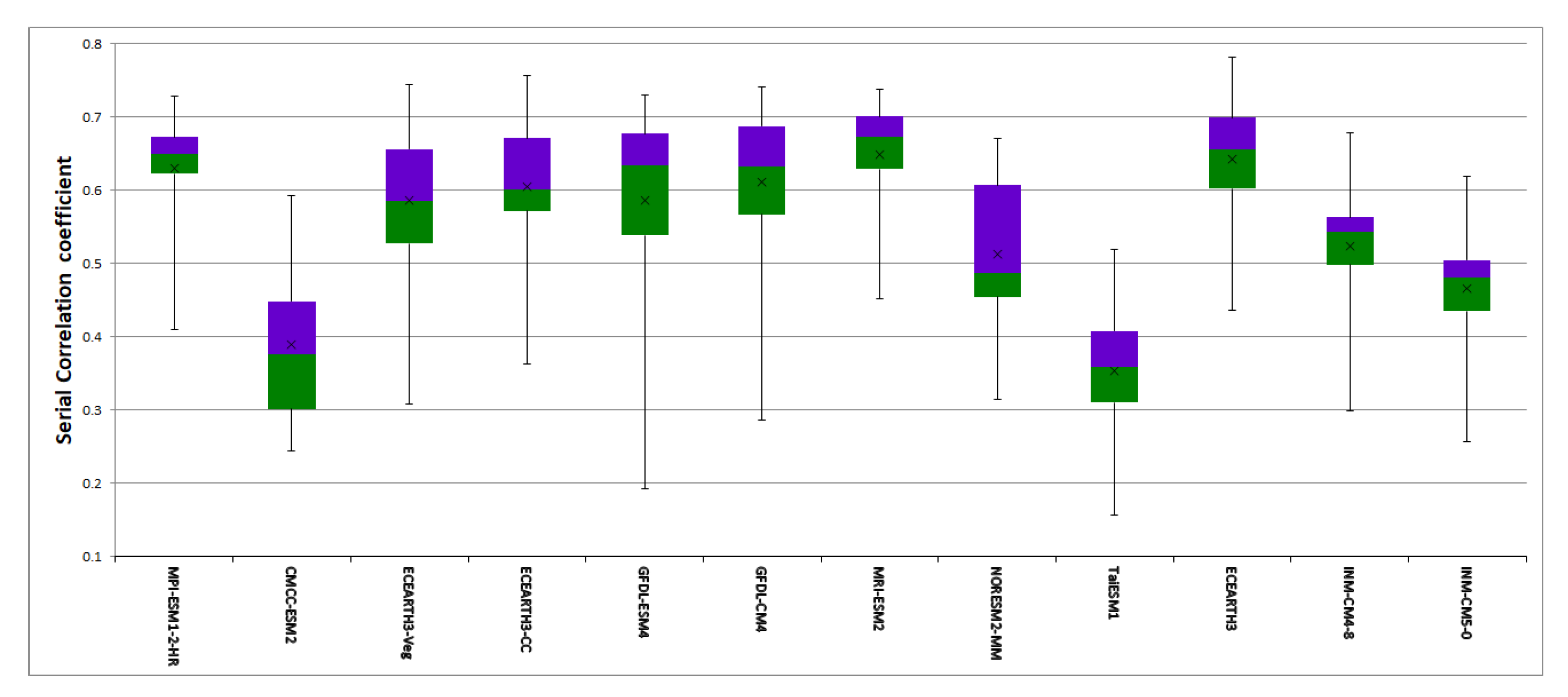
3.1.3. Performance Metrics

Four different performance indicators were implemented to identify models with good prediction capabilities across all time steps.

Table 5. Summary of model performances for all three climatic variables across four performance measures for the observed and climate model series.

			Ranks
Data Type	${\mathit{R}}^{\mathbf{2}}$	RMSE	MAE	BIAS	Sum of Rank
Precipitation
ECEARTH3	6	2	2	4	14
ECEARTH3-Veg	2	6	1	10	19
GFDL-ESM4	3	1	8	12	24
CMCC-ESM2	10	5	9	1	25
INM-CM4-8	1	10	7	8	26
NorESM2-MM	5	11	6	5	27
MPI-ESM1-2-HR	4	8	5	11	28
MRI-ESM2	9	9	3	7	28
TaiESM1	7	3	10	9	29
GFDL-CM4	8	4	12	6	30
INM-CM5.0	12	12	4	2	30
ECEARTH3-CC	11	7	11	3	32
Maximum Temperature
TaiESM1	6	1	1	3	11
INM-CM5-0	4	2	2	6	14
ECEARTH3	1	4	9	1	15
INM-CM4-8	7	3	3	4	17
ECEARTH3-CC	2	7	4	10	23
MPI-ESM1-2-HR	8	6	5	5	24
GFDL-ESM4	3	5	6	12	26
ECEARTH3-Veg	9	8	8	2	27
GFDL-CM4	10	9	7	7	33
MRI-ESM2	5	12	11	11	39
CMCC-ESM2	12	10	10	8	40
NorESM2-MM	11	11	12	9	43
Minimum Temperature
GFDL-CM4	4	1	1	1	7
MPI-ESM1-2-HR	1	2	3	11	17
TaiESM1	3	4	4	6	17
INM-CM4-8	5	3	2	12	22
ECEARTH3-Veg	2	8	8	7	25
INM-CM5-0	10	6	7	4	27
MRI-ESM2	12	7	5	3	27
GFDL-ESM4	9	5	6	10	30
CMCC-ESM2	6	9	9	8	32
NorESM2-MM	8	12	12	2	34
ECEARTH3	7	11	10	9	37
ECEARTH3-CC	11	10	11	5	37

shows the summarized results of each model across those four time steps against four performance measures. The ranking shown in the summary table for each performance measure was obtained by ranking the sum of ranks across each time step.

In the precipitation series, ECEARTH3-CC is the model that had a relatively poor overall performance in predicting the observed series. Moreover, the two other ECEARTH3 families were the top performers. For the maximum temperature series, the NorESM2-MM model performed poorly and TaiESM1 was the top-ranked model in terms of simulating the observed series, as shown in the summary of Table 5. From Table 5, it can also be observed that GFDL-CM4 and ECEARTH3-CC are models that performed well and poorly when simulating the observed minimum temperature series, respectively.

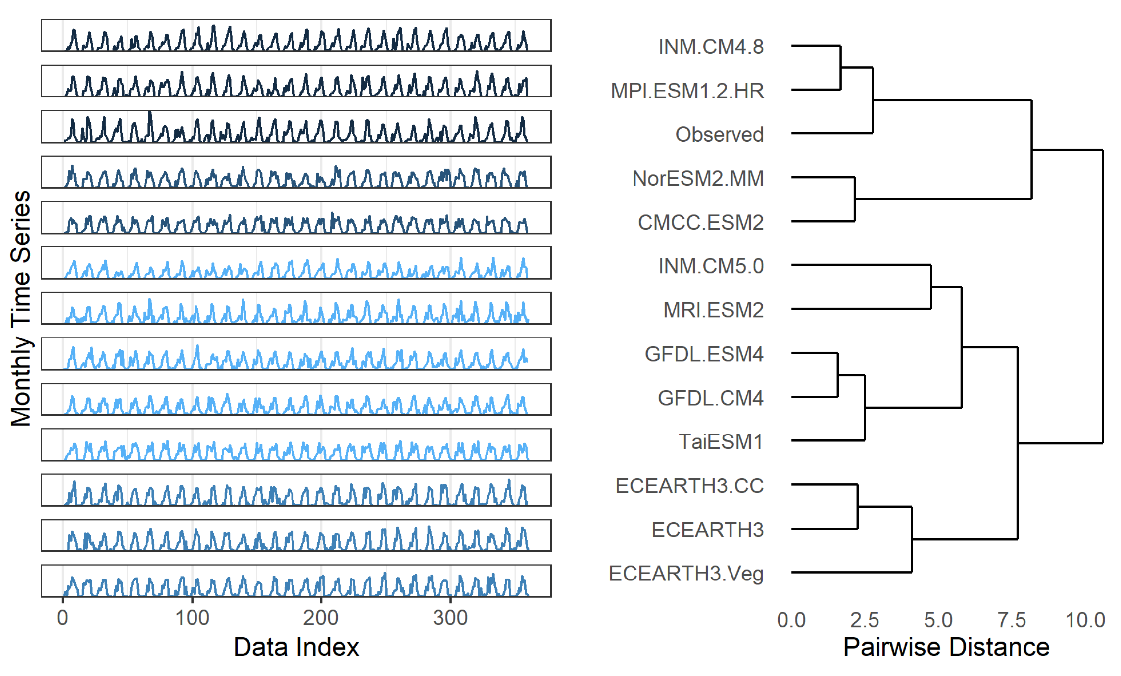
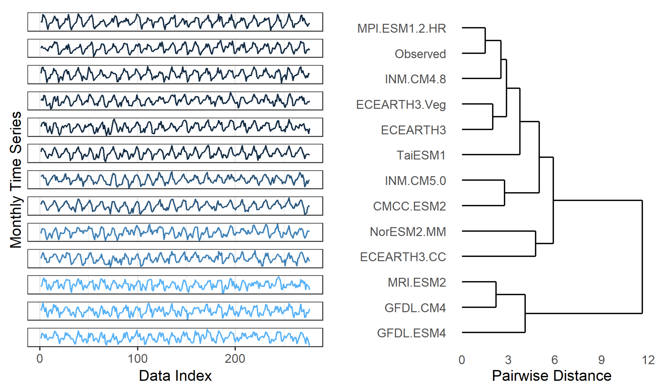
3.1.4. Time Series Clustering

A time-series clustering technique was used in order to identify which climate model was more capable of simulating the observed series in terms of capturing the seasonal variation. This technique uses a distance measure calculated from the cumulative periodograms of the observed and climate models. Using the distance matrix calculated from the integrated periodograms, a complete link agglomerative hierarchical clustering was performed on the monthly precipitation and maximum and minimum temperature series.

From Figure 3, it can be observed that for the precipitation series, the twelve models were clustered into four groups. Moreover, as expected, models that came from the same modeling institution, such as ECEARTH3 and GFDL families, were clustered together. It can be seen that two models, INM-CM4-8 and MPI-ESM1-2-HR, were able to be in the same cluster as the observed series, which means the two are good at simulating seasonal characteristics. Next in line, in terms of having closer seasonal characteristics to the observed series, were INM-CM5-0 and CMCC-ESM2. There was a clear sub-grouping with the rest of the models, which indicated less potential in simulating the seasonal behaviors of the observed series.

Similarly, for the monthly maximum temperature series, a clear clustering between models can be observed. Here, the same models, which are seen in the precipitation series, are the ones that have similar seasonal characteristics as shown in Figure 4.

The clustering of the monthly minimum temperature series is different from the two previous cases, as shown in Figure 5. Here, MRI-ESM2-0 and MPI-ESM1-2-HR performed well in capturing the seasonal variation. Additionally, the dissimilarities between the observed series, the ECEARTH3 family, and NorESM2-MM are relatively higher as compared to the rest of the climate models.

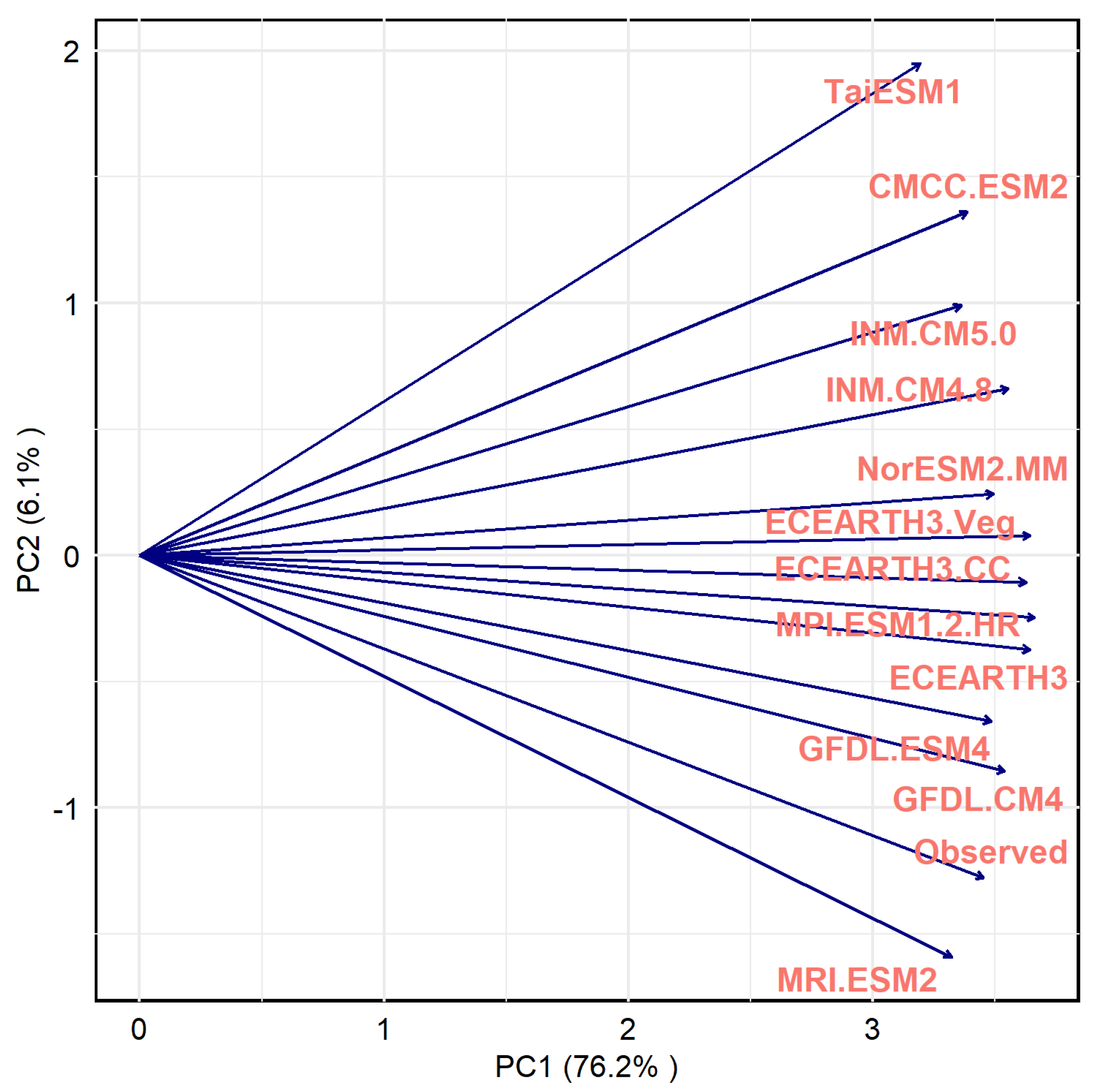
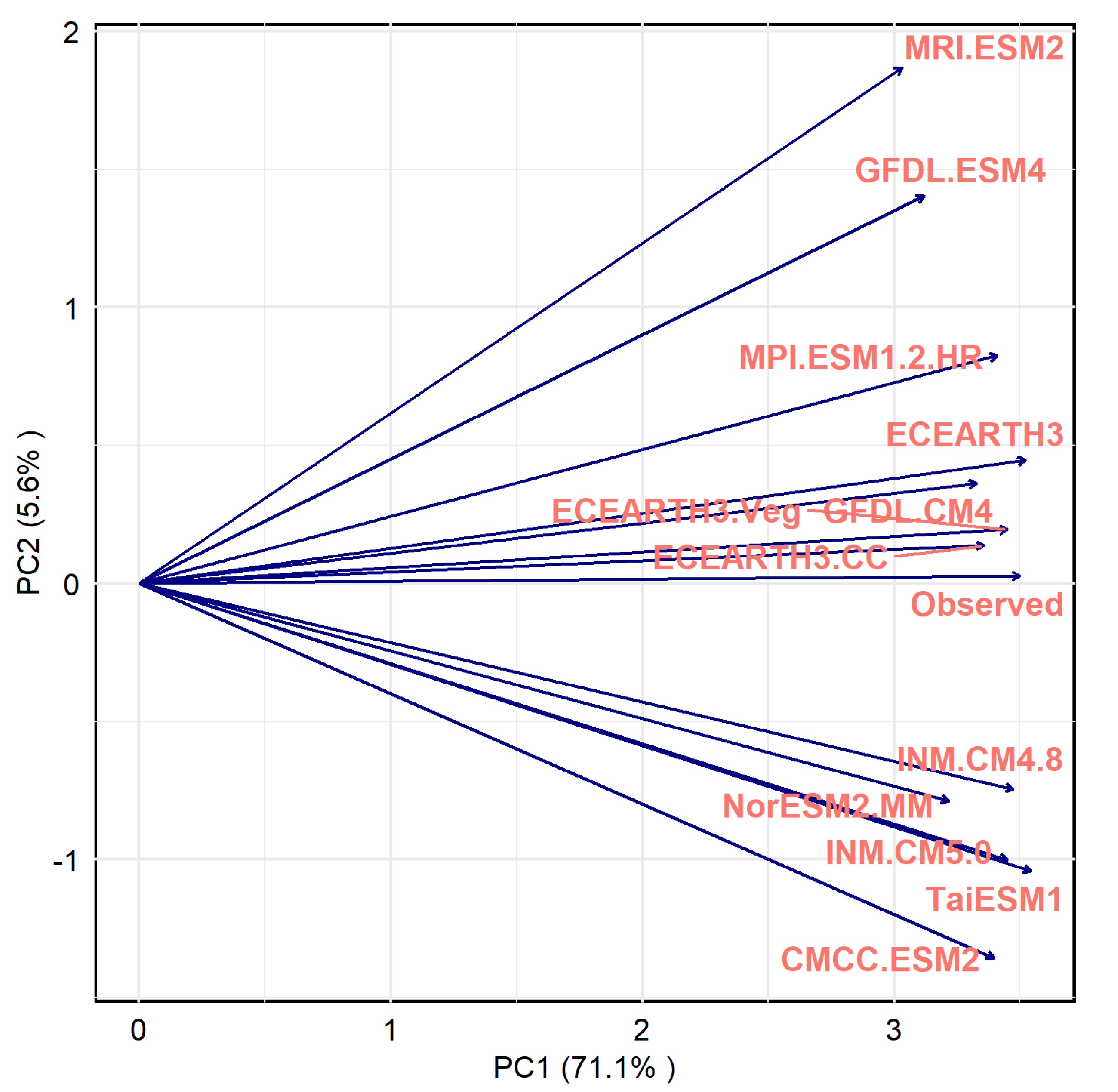
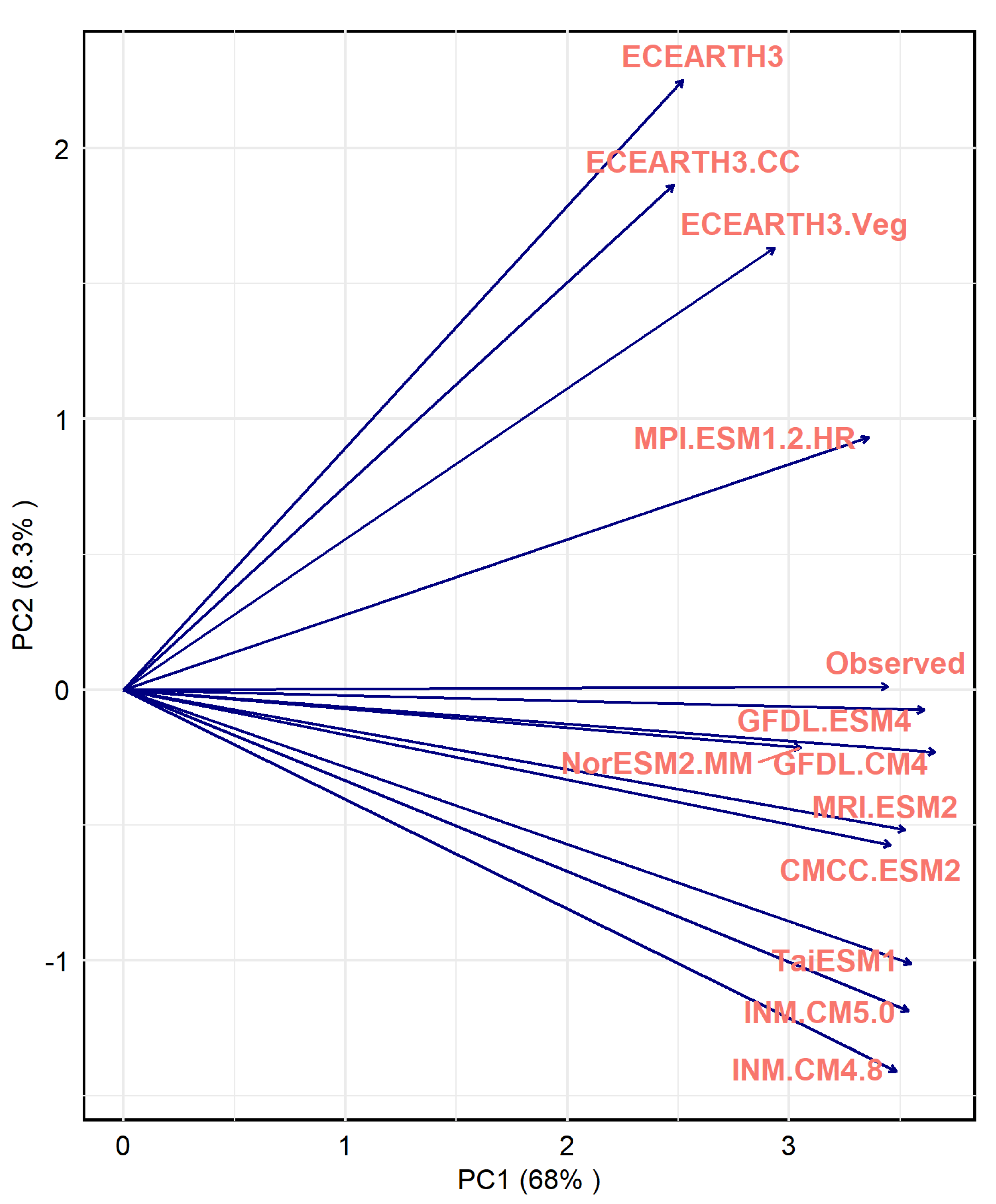
3.1.5. Principal Component Analysis (PCA)

From the PCA analysis of monthly precipitation data, most of the climate models were aligned along the PC1 with the exceptions of TaiESM1, CMCC-ESM2, and MRI-ESM2. Nearly all of the variances of models ECEARTH3-Veg and ECAERTH3-CC are explained by PC1. The models MPI-ESM1-2-HR and ECEARTH3 consist of one group that is closely correlated. As shown in Figure 6, the observed series is strongly correlated to MRI-ESM2.

The ECEARTH3 families and GFDL-CM4 showed good correlations with the observed maximum temperature series, as shown in Figure 7. The MRI-ESM2-0 and CMCC-ESM2 showed the least correlation.

Contrarily to the monthly maximum series, in the monthly minimum series, the ECEARTH3 families showed poor correlation. The most highly correlated model was GFDL-ESM4 followed by the groups of models that included GFDL-CM4, NorESM2-MM, and MRI-ESM2-0, as shown in Figure 8.

3.1.6. Spatial Performances of the Models

The spatial performances of the models were evaluated first by correlating the observed values and climate model outputs at each station for all three climatic variables. For example, Figure 9 shows the box plot of the monthly precipitation correlation coefficient values for each climate model at all stations. From this figure, we can infer that models MPI-ESM1-2-HR, ECEARTH3, and MRI-ESM2 had relatively better correlation to the observed monthly precipitations across the basin. Models CMCC-ESM2 and TaiESM1 were the poorly performing ones.

Similarly, the correlation box plots for the maximum temperature series (Figure 10) show that two models, MPI-ESM1-2-HR and ECEARTH3, were better correlated; MRI-ESM2 performed the poorest.

The correlation coefficient values for the minimum temperature (Figure 11) are not consistent with the precipitation and maximum temperature series. Here, models belonging to the GFDL family showed relatively good performances against the others, while the ECEARTH families had the lowest correlations.

In addition to the analysis of the spatial distribution of the correlation coefficients, RMSE was used to observe which climate model had the better model fit to the observed series. As can be observed from Figure 12, models GFDL-CM4, MRI-ESM2, and GFDL-ESM4 had less spatial RMSE values for the monthly precipitation when compared to the rest. INM-CM4-8 and TaiESM1 had the least spatial performances. In all models, there were fewer errors in simulating the rainfall of stations located at higher elevations.

3.2. Model Ranking and Interpretation

In the interpretation and summary of the results, a simple rank-based system was used. A higher rank (lowest in terms of magnitude) was given to a specific climate model for the desired effect. For example, in the interpretation of the results of the distribution fitting—if a specific model was fit with the same model as the observed series, then a value of one (unit) was assigned, and if otherwise, then zero. These values would be summed across the four analysis periods for each model and given a rank. The ranking was from one to twelve similar to the total number of climate models used in the study. A model had a higher rank in this case if the sum of ranks was higher.

A similar approach is also used in the interpretation of the trend analysis. That means, if a similar trend is obtained for a specific model, then a value of one is assigned, and zero if the contrary. The rest of the ranking procedure is the same as the one used in the interpretation of the distribution analysis. For the case of the performance measure, a higher rank was given to a specific model that scored well according to the criteria of each measure. Since four performance measures were used for each model, the final was based on ranking the sum of ranks.

To interpret the cluster analysis, the result of the distance (dissimilarity) matrix was used. A model with a minimum distance from the observed series was ranked higher than the one with a large distance. To summarize the PCA analysis, the angle between the loading vectors of the observed and climate models was used in the ranking criteria. Here, similarly among the ten models, a model with fewer angles was much closer to the observed series, so a higher-ranked was assigned to it. Finally, the areal-averaged values of two spatial measures (correlation and RMSE) were given a rank.

From the result of the precipitation time-series analysis across each method, the TaiESM1 model performed poorly, as shown in

Table 6. Summary rank based on seven criteria used for evaluating the three climate model time series.

Model	PDF Rank	Trend Rank	PM Rank	Cluster Rank	PCA Rank	SpatCorr	SpaRMSE	Sum of Rank	Final Rank
Precipitation
MRI-ESM2	1	1	8	6	1	1	3	21	1
GFDL-ESM4	5	1	3	4	3	5	2	23	2
MPI-ESM1-2-HR	5	1	7	1	5	4	4	27	3
GFDL-CM4	5	1	10	8	2	3	1	30	4
ECEARTH3	5	10	1	9	4	2	5	36	5
NorESM2-MM	2	1	6	5	8	8	8	38	6
ECEARTH3-Veg	5	1	2	12	7	7	7	41	7
INM-CM5-0	5	1	11	3	10	10	10	50	8
CMCC-ESM2	5	1	4	10	11	11	9	51	9
ECEARTH3-CC	4	10	12	7	6	6	6	51	9
INM-CM4-8	5	12	5	2	9	9	12	54	11
TaiESM1	2	1	9	11	12	12	11	58	12
Maximum Temperature
ECEARTH3	4	6	3	3	4	3	1	24	1
INM-CM5-0	4	2	2	5	8	4	3	28	2
INM-CM4-8	4	6	4	4	5	2	4	29	3
MPI-ESM1-2-HR	4	9	6	1	6	1	2	29	3
TaiESM1	4	2	1	2	9	7	8	33	5
ECEARTH3-CC	2	12	5	8	1	5	5	38	6
ECEARTH3-Veg	4	6	8	6	2	6	6	38	6
CMCC-ESM2	4	2	11	7	10	8	7	49	8
GFDL-CM4	1	9	9	11	3	9	9	51	9
GFDL-ESM4	2	1	7	10	11	10	10	51	9
NorESM2-MM	4	2	12	9	7	11	12	57	11
MRI-ESM2	4	9	10	12	12	12	11	70	12
Minimum Temperature
GFDL-CM4	2	1	1	4	2	1	1	12	1
MPI-ESM1-2-HR	1	5	2	1	6	6	7	28	2
TaiESM1	5	1	3	7	7	4	3	30	3
GFDL-ESM4	2	9	8	3	1	3	5	31	4
MRI-ESM2	5	9	7	2	4	2	2	31	4
CMCC-ESM2	2	1	9	5	5	8	8	38	6
INM-CM5-0	5	9	6	6	8	5	4	43	7
INM-CM4-8	5	7	4	8	9	7	9	49	8
NorESM2-MM	5	5	10	11	3	9	6	49	8
ECEARTH3-Veg	5	7	5	9	10	10	10	56	10
ECEARTH3-CC	5	1	12	10	11	11	11	61	11
ECEARTH3	5	9	11	12	12	12	12	73	12

NB: PDFR (PDF Rank), TrendR (Trend Rank), PMR (performance measure rank), ClusterR (cluster rank), PCAR (PCA rank), SpatCorr (spatial Correlation), SpaRMSE (spatial RMSE), SRank (sum of rank), FRank (final rank).

. The top three models that showed overall good performances were MRI-ESM2, GFDL-ESM4, and MPI-ESM1-2-HR.

There is no common model that has a good performance across the three climate variables as seen in Table 6. The poorest performance for the maximum temperature series was observed in MRI-ESM2. In the case of the minimum temperature series, the ECEARTH3 family performed poorly; contrarily, the GFDL family was one of the top performers, as shown in Table 6.

Finally, the ranking methodology was applied for the identification of possible models with overall good performances for all three climatic variables of concern, as shown in

Table 7. Summary results for all three climatic variables.

Data Type	Precip Rank	Tmax Rank	Tmin Rank	Sum of Rank	Final Rank
MPI-ESM1-2-HR	3	3	2	8	1
GFDL-CM4	4	9	1	14	2
GFDL-ESM4	2	9	4	15	3
INM-CM5-0	8	2	7	17	4
MRI-ESM2	1	12	4	17	4
ECEARTH3	5	1	12	18	6
TaiESM1	12	5	3	20	7
INM-CN4-8	11	3	8	22	8
CMCC-ESM2	9	8	6	23	9
ECEARTH3-Veg	7	6	10	23	9
NorESM2-MM	6	11	8	25	11
ECEARTH3-CC	9	6	11	26	12

. It can be observed that the MPI-ESM1-2-HR model is one of the models with the highest overall ranking when compared across the three climatic variables.

3.3. Future Climate Projections

In order to comment on the future climate conditions in the study area, the QM technique was applied as a tool to bias-adjust the top five climate models (MPI-ESM1-2-HR, GFDL-ESM4, INM-CM5-0, MRI-ESM2, and ECEARTH3). Future climate projections were done using an ensemble average of those five models. Because of the absence of the required scenarios, the GFDL-CM4 model was not used in future climate projection. In terms of the precipitation variables, for three time periods of analysis (near, middle, and end of the century), a general increase in the precipitation amount was observed (

Table 8. Mean annual areal-averaged future climate change over UASB for three time periods and two scenarios.

	Scenarios	Near	Mid	End
Precipitation (%$\Delta$)	SSP5-8.5	(−2.1–5.3) 1.3	(6.1–16.1) 10.6	(11.8–29.4) 19.7
	SSP2-4.5	(−0.7–6.8) 2.7	(2.0–11.9) 6.4	(2.2–15.0) 7.9
	SSP1-2.6	(−1.2–9.0) 3.4	(1.4–16.6) 8.2	(−0.3–14.2) 6.2
Tmax (°C)	SSP5-8.5	(0.8–1.5) 1.2	(1.7–2.3) 2.0	(2.8–3.2) 3.0
	SSP2-4.5	(0.7–1.5) 1.1	(1.3–2.0) 1.6	(1.7–2.3) 2.0
	SSP1-2.6	(0.7–1.4) 1.1	(0.9–1.7) 1.3	(0.9–1.8) 1.3
Tmin (°C)	SSP5-8.5	(1.0–1.9) 1.4	(2.2–2.9) 2.5	(3.7–4.2) 4.0
	SSP2-4.5	(1.0–1.7) 1.3	(1.6–2.3) 2.0	(2.1–2.7) 2.4
	SSP1-2.6	(0.9–1.7) 1.3	(1.2–2.0) 1.6	(1.1–2.0) 1.6

NB: numbers in the brackets indicate uncertainty limits of mean changes of the mean annuals calculated by using the standard deviation across the years of each series (predicted and observed).

) as compared to the base period (1980–2009). The magnitude of increment in the mean annual areal precipitation for the near, middle, and end of the century were 1.3%, 10.6%, and 19.7%, respectively, for the worst-case socioeconomic scenario. Moreover, for the middle socioeconomic scenario, increments of 2.7%, 6.4%, and 7.9% were seen for the near, middle, and end of the century, respectively. Here, except for the sustainable scenario, a higher magnitude of increments was expected by the end of this century. When the seasonal patterns of change were investigated, the magnitude of the increment for the spring rainfall was slightly higher than the summer, as shown in

Table 9. Seasonal areal-averaged precipitation future climate change (%$\Delta$) over UASB for three time periods and two scenarios.

		MAM			JJAS
	Near	Mid	End	Near	Mid	End
SSP5-8.5	(−0.15–0.46) 0.03	(−0.10–0.47) 0.08	(−0.04–0.58) 0.15	(−0.12–0.02) −0.06	(−0.06–0.11) 0.01	(0.02–0.16) 0.08
SSP2-4.5	(−0.13 −0.6) 0.08	(−0.08–0.45) 0.09	(−0.11–0.48) 0.08	(−0.11–0.04) −0.04	(−0.10–0.07) −0.02	(−0.06–0.08) 0.00
SSP1-2.6	(−0.14–0.6) 0.07	(−0.06–0.56) 0.14	(−0.07–0.43) 0.09	(−0.11–0.06) −0.04	(−0.09–0.09) −0.01	(−0.08–0.07) −0.02

. Here, we can see a predicted decrement in the summer rainfall, especially for the near-time period.

The mean annual areal maximum temperature in the middle scenario showed increments of 1.1 °C, 1.6 °C, and 2.0 °C for the near, middle, and end of the century, respectively. With the same pattern, increases of 1.2 °C, 2.0 °C, and 3.0 °C were seen for the worst case, respectively. Similarly, for the minimum temperature series in the middle scenario, increases of 1.3 °C, 2.0 °C, and 2.4 °C were observed for near, middle, and end of the century, respectively. The worst-case scenario showed increments of 1.4 °C, 2.5 °C, and 4.0 °C for the near, middle, and end of the century, respectively. It can be concluded that—similar to the precipitation variable—higher magnitudes of temperature increments are observed at the end of the century. Moreover, the increment amounts are relatively higher for minimum temperature than the maximum temperature.

The results of the future climate analysis discussed in the previous two paragraphs indicate the areal-averaged outputs only. In order to understand how the changing pattern may look spatially, four representative stations were selected across the basin. The relative geographic locations (north, east, south, west) in the sub-basin were the main criteria for selections; the intention was to observe if there was any spatial pattern in future climate across the sub-basin.

Analysis of future precipitation (

Table 10. Mean annual future climate change at the selected four meteorological stations in the UASB for the three time periods and two scenarios.

Stations	Scenarios	Near	Mid	End
		Precip (%$\Delta$)
AA	SSP5-8.5	(4.3–9.7) 7.4	(6.0–25.9) 17.5	(28.6–33.2) 31.3
	SSP2-4.5	(24.6–26.3) 25.3	(10.5–13.3) 11.7	(10.0–10.0) 10.0
Ejere	SSP5-8.5	(−1.6–13.2) 3.8	(21.1–23.9) 22.8	(29.7–46.9) 36.2
	SSP2-4.5	(11.1–37.9) 20.9	(5.2–28.7) 14.0	(6.9–24.1) 13.4
Hombole	SSP5-8.5	(−23.4–63.7) −2.6	(3.4–77.7) 22.0	(7.5–123.3) 36.6
	SSP2-4.5	(−14.5–93.9) 11.4	(−12.5–93.7) 14.1	(−12.0–86.1) 12.6
Ginchi	SSP5-8.5	(−3.3–5.1) −0.1	(14.2–15.1) 14.6	(18.0–34.6) 24.5
	SSP2-4.5	(6.3–26.5) 14.1	(2.3–17.8) 8.4	(0.2–21.3) 8.5
		Tmax (°C)
AA	SSP5-8.5	(1.0–1.3) 1.2	(2.4–2.4) 2.4	(3.3–3.6) 3.5
	SSP2-4.5	(0.8–0.9) 0.8	(2.1–2.3) 2.2	(2.6–2.8) 2.7
Bui	SSP5-8.5	(0.6–2.1) 1.3	(2.4–3.4) 2.9	(3.8–4.6) 4.2
	SSP2-4.5	(0.5–1.6) 1.1	(2.1–3.3) 2.7	(2.7–4.0) 3.3
Debrezeit	SSP5-8.5	(1.3–1.5) 1.4	(2.9–3.2) 3.0	(4.0–4.6) 4.3
	SSP2-4.5	(1.0 -1.1) 1.1	(2.7–2.8) 2.7	(3.5–3.5) 3.5
Tulubolo	SSP5-8.5	(−0.1–2.8) 1.4	(1.3–3.8) 2.6	(2.5–4.9) 3.7
	SSP2-4.5	(−0.3–2.5) 1.1	(1.0–3.8) 2.4	(1.5–4.4) 3.0
		Tmin (°C)
AA	SSP5-8.5	(1.5–1.7) 1.6	(2.6–2.7) 2.7	(3.8–4.4) 4.1
	SSP2-4.5	(1.1–1.2) 1.2	(2.2–2.3) 2.2	(2.6–3.0) 2.8
Bui	SSP5-8.5	(1.3–3.8) 2.5	(3.5–5.4) 4.5	(5.4–7.0) 6.2
	SSP2-4.5	(1.0–3.0) 2.0	(2.9–5.1) 4.0	(3.3–5.8) 4.6
Debrezeit	SSP5-8.5	(1.5–1.9) 1.7	(3.2–3.3) 3.2	(4.4–4.9) 4.7
	SSP2-4.5	(1.2–1.3) 1.2	(2.7–2.8) 2.8	(3.1–3.6) 3.3
Tulubolo	SSP5-8.5	(0.9–1.8) 1.4	(1.9–4.1) 3.0	(3.2–5.2) 4.2
	SSP2-4.5	(0.8–1.4) 1.1	(1.4–3.9) 2.7	(1.8–4.5) 3.1

) shows that there seems to be a relatively higher precipitation mean change and larger uncertainty in the mean change prediction for stations Ejere and Hombole. In the case of future temperature changes, stations Deberzeit and Bui had higher changes when compared to the other two stations. Moreover, stations Bui and Tulubolo had larger uncertainties in predicting the mean change for both maximum and minimum temperature series. There was no clear spatial pattern to observe in the change of future precipitation across the sub-basin. However, the future changes in temperature values show that stations located at lower elevations had higher relative changes.

4. Discussion

Models that are incorporated in the new CMIP6 archive showed comparable or improved capabilities in terms of simulating the climate of the globe as compared to CMIP5 [55]. This is because the models in the CMIP6 archive showed improved model resolution, setups, scenarios, and parametrization compared to all previous CMIP versions [18]. This study mainly focused on the application of statistical and data mining techniques to identify possible climate models from the new CMIP6 archive, which can simulate the climate system of UASB. This was made possible after evaluating all models against the observed historical climate series using the mentioned evaluation criteria. All comparisons were performed on spatially averaged data for the 1980–2009 period of analysis.

No specific model had a consistent performance across the evaluation criteria and climatic variables as shown in Table 6. Model MRI-ESM2-0 represented the distributional properties of the precipitation series. GFDL-CM4 and MPI-ESM1-2-HR performed well for the minimum and maximum temperature series, respectively. In terms of capturing the trend behavior the GFDL-ESM4 model performed equally well for the precipitation and maximum temperature series; models GFDL-CM4, TaiESM1, CMCC-ESM2, and ECEARTH3-CC had equal potential for the minimum temperature series. The outputs of the model fit performance measures indicated that no specific models had similar performances across the three climate variables. The seasonal patterns were better captured by MPI-ESM1-HR for all three climate variables. Not all three climate variables were correlated to the same climate models in the PCA analysis. MRI-ESM2, EC-EARTH3-CC, and GFDL-ESM4 had better correlations with the precipitation, maximum temperature, and minimum temperature series, respectively.

The results of the two spatial evaluation criteria indicate that MRI-ESM2 had better spatial correlation but GFDL-CM4 was a good model fit for the precipitation series. MPI-ESM1-2-HR and ECEARTH3 ranked the highest for the maximum temperature serious based on those criteria, respectively. In addition, the GFDL-CM4 model ranked number one in the minimum temperature series for both criteria.

According to a recent study by [56], the summer rainfall over Ethiopia is influenced by SST conditions over the Gulf of Guinea and the southern Pacific Ocean. The spring rainfall was influenced by SST over the North Atlantic Ocean. A study by [57] indicated that the summer rainfall season (JAS) climate system over the UASB is highly influenced by the equatorial pacific ocean temperature. ENSO and ITCZ that arise from the ocean temperature variations over the equatorial pacific and low-pressure zone near the equator are also two important climate conditions that shape the climate over UASB.

Most of the climate models evaluated in this study have different performances in terms of simulating the global climate process. A recent work presented by [55] showed that models EC-EARTH3, MPI-ESM1-2-HR, and TaiESM1 have good capabilities in terms of capturing ENSO teleconnections. The MPI-ESM1-2-HR model is also capable of producing teleconnections over the Indian and North Atlantic oceans reasonably well [58]. As shown in the results section, the models are among the top-ranked models in this study.

Another important reason why the top-ranked MPI-ESM1-2-HR model performed well may be due to the fact that it has higher atmospheric and ocean model resolutions relative to the ten models. This model has 0.94${}^{°}$atmospheric resolution with 95 verticals and the model top at 0.01 hPa. Moreover, the ocean model is having 0.4${}^{°}$ horizontal resolution with 40 levels [58,59]. The poorest performing model, which was CMCC-ESM2, has an atmospheric resolution of 0.9${}^{°}$× 1.25${}^{°}$ with 30 verticals and a model top at 2 hPa. Moreover, the ocean model has a resolution of 0.33${}^{°}$ [60]. Since the topography of the study area is complex, it is expected that the model resolution plays a vital role in capturing all important climate characteristics of the study area.

Past climate change studies on the basin that applied CMIP5 outputs have all predicted an increase in temperatures for all time periods and scenarios [33,34,35]. However, there is no clear agreement on future precipitation changes. The works by Taye et al. [33] and Tadese et al. [34] have indicated an increase in the summer (JJAS) and a decrease in the spring (MAM) rainfalls for both the 2050s and 2070s and two scenarios (RCP4.5 and RCP8.5). Daba and You [35] predicted an increase in summer rainfall for the 2020s and a decrease in both the summer and spring rainfalls for the 2050s and 2080s for those two same scenarios. However, the previous AR5 for CMIP5 and the new AR6 for the CMIP6 IPCC reports predict that there will be increases in the annual mean precipitation and maximum temperature values for both the mid and end of the century over East Africa [61,62]. So, it can be seen that the findings from these previous studies are in disagreement with the IPCC report. These fallacies may be due to the poor performances of these previous climate models in simulating the climate conditions over East Africa or improper model selections. In this study, it was predicted that there are increases in both precipitation and temperature Table 8 presents different magnitudes for three scenarios, especially for the mid- and far-time periods. Contrary to CMIP5 outputs, it was found that there is a slightly higher increment in the spring rainfall than in the summer. In addition, the uncertainty bands of future precipitation changes indicate a relatively larger uncertainty toward the end-of-century, while for the temperature series, the reverse is true. This might be due to the characteristics of precipitation prediction, which makes them more likely to be influenced by local factors than temperature. It can be observed that all of the findings of this study on future climate projections align with the new AR6 IPCC report on future climate conditions over Northeast Africa [62].

5. Conclusions

The outputs of the selection process have indicated that it is difficult to conclude the performance of a single model since the performance of each model is different for each evaluation criterion. However, the MPI-ESM1-2-HR model showed an overall good performance when evaluated for all time steps and evaluation criteria.

When observing the outputs of each evaluation criterion across the three climatic variables, the GFDL-CM4 model seems to be the best model across the three measures (PDF, PCA, and spatial). The second evaluation criteria for trend behavior shows that the CMCC-ESM2 model could capture the trend well. Outputs of model fit performance measures ($R^2$, RMSE, MAE, and BIAS) indicate that INM-CM4-8 outperformed the others. MPI-ESM1-2-HR is the best model in terms of capturing the stochastic behavior (underlying periodic patterns) of the observed series.

Downscaling and bias adjustment to the scenarios obtained from the top five high-ranking models (ECAERTH3, GFDL-ESM4, MPI-ESM1-2-HR, MRI-ESM2, and INM-CM5-0) were performed using the IDW and QM approaches for all three climate variables (precipitation, maximum temperature, and minimum temperature). Based on the results of downscaling and bias adjustment, predictions of future climate conditions for three socioeconomic scenarios (sustainable, middle, and worst) across three time periods (near, middle, and end of the century) were conducted. The results of future climate prediction showed relative increments compared to the base period (1980–2009) for all three climate variables. The magnitude of the increment was relatively higher for the end than near the middle of this century. In addition, the analysis of seasonal projection indicated that the magnitude of the increment for spring rainfall was higher than for the summer. It can be observed that outputs of this study are in agreement with the new AR6 IPCC report about expected future climate changes in Northeast Africa.

The intensifying agricultural activity and urbanization in the study area [7] with the projected increase in precipitation amount could lead to higher risks of flooding over UASB in the future.

The results of this study could be verified through the inclusion of other ensemble variants in addition to r1i1p1f1.

References

1. Water, C. Leaving No One Behind. In The United Nations World Water Development Report Paris; UNESCO: Paris, France, 2019. [Google Scholar]
2. Gleick, P.H. Water in Crisis; Oxford University Press: New York, NY, USA, 1993; Volume 100. [Google Scholar]
3. Thakural, L.; Kumar, S.; Jain, S.K.; Ahmad, T. The impact of climate change on rainfall variability: A study in central himalayas. In Climate Change Impacts; Springer: Singapore, 2018; pp. 181–192. [Google Scholar]
4. Shaaban, F.; Othman, A.; Habeebullah, T.M.; El-Saoud, W.A. An integrated GPR and geoinformatics approach for assessing potential risks of flash floods on high-voltage towers, Makkah, Saudi Arabia. Environ. Earth Sci. 2021, 80, 1–15. [Google Scholar] [CrossRef]
5. Claire, S.; Denise, G. DroughtScape. 2019, pp. 3–6. Available online: https://digitalcommons.unl.edu/cgi/viewcontent.cgi?article=1052&context=droughtscape (accessed on 14 November 2022).
6. NMA. Climate Change National Adaptation Programme of Action (NAPA) of Ethiopia; National Meteorological Services Agency (NMA), Ministry of Water Resources, Federal Democratic Republic of Ethiopia: Addis Ababa, Ethiopia, 2007. [Google Scholar]
7. Shawul, A.A.; Chakma, S. Spatiotemporal detection of land use/land cover change in the large basin using integrated approaches of remote sensing and GIS in the Upper Awash basin, Ethiopia. Environ. Earth Sci. 2019, 78, 1–13. [Google Scholar] [CrossRef]
8. Nanesa, K. Awash River’s the Ongoing Irrigation Practices, Future Projects and its Impacts on the Environment of Awash River Basin. Irrig. Drain. Syst. Eng. 2021, 10. [Google Scholar] [CrossRef]
9. Aregahegn, Z.; Zerihun, M. Study on Irrigation Water Quality in the Rift Valley Areas of Awash River Basin, Ethiopia. Appl. Environ. Soil Sci. 2021, 2021, 8844745. [Google Scholar] [CrossRef]
10. Mersha, A.N.; de Fraiture, C.; Masih, I.; Alamirew, T. Dilemmas of integrated water resources management implementation in the Awash River Basin, Ethiopia: Irrigation development versus environmental flows. Water Environ. J. 2021, 35, 402–416. [Google Scholar] [CrossRef]
11. Edossa, D.C.; Babel, M.S.; Gupta, A.D. Drought analysis in the Awash river basin, Ethiopia. Water Resour. Manag. 2010, 24, 1441–1460. [Google Scholar] [CrossRef]
12. Shenduli, P.R.; Van Andel, S.J.; Mamo, S.; Masih, I. Improving hydrological prediction with global datasets: Experiences with Brahmaputra, Upper Awash and Kaap catchments. In Proceedings of the E-Proceedings of the 37th IAHR World Congress, Kuala Lumpur, Malaysia, 13–18 August 2017. [Google Scholar]
13. Edwards, P.N. History of climate modeling. Wiley Interdiscip. Rev. Clim. Chang. 2011, 2, 128–139. [Google Scholar] [CrossRef] [Green Version]
14. Bhuvandas, N.; Timbadiya, P.V.; Patel, P.L.; Porey, P.D. Review of downscaling methods in climate change and their role in hydrological studies. Int. J. Environ. Ecol. Geol. Mar. Eng. 2014, 8, 713–718. [Google Scholar]
15. Soriano, E.; Mediero, L.; Garijo, C. Selection of bias correction methods to assess the impact of climate change on flood frequency curves. Water 2019, 11, 2266. [Google Scholar] [CrossRef] [Green Version]
16. Lutz, A.F.; ter Maat, H.W.; Biemans, H.; Shrestha, A.B.; Wester, P.; Immerzeel, W.W. Selecting representative climate models for climate change impact studies: An advanced envelope-based selection approach. Int. J. Climatol. 2016, 36, 3988–4005. [Google Scholar] [CrossRef] [Green Version]
17. Brief, C. How Do Climate Models Work? 2018. Available online: https://www.carbonbrief.org/qa-how-do-climate-models-work/ (accessed on 17 August 2021).
18. Ayugi, B.; Zhihong, J.; Zhu, H.; Ngoma, H.; Babaousmail, H.; Rizwan, K.; Dike, V. Comparison of CMIP6 and CMIP5 models in simulating mean and extreme precipitation over East Africa. Int. J. Climatol. 2021, 41, 6474–6496. [Google Scholar] [CrossRef]
19. Wilby, R. Evaluating climate model outputs for hydrological applications. Hydrol. Sci. J. J. Des. Sci. Hydrol. 2010, 55, 1090–1093. [Google Scholar] [CrossRef]
20. Khayyun, T.S.; Alwan, I.A.; Hayder, A.M. Selection of suitable precipitation CMIP-5 sets of GCMs for Iraq using a symmetrical uncertainty filter. In Proceedings of the IOP Conference Series: Materials Science and Engineering; IOP Publishing: Bristol, UK, 2020; Volume 671, p. 012013. [Google Scholar]
21. Homsi, R.; Shiru, M.S.; Shahid, S.; Ismail, T.; Harun, S.B.; Al-Ansari, N.; Chau, K.W.; Yaseen, Z.M. Precipitation projection using a CMIP5 GCM ensemble model: A regional investigation of Syria. Eng. Appl. Comput. Fluid Mech. 2020, 14, 90–106. [Google Scholar] [CrossRef]
22. Samadi, S.Z.; Sagareswar, G.; Tajiki, M. Comparison of general circulation models: Methodology for selecting the best GCM in Kermanshah Synoptic Station, Iran. Int. J. Glob. Warm. 2010, 2, 347–365. [Google Scholar] [CrossRef]
23. Pitman, A.; Perkins, S. Reducing uncertainty in selecting climate models for hydrological impact assessments. IAHS Publ. 2007, 313, 3. [Google Scholar]
24. Alemseged, T.H.; Tom, R. Evaluation of regional climate model simulations of rainfall over the Upper Blue Nile basin. Atmos. Res. 2015, 161, 57–64. [Google Scholar] [CrossRef]
25. Ongoma, V.; Chen, H.; Gao, C. Evaluation of CMIP5 twentieth century rainfall simulation over the equatorial East Africa. Theor. Appl. Climatol. 2019, 135, 893–910. [Google Scholar] [CrossRef]
26. Nashwan, M.S.; Shahid, S. Symmetrical uncertainty and random forest for the evaluation of gridded precipitation and temperature data. Atmos. Res. 2019, 230, 104632. [Google Scholar] [CrossRef]
27. Ahmadalipour, A.; Rana, A.; Moradkhani, H.; Sharma, A. Multi-criteria evaluation of CMIP5 GCMs for climate change impact analysis. Theor. Appl. Climatol. 2017, 128, 71–87. [Google Scholar] [CrossRef] [Green Version]
28. Rana, A.; Madan, S.; Bengtsson, L. Performance evaluation of regional climate models (RCMs) in determining precipitation characteristics for Gothenburg, Sweden. Hydrol. Res. 2014, 45, 703–714. [Google Scholar] [CrossRef]
29. Wilcke, R.A.; Bärring, L. Selecting regional climate scenarios for impact modelling studies. Environ. Model. Softw. 2016, 78, 191–201. [Google Scholar] [CrossRef] [Green Version]
30. Friedman, J.H. Data Mining and Statistics: What’s the connection? Comput. Sci. Stat. 1998, 29, 3–9. [Google Scholar]
31. Srinivasa Raju, K.; Nagesh Kumar, D. Ranking general circulation models for India using TOPSIS. J. Water Clim. Chang. 2015, 6, 288–299. [Google Scholar] [CrossRef]
32. Hailemariam, K. Impact of climate change on the water resources of Awash River Basin, Ethiopia. Clim. Res. 1999, 12, 91–96. [Google Scholar] [CrossRef] [Green Version]
33. Taye, M.T.; Dyer, E.; Hirpa, F.A.; Charles, K. Climate change impact on water resources in the Awash basin, Ethiopia. Water 2018, 10, 1560. [Google Scholar] [CrossRef] [Green Version]
34. Tadese, M.T.; Kumar, L.; Koech, R. Climate change projections in the Awash River Basin of Ethiopia using Global and Regional climate models. Int. J. Climatol. 2020, 40, 3649–3666. [Google Scholar] [CrossRef]
35. Daba, M.H.; You, S. Assessment of climate change impacts on river flow regimes in the upstream of Awash Basin, Ethiopia: Based on IPCC fifth assessment report (AR5) climate change scenarios. Hydrology 2020, 7, 98. [Google Scholar] [CrossRef]
36. Bussi, G.; Whitehead, P.G.; Jin, L.; Taye, M.T.; Dyer, E.; Hirpa, F.A.; Yimer, Y.A.; Charles, K.J. Impacts of Climate Change and Population Growth on River Nutrient Loads in a Data Scarce Region: The Upper Awash River (Ethiopia). Sustainability 2021, 13, 1254. [Google Scholar] [CrossRef]
37. Emiru, N.C.; Recha, J.W.; Thompson, J.R.; Belay, A.; Aynekulu, E.; Manyevere, A.; Demissie, T.D.; Osano, P.M.; Hussein, J.; Molla, M.B.; et al. Impact of Climate Change on the Hydrology of the Upper Awash River Basin, Ethiopia. Hydrology 2022, 9, 3. [Google Scholar] [CrossRef]
38. Gebresellase, S.H.; Wu, Z.; Xu, H.; Muhammad, W.I. Evaluation and selection of CMIP6 climate models in Upper Awash Basin (UBA), Ethiopia. Theor. Appl. Climatol. 2022, 149, 1521–1547. [Google Scholar] [CrossRef]
39. Schulzweida, U. CDO User Guide. 2021. Available online: https://zenodo.org/record/5614769#.Y3wxceRBxPY (accessed on 14 November 2022). [CrossRef]
40. Rigby, R.A.; Stasinopoulos, D.M. Generalized additive models for location, scale and shape,(with discussion). Appl. Stat. 2005, 54, 507–554. [Google Scholar] [CrossRef] [Green Version]
41. R Core Team. R: A Language and Environment for Statistical Computing; R Foundation for Statistical Computing: Vienna, Austria, 2021. [Google Scholar]
42. Mann, H.B. Nonparametric Tests against Trend. Econometrica 1945, 13, 245–259. [Google Scholar] [CrossRef]
43. Yue, S.; Wang, C. The Mann-Kendall test modified by effective sample size to detect trend in serially correlated hydrological series. Water Resour. Manag. 2004, 18, 201–218. [Google Scholar] [CrossRef]
44. Sen, P.K. Estimates of the regression coefficient based on Kendall’s tau. J. Am. Stat. Assoc. 1968, 63, 1379–1389. [Google Scholar] [CrossRef]
45. De Lucas, D.C. Classification Techniques for Time Series and Functional Data. Ph.D. Thesis, Universidad Carlos III de Madrid, Madrid, Spain, 2010. [Google Scholar]
46. Montero, P.; Vilar, J.A. TSclust: An R Package for Time Series Clustering. J. Stat. Softw. 2014, 62, 1–43. [Google Scholar] [CrossRef] [Green Version]
47. Kabacoff, R.I. R in Action: Data Analysis and Graphics with R; Manning Publishings Co.: New York, NY, USA, 2015. [Google Scholar]
48. Hartmann, K.; Krois, J.; Waske, B. E-Learning Project SOGA: Statistics and Geospatial Data Analysis; Department of Earth Sciences, Freie Universitaet Berlin: Berlin, Germany, 2018; Volume 33. [Google Scholar]
49. Sarvina, Y.; Pluntke, T.; Bernhofer, C. Comparing bias correction methods to improve modelled precipitation extremes. J. Meteorol. Dan Geofis. 2019, 19, 103–110. [Google Scholar] [CrossRef]
50. Gudmundsson, L.; Bremnes, J.B.; Haugen, J.E.; Engen-Skaugen, T. Downscaling RCM precipitation to the station scale using statistical transformations—A comparison of methods. Hydrol. Earth Syst. Sci. 2012, 16, 3383–3390. [Google Scholar] [CrossRef] [Green Version]
51. Tabari, H.; Paz, S.M.; Buekenhout, D.; Willems, P. Comparison of statistical downscaling methods for climate change impact analysis on precipitation-driven drought. Hydrol. Earth Syst. Sci. 2021, 25, 3493–3517. [Google Scholar] [CrossRef]
52. Maraun, D. Bias correcting climate change simulations-a critical review. Curr. Clim. Chang. Rep. 2016, 2, 211–220. [Google Scholar] [CrossRef] [Green Version]
53. Iturbide, M.; Bedia, J.; Herrera, S.; Baño-Medina, J.; Fernández, J.; Frías, M.; Manzanas, R.; San-Martín, D.; Cimadevilla, E.; Cofiño, A.; et al. climate4r: An r-based open framework for reproducible climate data access and post-processing. Environ. Modell. Softw. 2018. [Google Scholar] [CrossRef]
54. Boé, J.; Terray, L.; Habets, F.; Martin, E. Statistical and dynamical downscaling of the Seine basin climate for hydro-meteorological studies. Int. J. Climatol. J. R. Meteorol. Soc. 2007, 27, 1643–1655. [Google Scholar] [CrossRef]
55. Planton, Y.Y.; Guilyardi, E.; Wittenberg, A.T.; Lee, J.; Gleckler, P.J.; Bayr, T.; McGregor, S.; McPhaden, M.J.; Power, S.; Roehrig, R.; et al. Evaluating climate models with the CLIVAR 2020 ENSO metrics package. Bull. Am. Meteorol. Soc. 2021, 102, E193–E217. [Google Scholar] [CrossRef]
56. Alhamshry, A.; Fenta, A.A.; Yasuda, H.; Kimura, R.; Shimizu, K. Seasonal rainfall variability in Ethiopia and its long-term link to global sea surface temperatures. Water 2020, 12, 55. [Google Scholar] [CrossRef] [Green Version]
57. Taye, M.T.; Dyer, E.; Charles, K.J.; Hirons, L.C. Potential predictability of the Ethiopian summer rains: Understanding local variations and their implications for water management decisions. Sci. Total Environ. 2021, 755, 142604. [Google Scholar] [CrossRef]
58. Jungclaus, J.; Fischer, N.; Haak, H.; Lohmann, K.; Marotzke, J.; Matei, D.; Mikolajewicz, U.; Notz, D.; Von Storch, J. Characteristics of the ocean simulations in the Max Planck Institute Ocean Model (MPIOM) the ocean component of the MPI-Earth system model. J. Adv. Model. Earth Syst. 2013, 5, 422–446. [Google Scholar] [CrossRef]
59. Gutjahr, O.; Putrasahan, D.; Lohmann, K.; Jungclaus, J.H.; von Storch, J.S.; Brüggemann, N.; Haak, H.; Stössel, A. Max planck institute earth system model (MPI-ESM1. 2) for the high-resolution model intercomparison project (HighResMIP). Geosci. Model Dev. 2019, 12, 3241–3281. [Google Scholar] [CrossRef] [Green Version]
60. Cherchi, A.; Fogli, P.G.; Lovato, T.; Peano, D.; Iovino, D.; Gualdi, S.; Masina, S.; Scoccimarro, E.; Materia, S.; Bellucci, A.; et al. Global mean climate and main patterns of variability in the CMCC-CM2 coupled model. J. Adv. Model. Earth Syst. 2019, 11, 185–209. [Google Scholar] [CrossRef] [Green Version]
61. Stocker, T.F.; Qin, D.; Plattner, G.K.; Tignor, M.; Allen, S.K.; Boschung, J.; Nauels, A.; Xia, Y.; Bex, B.; Midgley, B. IPCC 2013: Climate Change 2013: The Physical Science Basis, Contribution of Working Group I to the Fifth Assessment Report of the Intergovernmental Panel on Climate Change; Cambridge University Press: Cambridge, UK; New York, NY, USA, 2013; p. 1535. [Google Scholar]
62. Masson-Delmotte, V.; Zhai, P.; Pirani, A.; Connors, S.; Péan, C.; Berger, S.; Caud, N.; Chen, Y.; Goldfarb, L.; Gomis, M.; et al. IPCC 2021: The Physical Science Basis, Contribution of Working Group I to the Sixth Assessment Report of the Intergovernmental Panel on Climate Change; Cambridge University Press: Cambridge, UK; New York, NY, USA, 2021; p. 2391. [Google Scholar] [CrossRef]
63. Stasinopoulos, M.; Rigby, B.; Akantziliotou, C. Instructions on How to Use the Gamlss Package in R, 2nd ed.; Gamlss: London, UK, 2008. [Google Scholar]
Figure 1. Map of the upper Awash sub-basin with major rivers and locations of metrological stations.
Climate 10 00185 g001
Figure 2. Fitted distribution for the monthly average precipitation (black line) series of the observed and 10 climate models (indicated with different colors).
Climate 10 00185 g002
Figure 3. Clusters for the monthly precipitation series for the observed and climate model series (the left figure shows the cluster separation with blue color contrast, and the right figure shows the clustering of climate models and observed data in terms of time series similarities based on seasonal patterns).
Climate 10 00185 g003
Figure 4. Clusters for the monthly maximum temperature series for the observed and climate model series (the left figure shows the cluster separation with the blue color contrast, and the right figure shows the clustering of climate models and observed data in terms of time series similarity based on the seasonal pattern).
Climate 10 00185 g004
Figure 5. Clusters for the monthly minimum temperature series for the observed and climate model series (the left figure shows the cluster separation with the blue color contrast, and the right figure shows the clustering of climate models and observed data in terms of the time series similarity based on the seasonal pattern).
Climate 10 00185 g005
Figure 6. PCA biplot for the monthly precipitation series of the observed and climate model series.
Climate 10 00185 g006
Figure 7. PCA biplot for the monthly maximum temperature series of the observed and climate model series. The Figure on the left is a zoomed-out part of the main biplot on the right.
Climate 10 00185 g007
Figure 8. PCA biplot for the monthly minimum temperature series of the observed and climate model series. The figure on the left is a zoomed-out part of the main biplot on the right.
Climate 10 00185 g008
Figure 9. Box plots of the monthly precipitation correlation coefficients for each climate mode obtained across all climate stations in UASB.
Climate 10 00185 g009
Figure 10. Box plots of monthly Tmax correlation coefficients for each climate mode obtained across all climate stations in UASB.
Climate 10 00185 g010
Figure 11. Box plots of monthly Tmin correlation coefficients for each climate mode obtained across all climate stations.
Climate 10 00185 g011
Figure 12. Maps of IDW interpolated the monthly precipitation RMSE values of the 12 climate models.
Climate 10 00185 g012