Article

Fisher’s z Distribution-Based Mixture Autoregressive Model

1
Department of Statistics, Faculty of Science and Data Analytics, Institut Teknologi Sepuluh Nopember, Surabaya 60111, Indonesia
2
Badan Pusat Statistik (BPS—Statistics Indonesia), Jakarta 10710, Indonesia
*
Author to whom correspondence should be addressed.
Econometrics 2021, 9(3), 27; https://doi.org/10.3390/econometrics9030027
Submission received: 10 December 2020 / Revised: 20 June 2021 / Accepted: 23 June 2021 / Published: 29 June 2021

Abstract

:
We generalize the Gaussian Mixture Autoregressive (GMAR) model to the Fisher’s z Mixture Autoregressive (ZMAR) model for modeling nonlinear time series. The model consists of a mixture of K-component Fisher’s z autoregressive models with the mixing proportions changing over time. This model can capture time series with both heteroskedasticity and multimodal conditional distribution, using Fisher’s z distribution as an innovation in the MAR model. The ZMAR model is classified as nonlinearity in the level (or mode) model because the mode of the Fisher’s z distribution is stable in its location parameter, whether symmetric or asymmetric. Using the Markov Chain Monte Carlo (MCMC) algorithm, e.g., the No-U-Turn Sampler (NUTS), we conducted a simulation study to investigate the model performance compared to the GMAR model and Student t Mixture Autoregressive (TMAR) model. The models are applied to the daily IBM stock prices and the monthly Brent crude oil prices. The results show that the proposed model outperforms the existing ones, as indicated by the Pareto-Smoothed Important Sampling Leave-One-Out cross-validation (PSIS-LOO) minimum criterion.

1. Introduction

Many time series indicate non-Gaussian characteristics, such as outliers, flat stretches, bursts of activity, and change points (Le et al. 1996). Several methods have been proposed to deal with the presence of bursts and outliers such as applying robust or resistant estimation procedures (Martin and Yohai 1986) or omitting the outliers based on the use of diagnostics (Bruce and Martin 1989). Le et al. (1996) introduced a Mixture Transition Distribution (MTD) model to capture non-Gaussian and nonlinear patterns, using the Expectation–Maximization (EM) algorithm as its estimation method. The model was applied to two real datasets, i.e., the daily International Business Machines (IBM) common stock closing price from 17 May 1961 to 2 November 1962 and the series of consecutive hourly viscosity readings from a chemical process. The MTD model appears to capture the features of the data better than the Autoregressive Integrated Moving Average (ARIMA) models.
The Gaussian Mixture Transition Distribution (GMTD), which is a special form of MTD, was generalized to a Gaussian Mixture Autoregressive (GMAR) model by Wong and Li (2000). The model consists of a mixture of K Gaussian autoregressive components and is able to model time series with both heteroscedasticity and multimodal conditional distribution. It was applied to both the daily IBM common stock closing price from 17 May 1961 to 2 November 1962 and the Canadian lynx data for the period 1821–1934. The results indicated that the GMAR model was better than the GMTD, ARIMA, and Self-Exciting Threshold Autoregressive (SETAR) models.
The use of the Gaussian distribution in the GMAR model still leaves problems, because it is able to capture only short-tailed data patterns. Some methods developed to overcome this problem include the use of distributions other than Gaussian, e.g., the Logistic Mixture Autoregressive with Exogenous Variables (LMARX) model (Wong and Li 2001), Student t-Mixture Autoregressive (TMAR) model (Wong et al. 2009), Laplace MAR model (Nguyen et al. 2016), and a mixture of autoregressive models based on the scale mixture of skew-normal distributions (SMSN-MAR) model (Maleki et al. 2020). Maleki et al. (2020) proposed the finite mixtures of autoregressive processes assuming that the distribution of innovations belongs to the class of Scale Mixture of Skew-Normal (SMSN) distributions. This distribution innovation can be employed in data modeling that has outliers, asymmetry, and fat tails in the distribution simultaneously. However, the SMSN distribution’s mode was not stable in its location parameters (Azzalini 2014). In this paper, we propose a new MAR model called the Fisher’s z Mixture Autoregressive (ZMAR) model which assumes that the distribution of innovations belongs to the Fisher’s z distributions (Solikhah et al. 2021). The ZMAR model consists of a mixture of K-component Fisher’s z autoregressive models, where the numbers of components are based on the number of modes in the marginal density. The Fisher’s z distribution’s mode is stable in its location parameters, whether it is symmetrical or skewed. Therefore, Fisher’s z uses the errors in each component of the MAR model to capture the ‘most likely’ mode value—(not the mean, median, or quantile) of the conditional distribution Yt given the past information. The conditional mode may be a more useful summary than the conditional mean when the conditional distribution of Yt given the past information is asymmetric. Other distributions that also have a stable mode in its location parameter are the MSNBurr distribution (Iriawan 2000; Choir et al. 2019; Pravitasari et al. 2020), the skewed Studen t distribution (Fernández and Steel 1998), and the log F-distribution (Brown et al. 2002).
The Bayesian technique using Markov Chain Monte Carlo (MCMC) is proposed to estimate the model parameters. Among the algorithms in the MCMC, the Gibbs sampling (Geman and Geman 1984) and the Metropolis (Metropolis et al. 1953) algorithms are widely applied and well-known algorithms. However, these algorithms have slow convergence due to inefficiencies in the MCMC processes, especially in the case of models with many correlated parameters (Gelman et al. 2014, p. 269). Furthermore, Neal (2011) has shown that the Hamiltonian Monte Carlo (HMC) algorithm is a more efficient and robust sampler than Metropolis or Gibbs sampling for models with complex posteriors. However, the HMC suffers from a computational burden and the tuning process. The HMC can be tuned in three places (Gelman et al. 2014, p. 303), i.e., the probability distribution for the momentum variables φ, the step size of the leapfrog ε, and the number of leapfrog steps L per iteration. To overcome the challenges related to computation and tuning, the Stan program (Gelman et al. 2014, p. 307; Carpenter et al. 2015, 2017) was developed to automatically apply the HMC. Stan runs HMC using the no-U-turn sampler (NUTS) (Hoffman and Gelman 2014). Al Hakmani and Sheng (2017) used NUTS for the two-parameter mixture IRT (Mix2PL) model and discussed in more detail its performance in estimating model parameters under eight conditions, i.e., two sample sizes per class (250 and 500), two test lengths (20 and 30), and two levels of latent classes (2-class and 3-class). The results indicated that overall, NUTS performs well in retrieving model parameters. Therefore, this research applies the Bayesian method to estimate the parameters of the ZMAR model, using MCMC with the NUTS algorithm, as well as simulation studies to examine different scenarios in order to evaluate whether the proposed mixture model outperforms its counterparts. The models are applied to both the daily IBM common stock closing price from 17 May 1961 to 2 November 1962 (Box et al. 2015, p. 627) and the Brent crude oil price (World Bank 2020). For model selection, we used cross-validation Leave-One-Out (LOO) coupled with the Pareto-smoothed important sampling (PSIS), namely PSIS-LOO. This approach has very efficient computation and was stronger than the Widely Applicable Information Criterion (WAIC) (Vehtari et al. 2017).
The rest of this study is organized as follows. Section 2 describes the definition and properties of Fisher’s z distribution in detail. In Section 3, we introduce the ZMAR model. Section 4 demonstrates the flexibility of the ZMAR model compared with the TMAR and GMAR models using simulated datasets. 
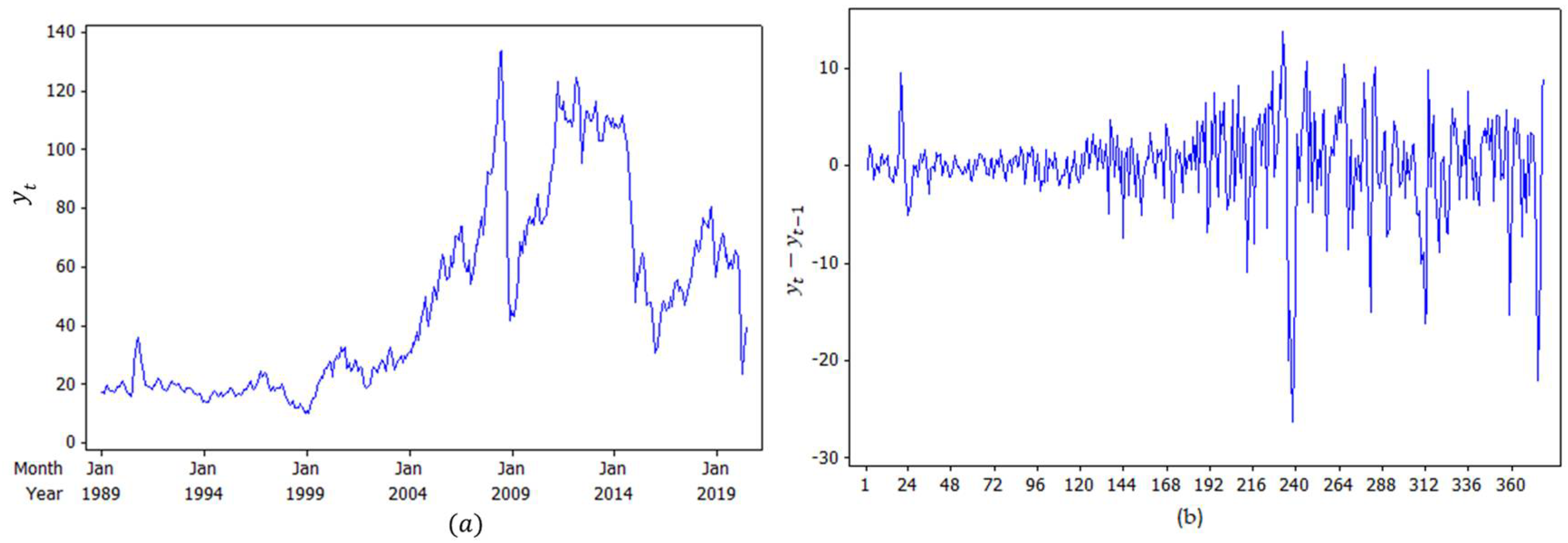
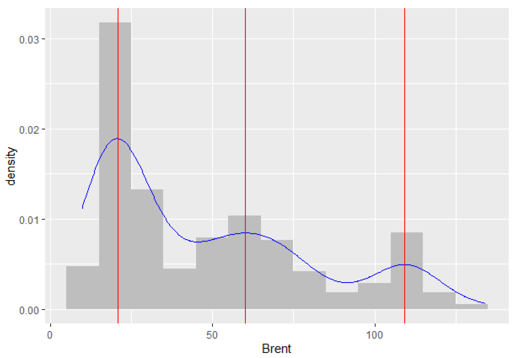
Section 5 contains the application and comparison of the models using the daily IBM stock prices and the monthly Brent crude oil prices. The conclusion and discussion are given in Section 6.

2. Four-Parameter Fisher’s z Distribution

Let Y be a random variable distributed as an F distribution with d 1 and d 2   degrees of freedom. The density of Z = 1 2 ln Y can be defined as
ζ ( d 1 k , d 2 k ) ( z ) = f Z ( z ; d 1 , d 2 ) = 2 ( d 2 d 1 ) 1 2 d 2 B ( 1 2 d 1 , 1 2 d 2 ) e d 2 z ( 1 + e 2 z + ln d 2 d 1 ) ( d 1 + d 2 ) / 2 ,
and the cumulative distribution function (CDF) of Z is expressed as
Z ( d 1 k , d 2 k ) ( z ) = I z * ( 1 2 d 2 , 1 2 d 1 ) = 0 z * t 1 2 d 2 1 ( 1 t ) 1 2 d 1 1 d t B ( 1 2 d 1 , 1 2 d 2 ) ,
where e is the exponential constant; z * = d 2 e 2 z d 1 + d 2 e 2 z ,   I z * ( . ) is the incomplete beta function ratio; and B ( . ) is the beta function, < z < ,   d 1 > 0 ,   d 2 > 0 . Equations (1) and (2) are defined as a probability density function (p.d.f) and a CDF of standardized Fisher’s z distribution, respectively. Let Z be a random variable distributed as a standardized Fisher’s z distribution. Let μ be a location parameter, and let σ be a scale parameter. The density of X = σ Z + μ is (Solikhah et al. 2021)
f X ( x ; d 1 , d 2 , μ , σ ) = 2 σ ( d 2 d 1 ) 1 2 d 2 B ( 1 2 d 1 , 1 2 d 2 ) e d 2 ( x μ σ ) ( 1 + e 2 ( x μ σ ) + ln d 2 d 1 ) ( d 1 + d 2 ) / 2 ,
where < x < , < μ < ,   and σ > 0 . Equation (3) is defined as a p.d.f of Fisher’s z distribution. It is denoted as z ( d 1 , d 2 , μ , σ ) . The CDF of the Fisher’s z distribution is expressed as
F X ( x ; d 1 , d 2 , μ , σ ) = I x * ( 1 2 d 2 , 1 2 d 1 ) = 1 B ( 1 2 d 1 , 1 2 d 2 ) 0 x * t 1 2 d 2 1 ( 1 t ) 1 2 d 1 1 d t ,
where x * = d 2 e 2 ( x μ σ ) d 1 + d 2 e 2 ( x μ σ )   . The quantile function (QF) of the Fisher’s z distribution is defined as
x p = μ + σ 2 ln d 2 I 1 x p ( 1 2 d 1 , 1 2 d 2 ) d 1 ( 1 I 1 x p ( 1 2 d 1 , 1 2 d 2 ) ) ,
where ( d 2 I 1 x p ( 1 2 d 1 , 1 2 d 2 ) ) / ( d 1 ( 1 I 1 x p ( 1 2 d 1 , 1 2 d 2 ) ) ) is the QF of the F-distribution and I 1 x p ( . ) is the inversion of the incomplete beta function ratio. Let P 1 x p ( . ) be the inversion of the incomplete gamma function ratio. The QF of the Fisher’s z distribution can be expressed as
x p = μ + σ 2 ln ( d 2 ( P 1 v 1 p ( d 1 / 2 ) ) d 1 ( P 1 v 2 p ( d 2 / 2 ) ) )   ,
where 2   P 1 v 1 p ( 1 2 d 1 ) and 2   P 1 v 2 p ( 1 2 d 2 ) are the QF of the chi-square distribution with d 1 and d 2 degrees of freedom, respectively. The proofs of Equation (1) up to Equation (6) are postponed to Appendix A. The parameters d 1 and d 2 , known as the shape parameters, are defined for both skewness (symmetrical if d 1 = d 2 , asymmetrical if d 1 d 2 ) and fatness of the tails (large d 1 and d 2 imply thin tails). The Fisher’s z distribution is also always unimodal and has the mode at x = μ . Furthermore, a change in the value of the parameter μ only affects the mean of the distribution. It does not affect the variance, skewness, and kurtosis of the distribution. The detailed properties of the Fisher’s z distribution are shown in Appendix B.
A useful tutorial on adding custom function to Stan is provided by Stan Development Team (2018) and Annis et al. (2017). To add a user-defined function, it is first necessary to define a block of function code. The function block must precede all other blocks of Stan code. The code for the random numbers generator function (fisher_z_rng) is shown in Appendix C.1, and the log probability function (fisher_z_lpdf) is shown in Appendix C.2. As an illustration, the p.d.f and CDF of the Fisher’s 
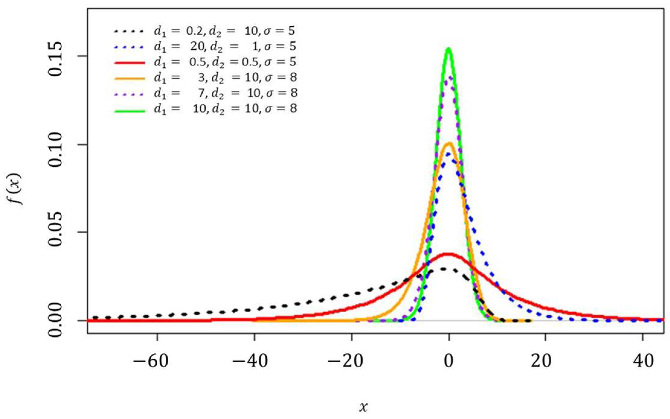
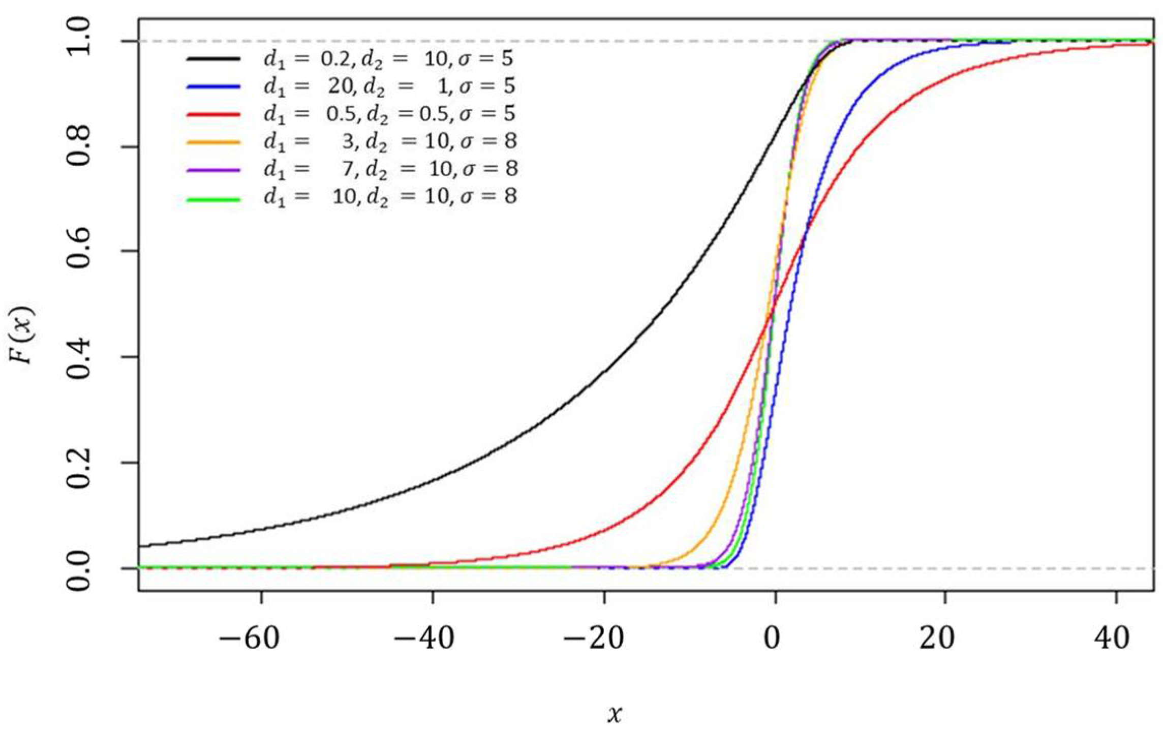
z distribution with various parameter settings can be seen in Figure 1 and Figure 2, respectively.

3. Fisher’s z Mixture Autoregressive Model

3.1. Model Specification

Let y t ;   t = 1 , 2 , , T   be the real-valued time series of interest; let ( t 1 ) denote the information set up to time t 1 , let F ( y t | ( t 1 ) ) ; k = 1 , 2 , , K be the conditional CDF of Y t given the past information, evaluated at y t ; and K is the number of components in the ZMAR model. Let Z ( d 1 k , d 2 k ) ( . ) be the CDF of the standardized Fisher’s z distribution with d 1 k   and d 2 k shape parameters, given by Equation (2); let ϵ k . t be a sequence of independent standardized Fisher’s z random variables such that ϵ k . t is independent of { y t i ,   i > 0 } ; and let σ k is a scale parameter of the kth component. The K -component ZMAR can be defined as
F ( y t | ( t 1 ) ) = k = 1 K η k Z ( d 1 k , d 2 k ) ( y t μ k . t σ k ) ,
or
y t = { μ 1 . t + σ 1 ϵ 1 . t ; with   probability   η 1 ; μ 2 . t + σ 2 ϵ 2 . t ; with   probability   η 2 ; μ K . t + σ K ϵ K . t ; with   probability   η K ,
with
μ k . t = ϕ k . 0 + i = 1 p k ϕ k . i y t i   ; k = 1 , 2 , , K   ,
where the vector η = ( η 1 ,   .   .   .   , η K ) is called the weights. η takes a value in the unit simplex K , which is a subspace of ( + ) K , defined by the following constraint, η k > 0 and k = 1 K η k = 1 . We use the abbreviation ZMAR ( K ; p 1 ,   p 2 , ,   p K ) for this model, with the parameter ϑ = ( θ 1 , θ 2 , ,   θ K , η ) ; η = ( η k ) ; θ k = ( d 1 k , d 2 k , σ k , ϕ k . 0 , ϕ k ) ; ϕ k = ( ϕ k . 1 , ϕ k . 2 ,   , ϕ k . p k ) ; to each value k { 1 , 2 ,   .   .   .   , K } ; taking values in the parameter space Θ K = Θ K × K , ϕ k . i denotes the AR coefficient on the kth component and ith lag; i = 1 , 2 ,   ,   p k ; and p k denotes the autoregressive order of the kth component. Using the parameters θ k , we first define the K auxiliary Fisher’s z AR( p k ) processes
f k ( y t | ( t 1 ) ) = ϕ k . 0 + i = 1 p k ϕ k . i y t i   + σ k ϵ k . t   ; k = 1 , 2 , , K ,
where the AR coefficients ϕ k are assumed to satisfy
1 i = 1 p k ϕ k . i C i 0   for   | C | 1 ; k = 1 , , K .
This condition implies that the processes f k ( y t | ( t 1 ) ) are stationary and that each component model in (7) or (8) satisfies the usual stationarity condition of the linear AR( p k ) model.
Suppose p = max ( p 1 , p 2 ,   .   .   .   ,   p K ) . Let a univariate time series y = ( y 1 , y 2 , , y T ) be influenced by a hidden discrete indicator variables Q = ( Q 1 , Q 2 , , Q T ) , where Q t takes values in the set { 1 , 2 , , K } . The probability of sampling from the group labeled Q t = k is equal to η k . Suppose that the conditional density of Y t given Q t = k is f k ( y t | ( t 1 ) ) ; ( k = 1 , 2 ,     ,   K ) .   Let H = ( H 1 , H 2 ,   .   .   .   ,   H T ) be the unobserved random variable, where H t is a K -dimensional vector with the values h = ( h 1 , h 2 ,   .   .   .   ,   h T ) , where h k . t = 1 if Q t = k and h k . t = 0 , otherwise. Thus, H t is distributed according to a multinomial distribution consisting of one draw on K categories with probabilities η 1 ,   η 2 ,   ,   η K (McLachlan and Peel 2000, p. 7); that is,
P ( H t = h t ) = η 1 h 1 . t   η 2 h 2 . t η K h K . t   .
Otherwise, this can be written as H t ~ Mult K ( 1 , η ) ; where η = ( η 1 ,   η 2 ,   .   .   .   , η K ) . The conditional likelihood for the ZMAR ( K ;   p 1 ,   p 2 , ,   p K ) can be formed by
P ( y t | ϑ ) = k = 1 K t = p + 1 T [ η k Δ 1 Δ 2 ] h k . t ,
where Δ 1 = 2 (   d 2 k / d 1 k ) 1 2   d 2 k σ k B ( 1 2 d 1 k , 1 2   d 2 k ) ,   Δ 2 = exp ( d 2 k ( a k . t / σ k ) ) [ 1 + exp ( 2 ( a k . t / σ k ) + ln [ d 2 k / d 1 k ] ) ] ( d 1 k + d 2 k ) / 2 , and a k . t = y t μ k . t .
Let τ t . k be the probability for each t-th observation, t = ( p + 1 ) , ( p + 2 ) , , T , as members of the k-th component, k = 1 , 2 , , K of a mixture distribution. Suppose y t = ( y 1 , y 2 , , y t ) , Bayes’ rule to compute the τ t . k can be expressed as (Frühwirth-Schnatter 2006, p. 26)
P ( Q t = k | y t , ϑ ) = τ t . k = η k f k ( y t | ( t 1 ) ) k = 1 K η k f k ( y t | ( t 1 ) ) .
Let ζ ( d 1 k , d 2 k ) ( . ) be the p.d.f of the standardized Fisher’s z distribution and given by Equation (1). Then, the mixing weights for the ZMAR model can be expressed as
τ t . k = η k σ k 1 ζ ( d 1 k , d 2 k ) ( a k . t / σ k ) k = 1 K η k σ k 1 ζ ( d 1 k , d 2 k ) ( a k . t / σ k ) ; k = 1 , 2 , , K .
Suppose ω k . t and ξ k 2 signify the conditional mean and conditional variance of the kth component, which are defined by
ω k . t = E [ Y t |   θ k ] = μ k . t + σ k 2 ( ln d 2 k d 1 k ψ ( 1 2 d 2 k ) + ψ ( 1 2 d 1 k ) ) ,
and
ξ k 2 = Var [ Y t |   θ k ] = ( σ k 2 ) 2 ( ψ ( 1 2 d 2 k ) + ψ ( 1 2 d 1 k ) ) ,
where ψ ( . ) is the digamma function and ψ ( . ) is the trigamma function. The conditional mean of Y t (Frühwirth-Schnatter 2006, p. 10) is obtained as
ω t = E [ Y t | ( t 1 ) ] = k = 1 K η k ω k . t ,
the conditional variance of Y t (Frühwirth-Schnatter 2006, p. 11) is obtained as
ξ 2 = Var [ Y t | ( t 1 ) ] = k = 1 K η k ( ω k . t 2 + ξ k 2 ) ω t 2 ,
and the higher-order moments around the mean of Y t (Frühwirth-Schnatter 2006, p. 11) are obtained as
E ( ( Y ω t ) 3 | ( t 1 ) ) = k = 1 K ( ( ω k . t ω t ) 2 + 3 ξ k 2 ) ( ω k . t ω t ) η k ,
E ( ( Y ω t ) 4 | ( t 1 ) ) = k = 1 K ( ( ω k . t ω t ) 4 + 6 ( ω k . t ω t ) 2 ξ k 2 + 3 ξ k 4 ) η k .
These expressions apply to any specification of the mixing weights η k .

3.2. Bayesian Approach for ZMAR Model

In this paper, we apply a Bayesian method to estimate the parameters ϑ . The Bayesian analysis requires the joint posterior density π ( ϑ | y ) , which is defined by
π ( ϑ | y ) P ( y t | ϑ ) π ( ϑ ) ,
where P ( y t | ϑ ) is the conditional likelihood function given by Equation (11) and π ( ϑ ) is the prior of the parameter model, which is defined by
π ( ϑ ) = π ( η ) k = 1 K π ( d 1 k ) π ( d 2 k ) π ( σ k ) π ( ϕ k . 0 ) i = 1 p k π ( ϕ k . i ) ,
where the π ( η ) is prior for the η parameter, the π ( d 1 k ) ,   π ( d 2 k ) ,   π ( σ k ) ,   π ( ϕ k . 0 ) and π ( ϕ k . i )   are prior for the d 1 ,   d 2 ,   σ ,   ϕ 0 and ϕ i parameters at the kth component; index i denotes the ith lag; i = 1 , 2 , , p k ; k = 1 , 2 , , K .
Various noninformative prior distributions have been suggested for the prior of AR coefficients, scale parameters, and the selection probabilities in similar models. Huerta and West (1999) analyzed and used the uniform Dirichlet distribution as the prior distribution for the latent variables related to the latent components of an autoregressive model. Gelman (2006) suggested working within the half-t family of prior distributions for variance parameters in the hierarchical modelling, which are more flexible and have better behavior near 0, compared to the inverse-gamma family. Albert and Chib (1993) used the normal distribution as the prior for the autoregressive coefficient in the Markov switching autoregressive model. Based on the findings of the previous studies, we take the singly truncated Student t distribution (positive values only) (Kim 2008) for the priors of the d 1 k ,     d 2 k , and σ k , with the degrees of freedoms v 1 k ,   v 2 k , ν 3 k , the location parameters m 1 k , m 2 k , m 3 k , and the scale parameters s 1 k 2 ,   s 2 k 2 , s 3 k 2 , respectively. Therefore, it can be written as d 1 k ~   t ν 1 k ( m 1 k , s 1 k 2 ) I ( 0 , ) ,   d 2 k ~   t ν 2 k ( m 2 k , s 2 k 2 ) I ( 0 , ) ,   and σ k ~   t ν 3 k ( m 3 k , s 3 k 2 ) I ( 0 , ) . We take the Dirichlet distribution (Kotz et al. 2000, p. 485) for the prior of the η parameter, thus η 1 , η 2 , , η K 1   ~   Dir ( δ 1 , δ 2 , , δ K ) . For the priors of the ϕ k . 0 and ϕ k . i , we take the normal distribution with the location parameters u k . 0 ,   u k . i and the scale parameters g k . 0 2 ,   g k . i 2 , thus ϕ k . 0 ~ N ( u k . 0 , g k . 0 2 ) and ϕ k . i ~ N ( u k . i , g k . i 2 ) ; i = 1 , 2 , , p k . Employing the setup of prior distributions, as shown above, the natural logarithm of the joint posterior distribution of the model is given by
ln π ( ϑ | y ) k = 1 K ( ( t = p + 1 T h k . t ( ln η k + Λ 1 + Λ 2 ) ) + Λ 3 + Λ 4 + Λ 5 + Λ 6 + Λ 7 + i = 1 p k Λ 8 ) ,
where Λ 1 = d 2 k ln [ d 2 k / d 1 k ] + ln [ Γ ( 1 2 (   d 1 k + d 2 k ) ) ] ln [ Γ ( 1 2   d 1 k ) ] ln [ Γ ( 1 2   d 2 k ) ] ln σ k , Λ 2 =   d 2 k ( a k . t σ k ) d 1 k +   d 2 k 2 ln [ 1 + exp [ 2 a k . t σ k + ln [ d 2 k / d 1 k ] ] ] ,   Λ 3 = ( δ K 1 ) ln [ 1 k = 1 K 1 η k ] + k = 1 K 1 ( δ k 1 ) ln η k , Λ 4 = 1 2 ( ν 1 k + 1 ) ln [ 1 + 1 ν 1 k ( d 1 k m 1 k s 1 k ) 2 ] ,   Λ 5 = 1 2 ( ν 2 k + 1 ) ln [ 1 + 1 ν 2 k ( d 2 k m 2 k s 2 k ) 2 ] , Λ 6 = 1 2 ( ν 3 k + 1 ) ln [ 1 + 1 ν 3 k ( σ k m 3 k s 3 k ) 2 ] , Λ 7 = 1 2 ( ϕ k . 0 u k . 0 g k . 0 ) 2 , and Λ 8 = 1 2 ( ϕ k . i u k . i g k . i ) 2 .
HMC requires the gradient of the ln-posterior density. In practice, the gradient must be computed analytically (Gelman et al. 2014, p. 301). The gradient of ( ϑ | y ) is
ϑ ( ϑ | y ) = ϑ ln π ( ϑ | y )
ϑ ( ϑ | y ) = ( ( ϑ | y ) η k , ( ϑ | y ) d 1 k , ( ϑ | y ) d 2 k , ( ϑ | y ) σ k , ( ϑ | y ) ϕ k . 0 , ( ϑ | y ) ϕ k . i )
where i = 1 , 2 , , p k ; k = 1 , 2 , , K . The HMC algorithm for estimating the parameters of the ZMAR model is as follows:
  • Determine the initial value of the parameter ϑ 0 , the diagonal mass matrix M , the scale factor of the leapfrog steps ε , the number of leapfrog steps N , and the number of iterations .
  • For each iteration r ; r = 1 , 2 , , where represents the number of iterations,
    • Generate the momentum variables φ with φ ~ Normal ( 0 , M ) ;
    • For each iteration n = 1 , 2 , , N ,
      (1)
      Use the gradient of the ln-posterior density of ϑ n to make a half-step of φ n
      φ n + 0.5 φ n + 1 2 ε ln π ( ϑ n | y ) ϑ n ,
      (2)
      Update the vector ϑ n using the vector φ n + 0.5
      ϑ n + 0.5 ϑ n + ε M 1 φ n + 0.5
      (3)
      Update the next half-step for φ
      φ n + 1 φ n + 0.5 + 1 2 ε ln π ( ϑ n + 0.5 | y ) ϑ n + 0.5 .
    • Labels ϑ ( r 1 ) and φ ( r 1 ) as the value of the parameter and momentum vectors at the start of the leapfrog process and ϑ # ,   φ # as the value after the N steps.
    • Compute
      b = π ( ϑ # | y ) f ( φ # ) π ( ϑ ( r 1 ) | y ) f ( φ ( r 1 ) )   .
    • Set ϑ ( r )
      ϑ ( r ) = { ϑ #   with   probability   m i n ( b , 1 )   ϑ ( r 1 )   otherwise .  
    • Save ϑ ( r ) ;   r = 1 , 2 , , .
The performance of the HMC is very sensitive to two user-defined parameters, i.e., the step size of the leapfrog ε and the number of leapfrog steps L . The No-U-Turn Sampler (NUTS) could eliminate the need to set the parameter L and could adapt the step size parameter ε on the fly based on a primal-dual averaging (Hoffman and Gelman 2014). The NUTS algorithm was implemented in C ++ as part of the open-source Bayesian inference package, Stan (Gelman et al. 2014, p. 304; Carpenter et al. 2017). Stan is also a platform for computing log densities and their gradients, so that the densities and gradients are easy to obtain (Carpenter et al. 2015, 2017). Stan can be called from R using the rstan package. An example of the Stan code to fit the ZMAR model can be seen in Section 4.

4. Simulation Studies

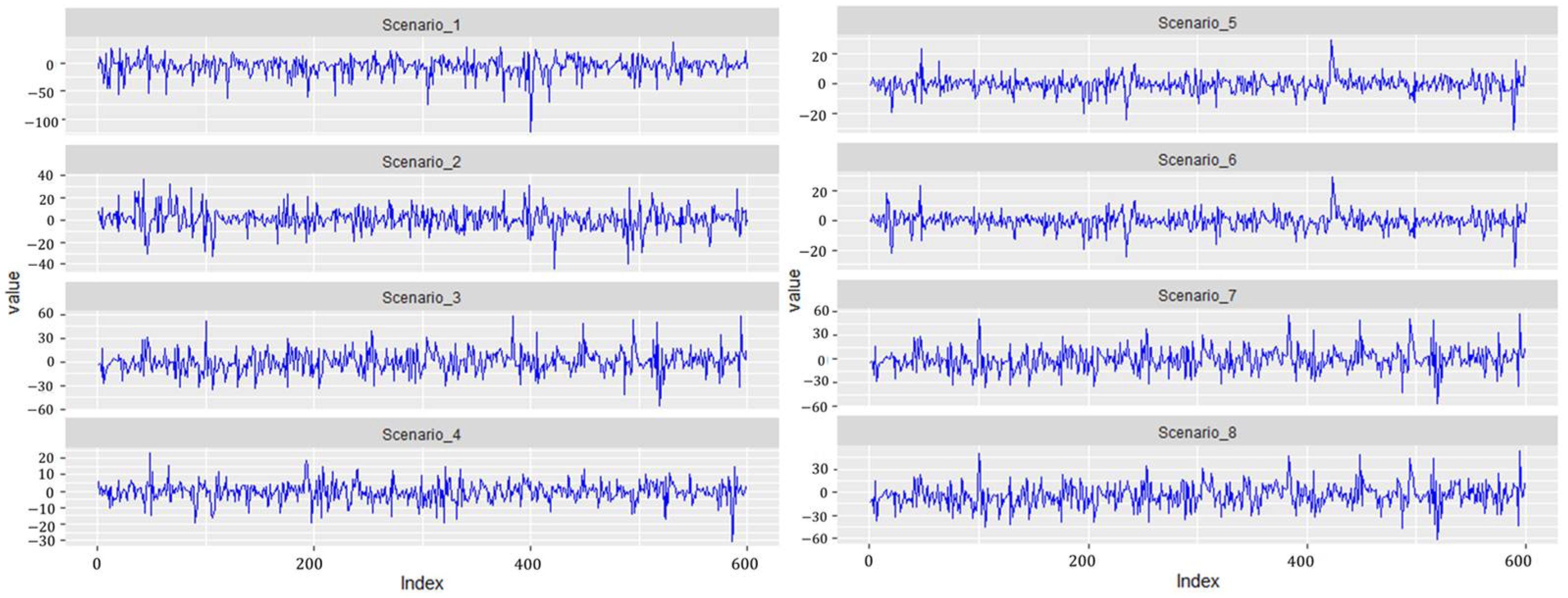
A simulation study was carried out to evaluate the performance of the ZMAR model compared to the TMAR and GMAR models. We consider the simulations to accommodate eight scenarios for the conditional density in the first component of the ZMAR model. Furthermore, the conditional densities in the second and third components are specified as the symmetric-fat-tail of the Fisher’s z distributions.
We conducted a Bayesian analysis on the eight simulated datasets, whose datasets were generated by the following steps:
  • Step 1: Specify the ZMAR model with three components as ZMAR ( 3 ; 1 , 1 , 1 ) where f ( y t | ( t 1 ) ) = k = 1 3 η k f k ( y t | ( t 1 ) ) = k = 1 3 η k ( ϕ k . 0 + ϕ k . 1 y t 1   + e k . t ) ; η 1 = η 2 = η 3 = 1 3 ; ϕ 1.1 = 0.6 ;   ϕ 2.1 = 0.2 ; ϕ 3.1 = 0.7 with e k . t ~ z ( d 1 . k , d 2 . k , 0 , σ k ) ; k = 1 , 2 , 3 are the innovations in the first, second, and third components. The scenarios for the simulation are as follows:
    Scenario 1: represent a mixture of a highly skewed (Bulmer 1967, p. 63) to the left and two symmetrical distributions, where ϕ 1.0 = ϕ 2.0 = ϕ 3.0 = 0 , excess unconditional kurtosis is 5.73, e 1 . t ~ z ( 0.2 ,   10 ,   0 ,   5 ) ,   e 2 . t ~ z ( 1 ,   1 ,   0 ,   8 ) , and e 3 . t ~ z ( 30 ,   30 ,   0 ,   10 ) ;
    Scenario 2: represent a mixture of a highly skewed to the right and two symmetrical distributions, where ϕ 1.0 = ϕ 2.0 = ϕ 3.0 = 0 , excess unconditional kurtosis is 2.23, e 1 . t ~ z ( 20 ,   1 ,   0 ,   5 ) ,   e 2 . t ~ z ( 1 ,   1 ,   0 ,   8 ) , and e 3 . t ~ z ( 30 ,   30 ,   0 ,   10 ) ;
    Scenario 3: represent a mixture of three symmetrical distributions, where ϕ 1.0 = ϕ 2.0 = ϕ 3.0 = 0 , excess unconditional kurtosis is 1.67, e 1 . t ~ z ( 0.5 ,   0.5 ,   0 ,   5 ) , e 2 . t ~ z ( 1 ,   1 ,   0 ,   8 ) , and e 3 . t ~ z ( 30 ,   30 ,   0 ,   10 ) ;
    Scenario 4: represent a mixture of moderately skewed (Bulmer 1967, p. 63) distributions, where ϕ 1.0 = ϕ 2.0 = ϕ 3.0 = 0 , excess unconditional kurtosis is 2.12, e 1 . t ~ z ( 3 ,   10 ,   0 ,   8 ) ,   e 2 . t ~ z ( 1 ,   1 ,   0 ,   5 ) , and e 3 . t ~ z ( 30 ,   30 ,   0 ,   10 ) ;
    Scenario 5: represent a mixture of three fairly symmetrical distributions (Bulmer 1967, p. 63), where ϕ 1.0 = ϕ 2.0 = ϕ 3.0 = 0 , excess unconditional kurtosis is 4.25, e 1 . t ~ z ( 7 ,   10 ,   0 ,   8 ) ,   e 2 . t ~ z ( 1 ,   1 ,   0 ,   5 ) , and e 3 . t ~ z ( 30 ,   30 ,   0 ,   10 ) ;
    Scenario 6: represent a mixture of three symmetrical distributions, where ϕ 1.0 = ϕ 2.0 = ϕ 3.0 = 0 , excess unconditional kurtosis is 4.47, e 1 . t ~ z ( 10 ,   10 ,   0 ,   8 ) , e 2 . t ~ z ( 1 ,   1 ,   0 ,   5 ) , and e 3 . t ~ z ( 30 ,   30 ,   0 ,   10 ) ;
    Scenario 7: represent a mixture of three symmetrical distributions, where ϕ 1.0 = 1 ,   ϕ 2.0 = ϕ 3.0 = 0 , excess unconditional kurtosis is 1.63, e 1 . t ~ z ( 0.5 ,   0.5 ,   0 ,   5 ) , e 2 . t ~ z ( 1 ,   1 ,   0 ,   8 ) , and e 3 . t ~ z ( 30 ,   30 ,   0 ,   10 ) ;
    Scenario 8: represent a mixture of three symmetrical distributions, where ϕ 1.0 = 20 , ϕ 2.0 = ϕ 3.0 = 0 , excess unconditional kurtosis is 0.67, e 1 . t ~ z ( 0.5 ,   0.5 ,   0 ,   5 ) , e 2 . t ~ z ( 1 ,   1 ,   0 ,   8 ) , and e 3 . t ~ z ( 30 ,   30 ,   0 ,   10 ) ;
The innovations of Scenario 7 and Scenario 8 are the same as those of Scenario 3. The comparison of graph visualizations for the innovations in the first component in Scenario 1 to Scenario 6 represented specifically for the Fisher’s z distribution can be seen in Figure 1 and Figure 2;
  • Step 2: Generate e 1 . t , e 2 . t , and e 3 . t ;
  • Step 3: Generate H t ~ Mult 3 ( 1 , η ) ; where η = ( 1 3 ,   1 3 ,   1 3 ) ;
  • Step 4: Compute f k ( y t | ( t 1 ) ) = ϕ k . 0 + ϕ k . 1 y t 1   + e k . t ; k = 1 , 2 , 3;
  • Step 5: Compute y t = f 1 ( y t | ( t 1 ) ) h 1 . t f 2 ( y t | ( t 1 ) ) h 2 . t f 3 ( y t | ( t 1 ) ) h 3 . t .
Furthermore, we generated 600 datasets and fit all of the models for each simulated dataset, respectively, to find the best performance in terms of model comparisons. Figure 3 shows the simulated datasets for Scenario 1 to Scenario 8. We implemented the models using the rstan package (Stan Development Team 2020), the R interface to Stan developed by the Stan Development Team in the R software. Suppose p k = p k ; con _ eta = c ( 1 , 1 , 1 ) ; tau [ t , k ] = τ t . k ; eta [ k ] = η k ; sigma [ k ] = σ k ; d 1 [ k ] = d 1 k ; d 2 [ k ] = d 2 k ; phi k [ 1 ] = ϕ k . 1 ; k = 1 , 2 , 3 . Here is an example of the Stan code to fit the ZMAR model in Scenario 1:
fitMAR1 = "
functions{
real fisher_z_lpdf(real x,real d1,real d2,real mu,real sigma){
return (log(2)+0.5*d2*(log(d2)-log(d1))-d2*(x-mu)/sigma-log(sigma)-lbeta(0.5*d1,0.5*d2)-
    (d1+d2)/2*log1p_exp((-2*(x-mu)/sigma)+log(d2)-log(d1)));
}
}
data {
int<lower=0> p1;
int<lower=0> p2;
int<lower=0> p3;
int T;
vector[T] y;
vector[3] con_eta;
}
parameters {
simplex[3] eta; //mixing proportions
vector<lower = 0>[3] sigma;
vector<lower = 0>[3] d1;
vector<lower = 0>[3] d2;
real phi1[p1];
real phi2[p2];
real phi3[p3];
}
model {
matrix[T,3] tau;
real lf[T];
eta ~ dirichlet(con_eta);
//priors
sigma[1] ~ student_t(3,5,0.1);
sigma[2] ~ student_t(3,8,0.1);
sigma[3] ~ student_t(3,10,0.1);
d1[1] ~ student_t(3,0.2,0.1);
d1[2] ~ student_t(3,1,0.1);
d1[3] ~ student_t(3,30,0.1);
d2[1] ~ student_t(3,10,0.1);
d2[2] ~ student_t(3,1,0.1);
d2[3] ~ student_t(3,30,0.1);
phi1[1] ~ normal(-0.6,0.1);
phi2[1] ~ normal(0.2,0.1);
phi3[1] ~ normal(0.7,0.1);
//ZMAR model
for(t in 1:T) {
if(t==1) {
tau[t,1] = log(eta[1])+fisher_z_lpdf(y[t]/sigma[1]|d1[1], d2[1],0,1)-log(sigma[1]);
tau[t,2] = log(eta[2])+fisher_z_lpdf(y[t]/sigma[2]|d1[2], d2[2],0,1)-log(sigma[2]);
tau[t,3] = log(eta[3])+fisher_z_lpdf(y[t]/sigma[3]|d1[3], d2[3],0,1)-log(sigma[3]);
} else {
real mu1 = 0;
real mu2 = 0;
real mu3 = 0;
for (i in 1:p1)
mu1 += phi1[i] * y[t-i];
for (i in 1:p2)
mu2 += phi2[i] * y[t-i];
for (i in 1:p3)
mu3 += phi3[i] * y[t-i];
tau[t,1] = log(eta[1])+fisher_z_lpdf((y[t]-mu1)/sigma[1]|d1[1],d2[1],0,1)-log(sigma[1]);
tau[t,2] = log(eta[2])+fisher_z_lpdf((y[t]-mu2)/sigma[2]|d1[2],d2[2],0,1)-log(sigma[2]);
tau[t,3] = log(eta[3])+fisher_z_lpdf((y[t]-mu3)/sigma[3]|d1[3],d2[3],0,1)-log(sigma[3]);
}
lf[t] = log_sum_exp(tau[t,]);
}
target += sum(lf);
} "
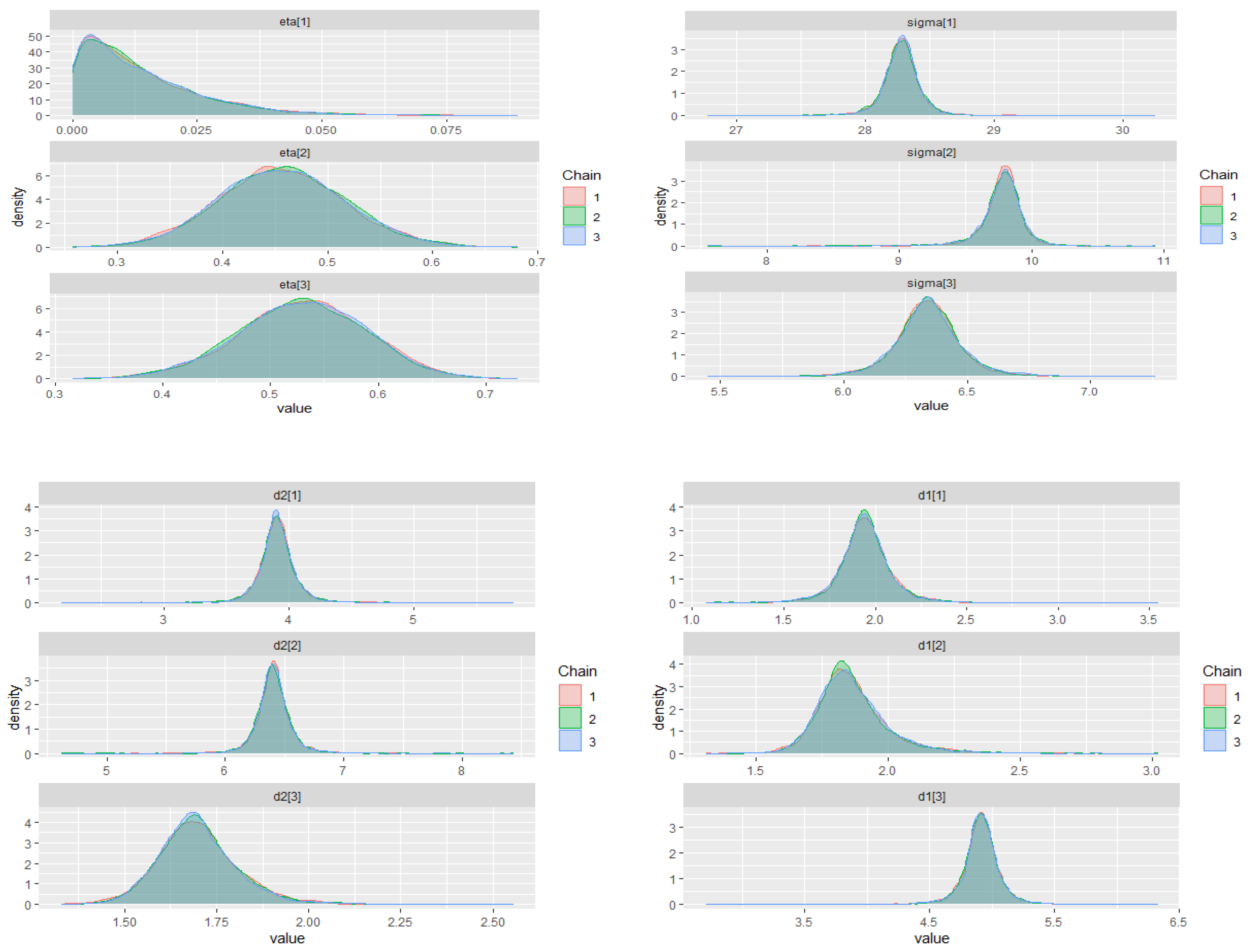
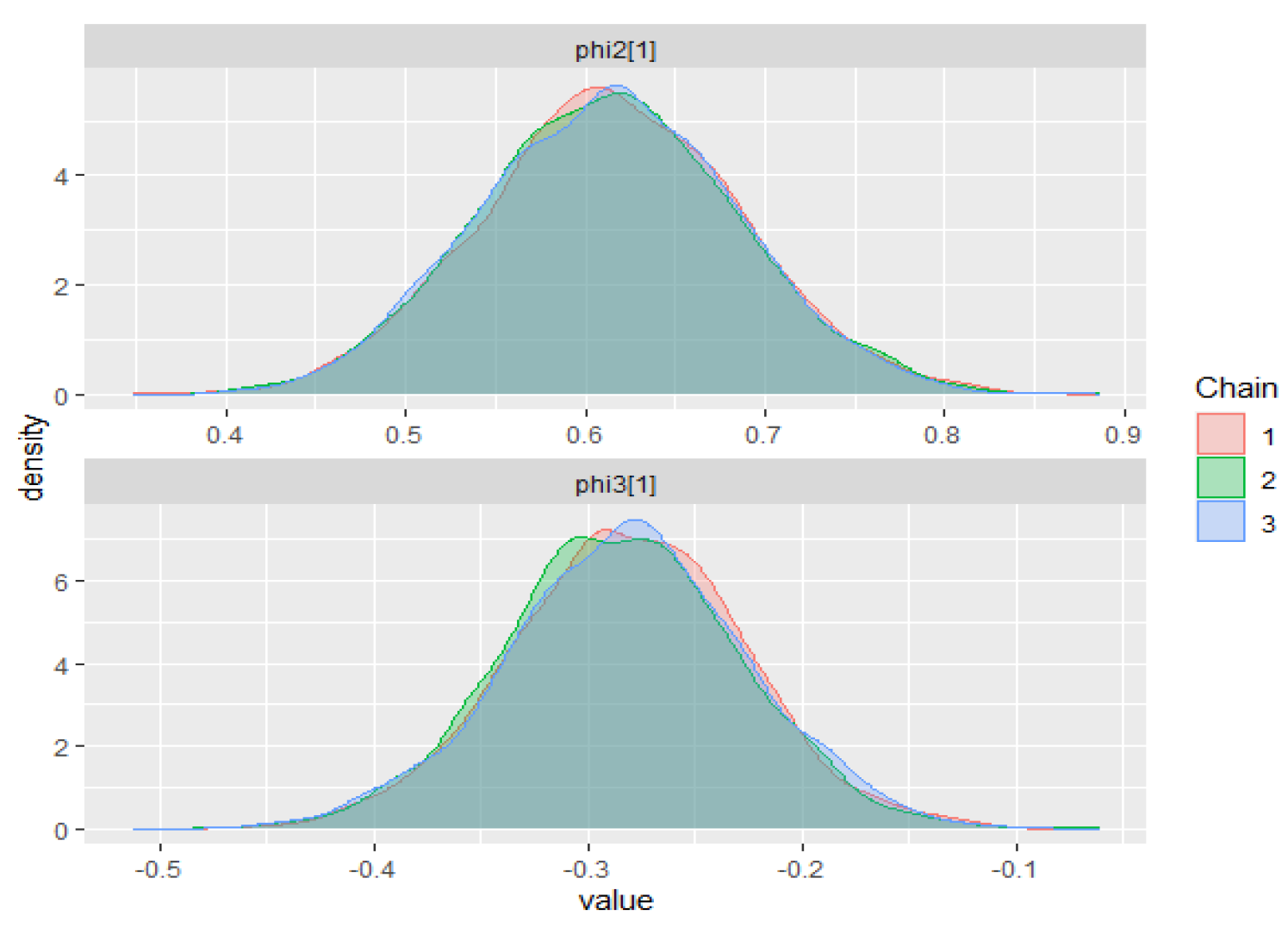
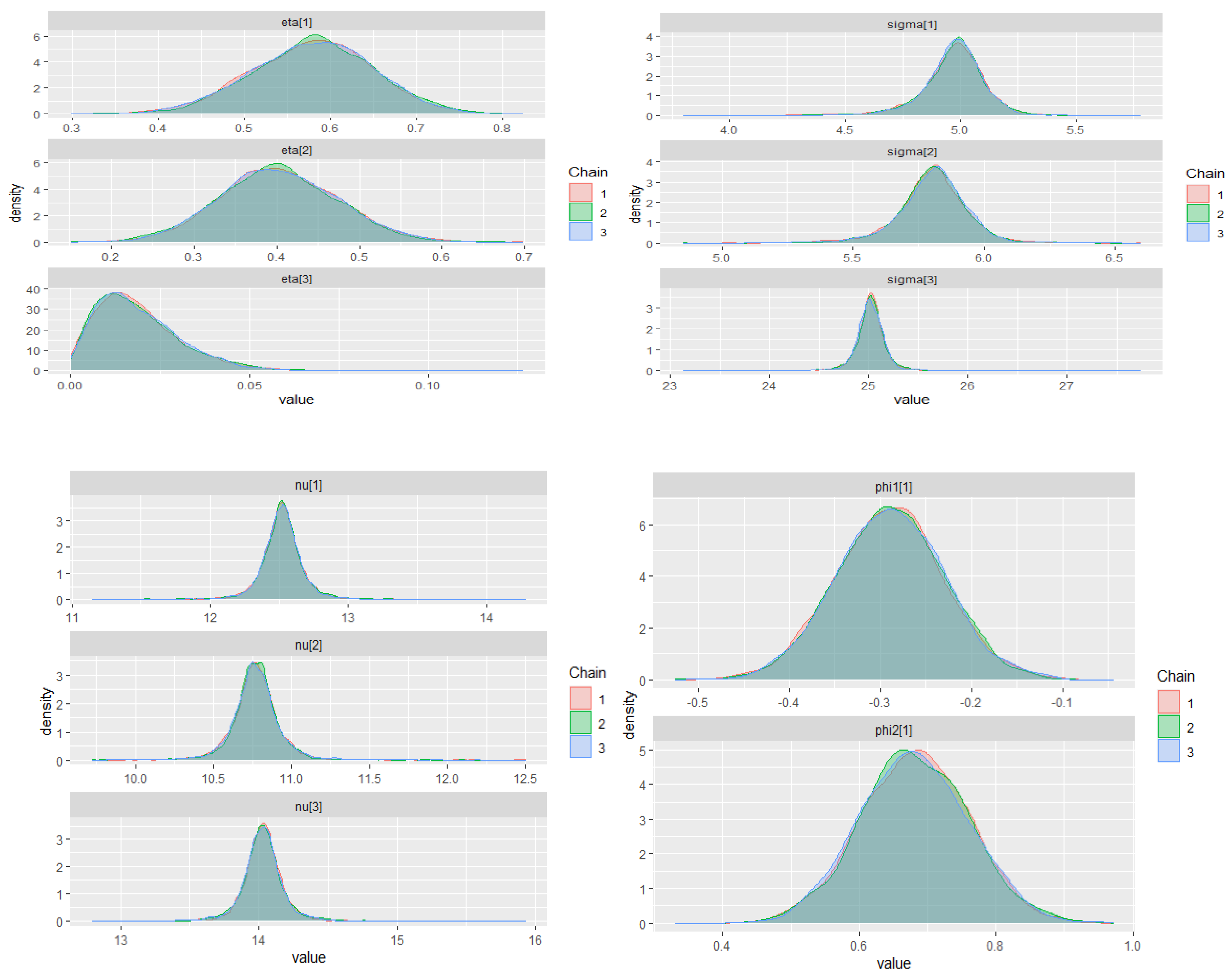
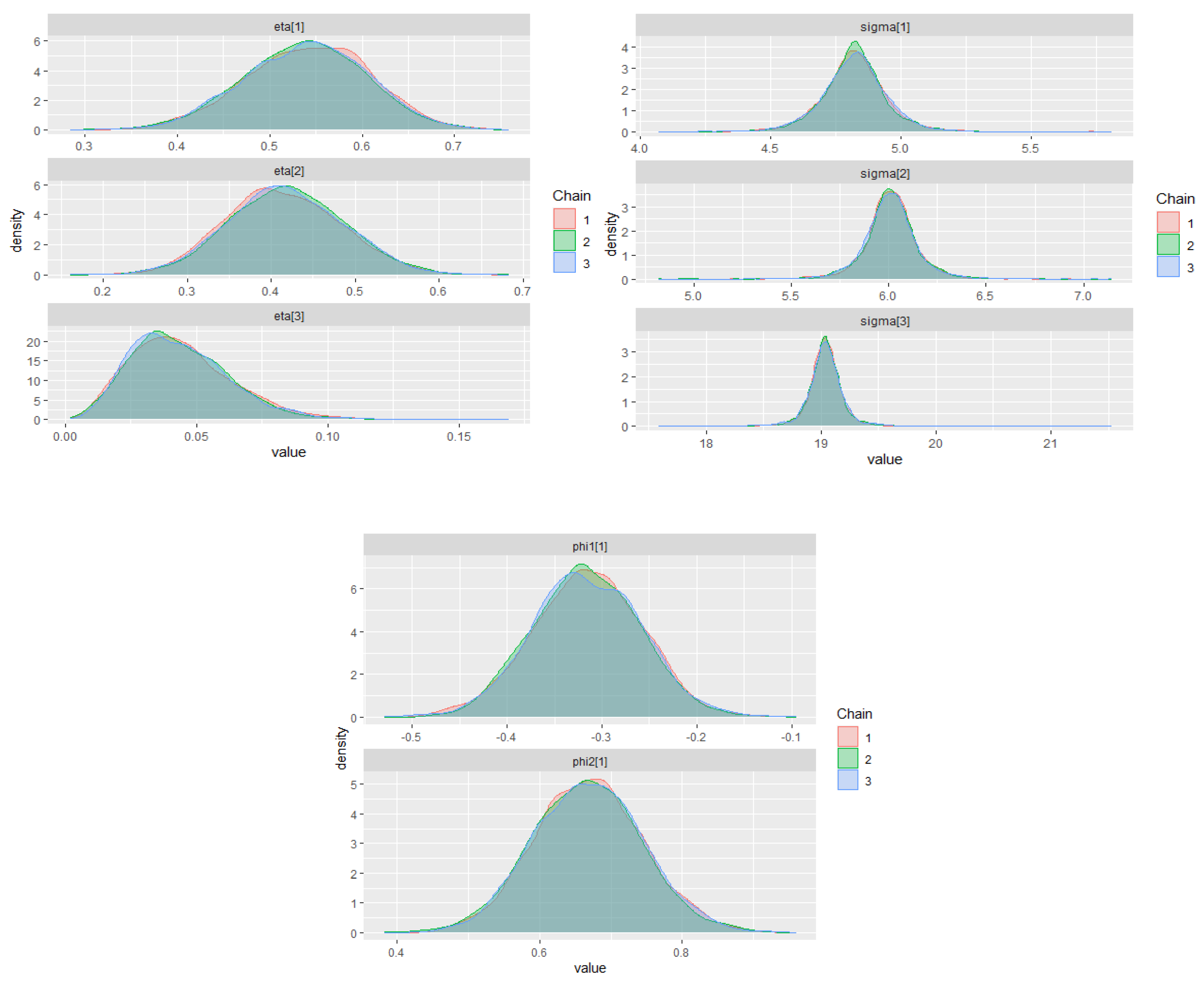
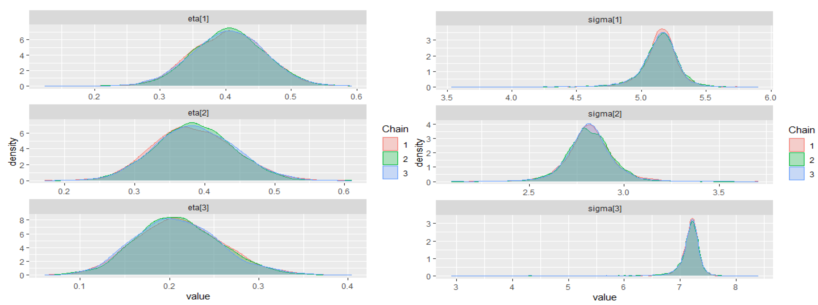
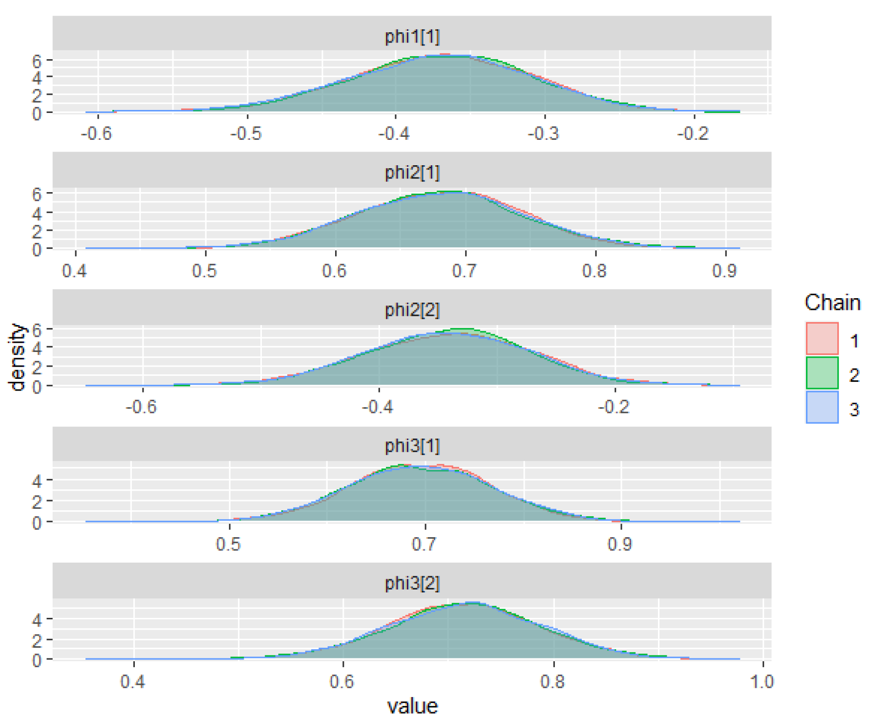
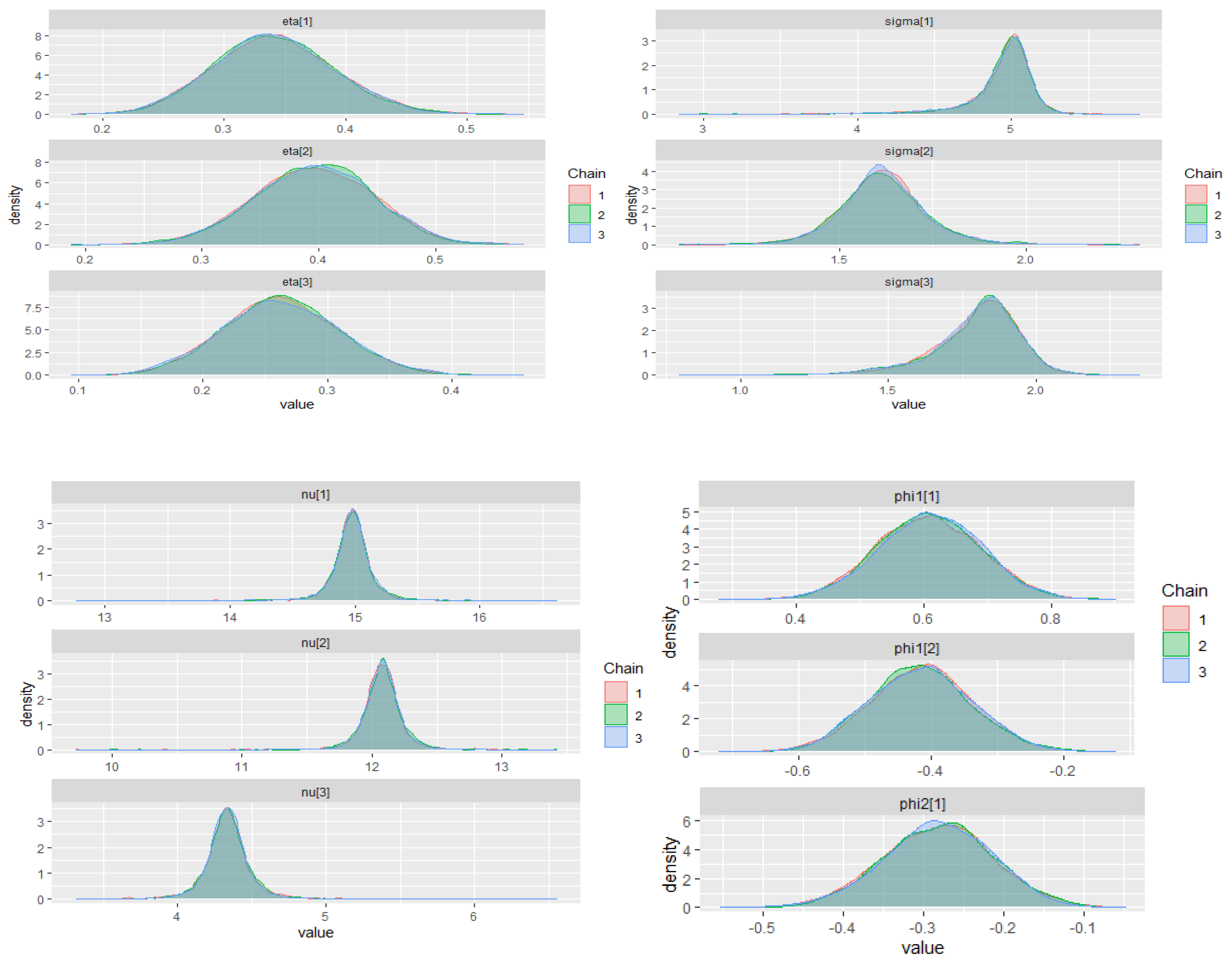
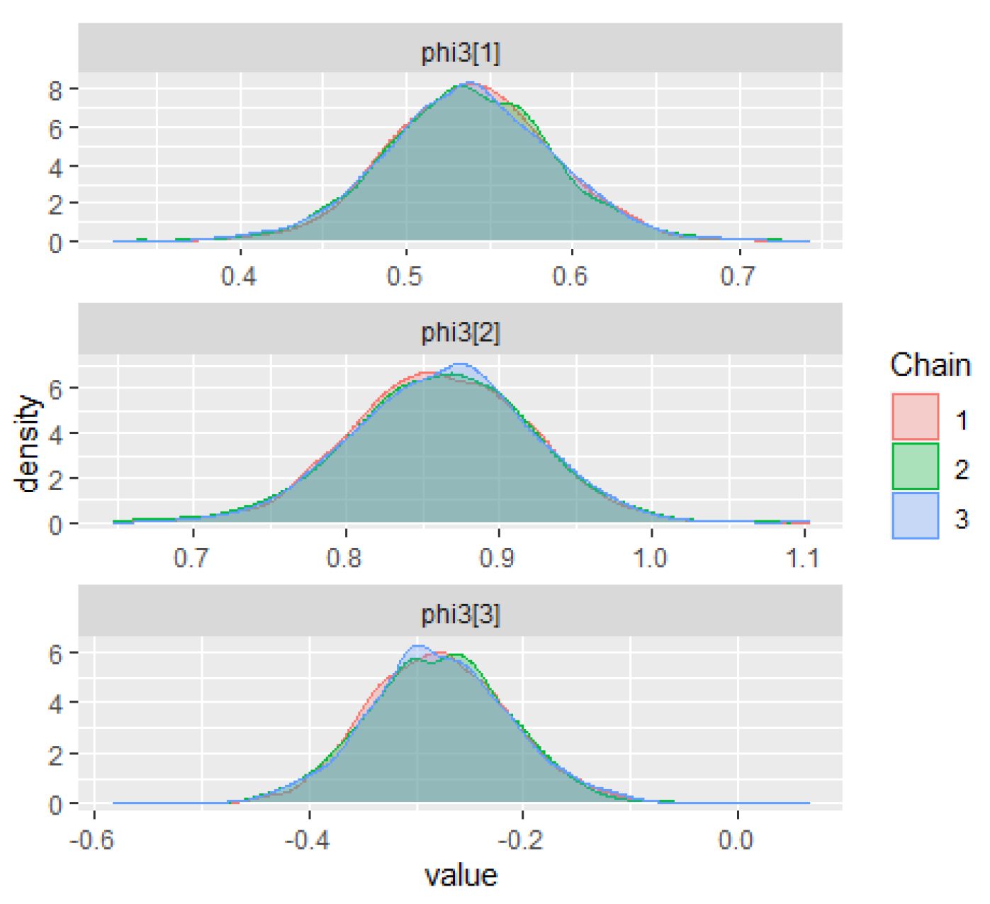
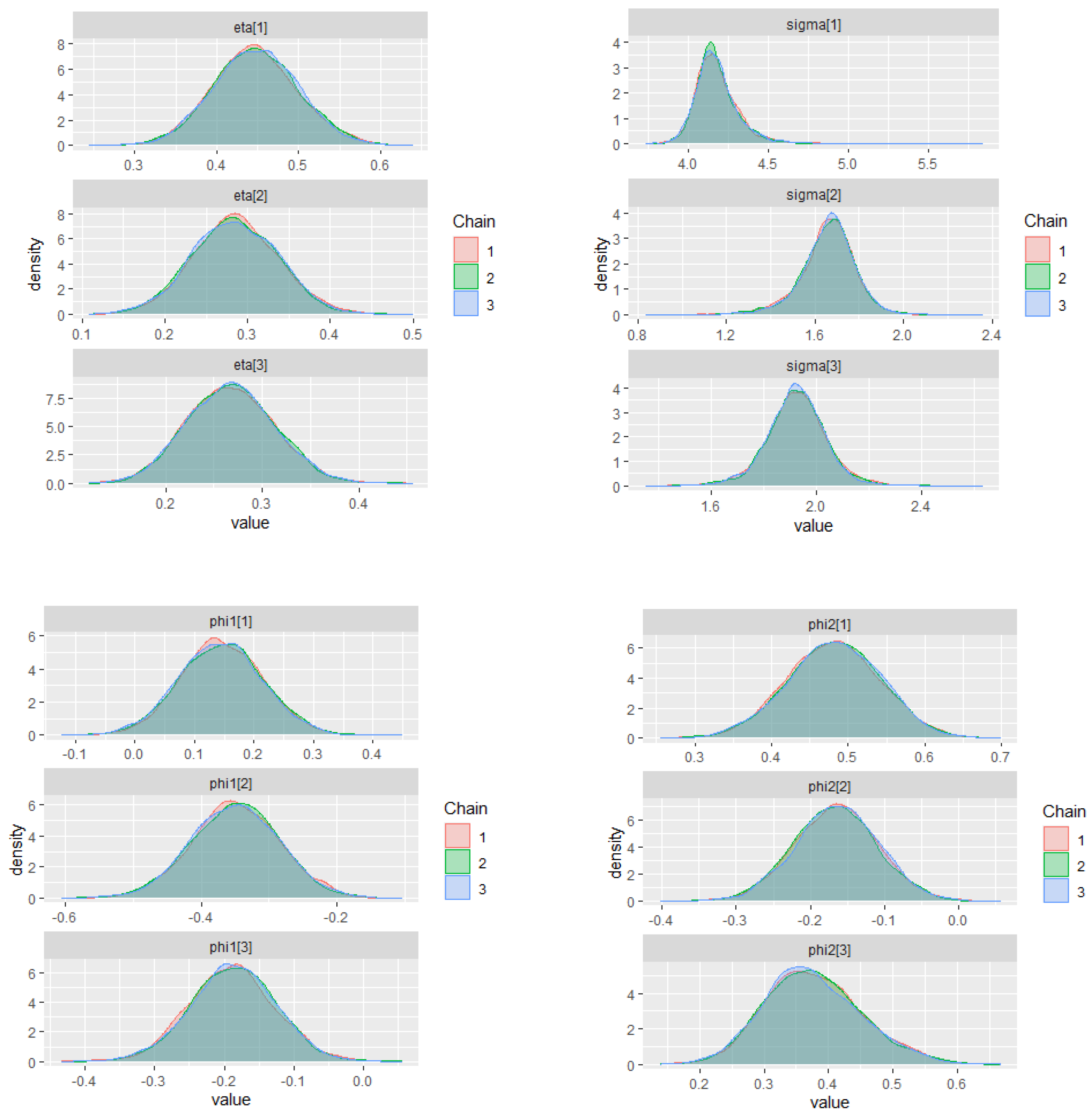
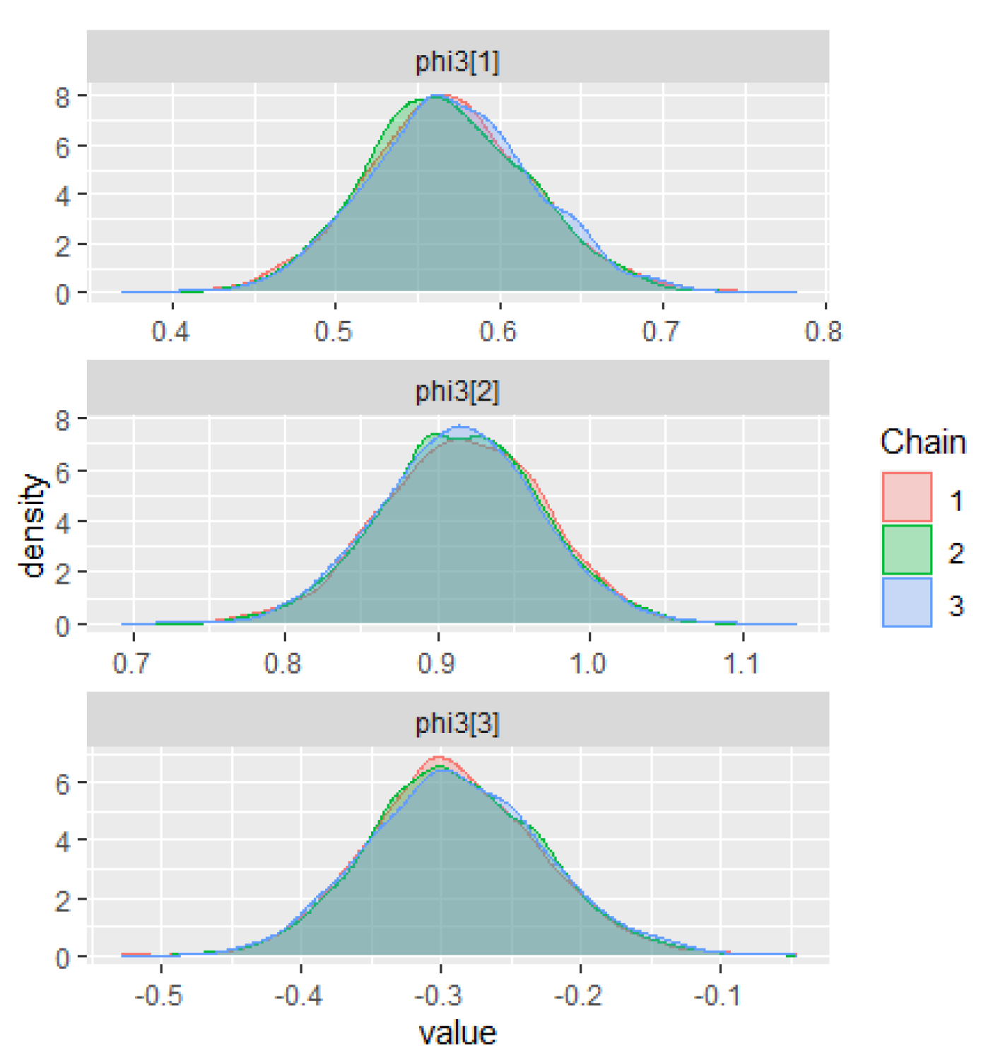
The warm-up stage in these simulation studies was set to 1500 iterations, 3 chains with 5000 sampling iterations, and 1 thin. The adapt_delta parameter was set to 0.99, and the max_treedepth was set to 15. For all scenarios, the parameter priors of the ZMAR, TMAR, and GMAR models are shown in Appendix D, and their posterior inferences are presented in Appendix E. There are a variety of convergence diagnoses, such as the potential scale reduction factor R ^ (Gelman and Rubin 1992; Susanto et al. 2018; Gelman et al. 2014, p. 285; Vehtari et al. 2020) and the effective sample size neff (Gelman et al. 2014, p. 266; Vehtari et al. 2020). If the MCMC chain has reached convergence, the R ^ statistic is less than 1.01, and the neff statistic is greater than 400 (Vehtari et al. 2020). To compare the performance of the models, we use the PSIS-LOO.
Table 1 shows the summary simulation result for all scenarios, which indicates that the ZMAR model performs the best when the datasets are generated from the ZMAR model, in which one of the components is asymmetric. When all the components are symmetric, the ZMAR model also performs better than TMAR and GMAR, as long as the excess unconditional kurtosis is large enough or the intercept distances between the components are far apart. However, when all of the mixture components are symmetric, the excess unconditional kurtosis is small and the intercept distances between the components are close enough or the intercepts are the same, then the GMAR model plays the best. Let us now focus on the results of Scenario 3 and Scenario 6.
In the third and sixth scenarios, the datasets are generated from three symmetrical distributions. The two scenarios have the same intercepts and are generated with different unconditional kurtosis. Scenario 3 has a smaller unconditional kurtosis than Scenario 6. The best ZMAR, TMAR, and GMAR models for the two scenarios are ZMAR(3;1,1,1), TMAR(3;1,1,1), and GMAR(3;1,1,1), where the values of PSIS-LOO are 4483.30, 4483.10, and 4481.10, for the third scenario and 3490.10, 3496.20, and 3494.60, for the sixth scenario. Clearly, the PSIS-LOO value for the GMAR model is smaller than for the ZMAR and TMAR models in the third scenario, and the ZMAR model has the smallest PSIS-LOO value in the sixth scenario. When the intercepts in Scenario 3 are varied and determined as in Scenario 7, the GMAR model is also the best. However, when the intercepts in Scenario 3 are varied and determined as in Scenario 8, the ZMAR model is the best. For other scenarios, in datasets generated from asymmetric components (the first, second, fourth, and fifth scenarios), the ZMAR model is the best.

5. Application for Real Data

5.1. IBM Stock Prices

To illustrate the potential of the ZMAR model, we consider the daily IBM common stock closing price from 17 May 1961 to 2 November 1962 (Box et al. 2015, p. 627). This time series has been analyzed by many researchers such as Le et al. (1996) and Wong and Li (2000). Wong and Li (2000) used the EM algorithm to estimate the parameters model and has been identified that the best GMAR model for the series was a GMAR(3;1,1,0).
Figure 4 shows that the IBM stock prices series has a trimodal marginal distribution, where the estimated locations of the modes are at 377.48, 481.78, and 547.90 points. Therefore, we choose the three-component ZMAR model for the differenced series. The orders of the autoregressive components are chosen by the minimum PSIS-LOO. The best three-component ZMAR model is ZMAR(3;0,1,1) without intercept and the value of PSIS-LOO is 2424.40. The warm-up stage for the ZMAR, TMAR, and GMAR models was set to 1500 iterations followed by 3 chains with 5000 sampling iterations and 1 thin; the adapt_delta parameter was set to 0.99, and the max_treedepth was set to 15. Table 2 shows the summary of posterior inferences for all models. The prior distributions and posterior density plots for the parameters of the ZMAR model are presented in Appendix F.1 and Appendix G.1.1, respectively. For all the parameters of the ZMAR model, the MCMC chain has reached convergence, which is shown by the R ^ statistic being less than 1.01 and the n e f f statistic being greater than 400. The three-component ZMAR model for the differenced series was then transformed into a three-component ZMAR model for the original series, namely
F ( y t | ( t 1 ) ) = 0.01   Z ( 1.95 , 3.90 ) ( y t y t 1 28.28 ) + 0.46   Z ( 1.87 , 6.41 ) ( y t 1.61   y t 1 + 0.61   y t 2 9.77 ) + 0.53   Z ( 4.91 , 1.70 ) ( y t 0.72   y t 1 0.28   y t 2 6.34 ) .
We compared the ZMAR model with the TMAR and GMAR models. The best three-component TMAR and GMAR models are TMAR(3;1,1,0) and GMAR(3;1,1,0), without intercept. The PSIS-LOO values of the TMAR and GMAR models are 2431.30 and 2431.70, respectively. The prior distributions and posterior density plots for the parameters of the TMAR and GMAR models are presented in Appendix F.1 and Appendix G.1. Here is the result of the summary posterior inferences for all models
The MCMC chains for the TMAR parameter model and the GMAR parameter model have also reached convergence, which is shown by the R ^ statistic being less than 1.01 and the n e f f statistic being greater than 400. Let Φ ( . ) , and let T ν k ( . ) be the CDF of the standard normal distribution and the standardized Student t distribution with ν k ; k = 1 , 2 , 3 degrees of freedom. The three-component TMAR model for the original series, namely
F ( y t | ( t 1 ) ) = 0.58   T 12.52 ( y t 0.71   y t 1 0.29   y t 2 4.97 ) + 0.40   T 10.77 ( y t 1.68   y t 1 + 0.68   y t 2 5.80 ) + 0.02   T 14.03 ( y t y t 1 25.02 ) .
and a three-component GMAR for the original series, namely
F ( y t | ( t 1 ) ) = 0.54   Φ ( y t 0.68   y t 1 0.32   y t 2 4.82 ) + 0.42   Φ ( y t 1.67   y t 1 + 0.67   y t 2 6.01 ) + 0.04   Φ ( y t y t 1 19.04 ) .
Therefore, the ZMAR model is preferred over the TMAR and GMAR models, which are indicated by the PSIS-LOO value of the ZMAR model being the smallest.

5.2. Brent Crude Oil Prices

In December 1988, the Organization of Petroleum Exporting Countries (OPEC) decided to adopt Brent as a new benchmark, rather than the value of the Arabian light (Carollo 2012, p. 10). Since then, Brent has been one of the main benchmarks for oil purchases in the world, the other being West Texas Intermediate (WTI). Figure 5a shows the monthly Brent crude oil price from January 1989 to June 2020 (in U.S. dollars per barrel), taken from the World Bank (2020). Figure 5b shows the first-differenced series. Figure 6 shows the marginal distribution of the original series as being trimodal, where the estimated locations of the modes are at 18.57, 61.64, and 110.15 points. Therefore, we also decided to choose a three-component mixture model for the ZMAR, TMAR, and GMAR models applied to the differenced series. The best three-component mixture model estimates for each of the ZMAR, TMAR, and GMAR models are ZMAR (3;1,2,2), TMAR (3;2,1,3), and GMAR (3;3,3,3), without intercept.
The warm-up steps for all the models were set to 1500 iterations with 5000 sampling iterations and 1 thin, followed by 3 chains; the adapt_delta parameters were set to 0.99, and the max_treedepths were set to 15. Table 3 shows the summary of posterior inferences for all models. The prior distributions and posterior density plots for the parameters of the ZMAR model, the TMAR model, and the GMAR model are presented, respectively, in Appendix F.2 and Appendix G.2.
For all the parameter models, the MCMC chains reached convergence, which was shown by the R ^ statistic being less than 1.01 and the n e f f statistic being greater than 400.
The three-component ZMAR model for the original series, namely
F ( y t | ( t 1 ) ) = 0.40   Z ( 13.22 , 4.49 ) ( y t 0.63   y t 1 0.37   y t 2 5.14 ) + 0.39   Z ( 0.99 , 1.91 ) ( y t 1.68   y t 1 + 1.02   y t 2 0.34 y t 3 2.82 ) + 0.21   Z ( 10.09 , 4.37 ) ( y t 1.69   y t 1 0.03   y t 2 + 0.72 y t 3 7.12 ) .
a three-component TMAR model for the original series, namely
F ( y t | ( t 1 ) ) = 0.34   T 14.98 ( y t 1.61   y t 1 + 1.03 y t 2 0.42 y t 3 4.93 ) + 0.40   T 12.08 ( y t 0.72   y t 1 0.28   y t 2 1.62 ) + 0.26   T 4.34 ( y t 1.54   y t 1 0.32   y t 2 + 1.14   y t 3 0.28   y t 4 1.80 ) .
and a three-component GMAR for the original series, namely
F ( y t | ( t 1 ) ) = 0.45   Φ ( y t 1.14   y t 1 + 0.49   y t 2 0.16   y t 3 0.19   y t 4 4.18 ) + 0.28   Φ ( y t 1.48   y t 1 + 0.65   y t 2 0.55   y t 3 + 0.38   y t 4 1.66 ) + 0.27   Φ ( y t 1.57   y t 1 0.34   y t 2 + 1.20   y t 3 0.29   y t 4 1.92 ) .
The PSIS-LOO values of the ZMAR, TMAR, and GMAR models are 2024.40, 2034.10, and 2048.70, respectively. Therefore, the ZMAR model is preferred over the TMAR and GMAR models, which is indicated by the PSIS-LOO value of the ZMAR model being the smallest.

6. Conclusions

We have discussed the definition and properties of the four-parameter Fisher’s z distribution. The four-parameters of the Fisher’s z distribution are μ , σ ,   d 1 , and d 2 . The μ is a location parameter, the σ is a scale parameter, and the d 1 , d 2 are known as the shape parameters, defined for both skewness (symmetric if d 1 = d 2 , asymmetric if d 1 d 2 ) and fatness of the tails (large d 1 and d 2 imply thin tails). The Fisher’s z distribution is always unimodal and has the mode at x = μ . The value of μ only affects the mean of the distribution. It does not affect the variance, skewness, and kurtosis of the distribution. Furthermore, if d 1 = d 2 , then the mean is equal to μ ; if d 1 < d 2 , then the mean is less than μ ; and if d 1 > d 2 , then the mean is greater than μ . The excess kurtosis value for this distribution is always positive.
We also discussed a new class of nonlinearity in the level (or mode) model for capturing time series with heteroskedasticity and with multimodal conditional distribution, using Fisher’s z distribution as an innovation in the MAR model. The model offers great flexibility that other models, such as the TMAR and GMAR models, do not. The MCMC algorithm, using NUTS, allows for the easy estimation of the parameters in the model. The paper provides a simulation study using eight scenarios to indicate the flexibility and superiority of the ZMAR model compared with the TMAR and GMAR models. The simulation result shows that the ZMAR model is the best for representing the datasets generated from asymmetric components. When all the components are symmetrical, the ZMAR model also performs the best, as long as the excess unconditional kurtosis is large enough or the intercept distances between the components are far apart. However, when the datasets are generated from symmetrical components with small excess unconditional kurtosis and close intercept distances between the components, the GMAR model is the best. Furthermore, we compared the proposed model with the GMAR and TMAR models using two real data, namely the daily IBM stock prices and the monthly Brent crude oil prices. The results show that the proposed model outperforms the existing ones.
Fong et al. (2007) extended univariate the GMAR models to a Gaussian Mixture Vector Autoregressive (GMVAR) model. The ZMAR model can also be extended to a multivariate time-series context. Jones (2002) extended the standard multivariate F distribution to the multivariate skew t distribution and the multivariate Beta distribution. Likewise, the F distributed can also be extended to multivariate Fisher’s z distribution.

Author Contributions

A.S., H.K., N.I. and K.F. analyzed and designed the research; A.S. collected, analyzed the data, and drafted the paper. All authors critically read and revised the draft and approved the final paper. All authors have read and agreed to the published version of the manuscript.

Funding

This research received no external funding.

Institutional Review Board Statement

Not applicable.

Informed Consent Statement

Not applicable.

Data Availability Statement

Data available from stated sources.

Conflicts of Interest

The authors declare no conflict of interest.

Appendix A. Proofs of the Equations (1)–(6)

Appendix A.1. Proof of the Equation (1)

Solikhah et al. (2021) described transforming a random variable with the F distribution to the Fisher’s z distribution. Let Y be a random variable distributed as an F distribution with two parameters d 1 and d 2 . The density of Z = 1 2   ln Y is (Fisher 1924; Aroian 1941)
f Z ( z ; d 1 , d 2 ) = 2 d 1 1 2 d 1 d 2 1 2 d 2 B ( 1 2 d 1 , 1 2 d 2 ) e d 1 z ( d 1 e 2 z + d 2 ) ( d 1 + d 2 ) / 2 ,  
where < z < ,   d 1 > 0 ,   d 2 > 0 and B ( . ) is the beta function. Interchanging d 1 and d 2 is equivalent to replacing z with z (Fisher 1924; Aroian 1941), thus Equation (A1) can also be defined as
f Z ( z ; d 1 , d 2 ) = 2 d 1 1 2 d 1 d 2 1 2 d 2 B ( 1 2 d 1 , 1 2 d 2 ) e d 2 z ( d 2 e 2 z + d 1 ) ( d 1 + d 2 ) / 2 .
If the denominator and numerator of Equation (A2) are divided by d 1 ( d 1 + d 2 ) / 2 then we get
f Z ( z ; d 1 , d 2 ) = 2 ( d 2 d 1 ) 1 2 d 2 B ( 1 2 d 1 , 1 2 d 2 ) e d 2 z ( 1 + d 2 d 1 e 2 z ) ( d 1 + d 2 ) / 2 .  
Equation (A3) can also be defined as
f Z ( z ; d 1 , d 2 ) = 2 ( d 2 d 1 ) 1 2 d 2 B ( 1 2 d 1 , 1 2 d 2 ) e d 2 z ( 1 + e 2 z + ln d 2 d 1 ) ( d 1 + d 2 ) / 2

Appendix A.2. Proof of the Equation (2)

Let Y be a random variable distributed as an F distribution with d 1 and d 2 degrees of freedom, let I y * ( . ) be the incomplete beta function ratio, and let B ( . ) be the beta function. The cumulative distribution function (CDF) of the Y =   e 2 z be defined as follows (Johnson et al. 1995, vol. 2, p. 327)
F Y ( y ; d 1 , d 2 ) = I y * ( 1 2 d 1 , 1 2 d 2 ) = 0 y * t 1 2 d 1 1 ( 1 t ) 1 2 d 2 1 d t B ( 1 2 d 1 , 1 2 d 2 ) ,
where y * = d 1 y d 2 + d 1 y . If Z = 1 2   ln Y then Y =   e 2 z , thus the CDF of Z is
F Z ( z ; d 1 , d 2 ) = I z * ( 1 2 d 1 , 1 2 d 2 ) = 0 z * t 1 2 d 1 1 ( 1 t ) 1 2 d 2 1 d t B ( 1 2 d 1 , 1 2 d 2 ) ,
where z * = d 1 e 2 z d 2 + d 1 e 2 z . Equation (A4) can also be defined as
F Z ( z ; d 1 , d 2 ) = I z * ( 1 2 d 2 , 1 2 d 1 ) = 0 z * t 1 2 d 2 1 ( 1 t ) 1 2 d 1 1 d t B ( 1 2 d 1 , 1 2 d 2 ) ,
where z * = d 2 e 2 z d 1 + d 2 e 2 z .    

Appendix A.3. Proof of the Equation (3)

Let Z be a random variable distributed as a standardized Fisher’s z distribution with the p.d.f given by Equation (1), let μ be a location parameter, and let σ be a scale parameter. The density of X = σ Z + μ can be defined as
f X ( x ; d 1 , d 2 , μ , σ ) = f Z ( x μ σ ) | J ( x ) | ,
where J ( x ) is the Jacobian of the transformation and is defined as
J ( x ) = z x = 1 σ .
Therefore, the p.d.f of the Fisher’s z distribution can be expressed as
f X ( x ; d 1 , d 2 , μ , σ ) = 2 σ ( d 2 d 1 ) 1 2 d 2 B ( 1 2 d 1 , 1 2 d 2 ) e d 2 ( x μ σ ) ( 1 + e 2 ( x μ σ ) + ln d 2 d 1 ) ( d 1 + d 2 ) / 2

Appendix A.4. Proof of the Equation (4)

Let Z be a random variable distributed as a standardized Fisher’s z distribution with the CDF as in Equation (2), let μ be a location parameter, and let σ be a scale parameter. The CDF of X = σ Z + μ can be defined as
F X ( x ; d 1 , d 2 , μ , σ ) = Ρ ( X x ) = Ρ ( σ Z + μ x ) = Ρ ( Z x μ σ ) ,
Therefore, the CDF of the Fisher’s z distribution can be expressed as
F X ( x ; d 1 , d 2 , μ , σ ) = 1 B ( 1 2 d 1 , 1 2 d 2 ) 0 x * t 1 2 d 2 1 ( 1 t ) 1 2 d 1 1 d t ,
where x * = d 2 e 2 ( x μ σ ) d 1 + d 2 e 2 ( x μ σ ) .  

Appendix A.5. Proof of the Equation (5)

Let I x * ( . ) be the incomplete beta function ratio; thus, Equation (4) can be expressed as
F X ( x ; d 1 , d 2 , μ , σ ) = I x * ( d 2 / 2 , d 1 / 2 ) ;   x * = d 2 e 2 ( x μ σ ) d 1 + d 2 e 2 ( x μ σ )  
The value x p is called the p-quantile of the population, if P ( X x p ) = p   with   0 p 1 (Gilchrist 2000, p. 12). Let I 1 x p ( . ) be the inversion of the incomplete beta function ratio, then
( I 1 x p ( d 2 / 2 , d 1 / 2 ) ) = d 2 e 2 ( x p μ σ ) d 1 + d 2 e 2 ( x p μ σ ) ; ( d 1 + d 2 e 2 ( x p μ σ ) ) ( I 1 x p ( d 2 / 2 , d 1 / 2 ) ) = d 2 e 2 ( x p μ σ ) ; ( d 1 ) ( I 1 x p ( d 2 / 2 , d 1 / 2 ) ) = d 2 e 2 ( x p μ σ ) d 2 e 2 ( x p μ σ ) ( I 1 x p ( d 2 / 2 , d 1 / 2 ) ) ; ( d 1 ) ( I 1 x p ( d 2 / 2 , d 1 / 2 ) ) = ( 1 ( I 1 x p ( d 2 / 2 , d 1 / 2 ) ) ) d 2 e 2 ( x p μ σ ) ; d 1 ( I 1 x p ( d 2 / 2 , d 1 / 2 ) ) d 2 ( 1 ( I 1 x p ( d 2 / 2 , d 1 / 2 ) ) ) = e 2 ( x p μ σ ) ;
x p = μ σ 2 ln ( d 1 ( I 1 x p ( d 2 / 2 , d 1 / 2 ) ) d 2 ( 1 ( I 1 x p ( d 2 / 2 , d 1 / 2 ) ) ) ) ;
Interchanging d 1 and d 2 is equivalent to replacing x with x ; thus, the QF can also be defined as:
x p = μ + σ 2 ln ( d 2 ( I 1 x p ( d 1 / 2 , d 2 / 2 ) ) d 1 ( 1 ( I 1 x p ( d 1 / 2 , d 2 / 2 ) ) ) )

Appendix A.6. Proof of the Equation (6)

Let us denote a chi-square random variables with d 1 and d 2 degrees of freedom by V 1 2 and V 2 2 , respectively. Let P v * ( . ) be the incomplete gamma function ratio, and the CDF of V 1 2 and V 2 2 can be defined as
F V 1 2 ( v 1 ; d 1 ) = P v 1 * ( d 1 / 2 ) ;   v 1 * = v 1 2 ,
F V 2 2 ( v 2 ; d 2 ) = P v 2 * ( d 2 / 2 ) ;   v 2 * = v 2 2 .
Let P 1 v p ( . ) be the inversion of the incomplete gamma function ratio, and then the QF of the V 1 2 and V 2 2 can be defined as
v 1 p = 2 P 1 v 1 p ( d 1 / 2 ) ,
v 2 p = 2 P 1 v 2 p ( d 2 / 2 ) ,
The Beta distribution arises naturally as the distribution of X = V 1 2 / ( V 1 2 + V 2 2 ) (Johnson et al. 1995, vol. 2, p. 212); therefore, QF of the Fisher’s z distribution can be expressed as
x p = μ + σ 2 ln ( d 2 2 P 1 v 1 p ( d 1 / 2 ) 2 P 1 v 1 p ( d 1 / 2 ) + 2 P 1 v 2 p ( d 2 / 2 ) d 1 ( 1 2 P 1 v 1 p ( d 1 / 2 ) 2 P 1 v 1 p ( d 1 / 2 ) + 2 P 1 v 2 p ( d 2 / 2 ) ) )
x p = μ + σ 2 ln ( d 2 ( P 1 v 1 p ( d 1 / 2 ) ) d 1 ( P 1 v 2 p ( d 2 / 2 ) ) )

Appendix B. Properties of the Fisher’s z Distribution and the Proofs

Appendix B.1. Properties of the Fisher’s z Distribution

Let X be a random variable distributed as a Fisher’s z distribution and let M X ( θ ) be the Moment Generating Function (MGF) of a random variable X. The MGF of the Fisher’s z distribution be expressed as
M X ( θ ) = E ( e θ x ) = e θ μ ( ( d 2 d 1 ) σ θ 2 ) Γ ( 1 2 ( d 2 σ θ ) ) Γ ( 1 2 ( d 1 + σ θ ) ) Γ ( 1 2 d 1 ) Γ ( 1 2 d 2 ) ,
where Γ ( . ) is a gamma function. Let K X ( θ ) be the Cumulant Generating Function (CGF) of a random variable X. The CGF of the Fisher’s z distribution be given by
K X ( θ ) = θ μ + θ σ 2 ln d 2 d 1 + ln Γ ( 1 2 ( d 1 + σ θ ) ) + ln Γ ( 1 2 ( d 2 σ θ ) ) ln Γ ( 1 2 d 1 ) ln Γ ( 1 2 d 2 ) .
The coefficient of θ ! / j ! in the Taylor expansion of the CGF is the j th cumulant of X and be denoted as κ j . The j th cumulant, therefore, can be obtained by differentiating the expansion j   times and evaluating the result at zero.
κ j = j θ j K X ( θ ) | θ = 0 ; j = 1 , 2 , 3 ,
The first cumulant of the Fisher’s z distribution be defined as
κ 1 = μ + σ 2 ln d 2 d 1 σ 2 ψ ( 1 2 d 2 ) + σ 2 ψ ( 1 2 d 1 ) ,
and the j th cumulant would be defined in Equation (A9).
κ j = ( 1 ) j ( σ 2 ) j ψ ( j 1 ) ( 1 2 d 2 ) + ( σ 2 ) j ψ ( j 1 ) ( 1 2 d 1 ) ; j = 2 , 3 , 4 , ,
where ψ ( . ) is the digamma function, ψ ( . ) is the trigamma function, ψ ( . ) is the tetragamma function, and ψ ( 3 ) ( . ) is the pentagamma function. Generally, ψ ( j 1 ) ( . )   is the ( j + 1 ) -gamma function (Johnson et al. 2005, p. 9). Let the mean and the variance of a random variable X be denoted respectively E ( X ) and Var ( X ) . The mean of the Fisher’s z distribution is given by
E ( X ) = κ 1 = μ + σ 2 ln d 2 d 1 σ 2 ψ ( 1 2 d 2 ) + σ 2 ψ ( 1 2 d 1 ) ,
and the variance is defined as
Var ( X ) = κ 2 = ( σ 2 ) 2 ( ψ ( 1 2 d 2 ) + ψ ( 1 2 d 1 ) ) .
On the basis of Equation (A10), it can be concluded that
( d 1 = d 2 ) ( E ( X ) = μ ) ;
( d 1 < d 2 ) ( E ( X ) < μ ) ;
( d 1 > d 2 ) ( E ( X ) > μ ) .
Let the skewness and the excess kurtosis of a random variable X be denoted, respectively, as γ 1 and γ 2 . The skewness of the Fisher’s z distribution is given by
γ 1 = ψ ( 1 2 d 1 ) ψ ( 1 2 d 2 ) ( ψ ( 1 2 d 1 ) + ψ ( 1 2 d 2 ) ) 3 2 ,
and the excess kurtosis is
γ 2 = ( ψ ( 3 ) ( d 2 2 ) + ψ ( 3 ) ( d 1 2 ) ) ( ψ ( d 2 2 ) + ψ ( d 1 2 ) ) 2   .
On the basis of Equation (A13), the excess kurtosis value for this distribution is always positive, which shows that the distribution has heavier tails than the Gaussian distribution. Furthermore, based on Equation (A10) through Equation (A13), it can be seen that a change in the value of the parameter μ only affects the mean of the distribution. It does not affect the variance, skewness, and kurtosis of the distribution.

Appendix B.2. Proof of the Properties

Appendix B.2.1. Proof of the Equation (A6)

If Z is random variables distributed as a standardized Fisher’s z, then the MGF of Z is expressed as (Aroian 1941; Johnson et al. 1995)
M Z ( θ ) = ( ( d 2 d 1 ) θ 2 ) Γ ( 1 2 ( d 1 + θ ) ) Γ ( 1 2 ( d 2 θ ) ) Γ ( 1 2 d 1 ) Γ ( 1 2 d 2 )
If the random variable Z is transformed to X = σ Z + μ , then
M X ( θ ) = E ( e θ X ) = E ( e θ ( μ + σ Z ) ) = e θ μ E ( e θ ( σ Z ) ) = e θ μ M Z ( θ σ )
M X ( θ ) = e θ μ ( ( d 2 d 1 ) θ σ 2 ) Γ ( 1 2 ( d 2 θ σ ) ) Γ ( 1 2 ( d 1 + θ σ ) ) Γ ( 1 2 d 1 ) Γ ( 1 2 d 2 )

Appendix B.2.2. Proof of the Equation (A7)

The CGF of the random variable X is the natural logarithm of the moment generating function of X (Johnson et al. 2005, p. 54), therefore
K X ( θ ) = ln M X ( θ ) = ln ( e θ μ ( ( d 2 d 1 ) θ σ 2 ) Γ ( 1 2 ( d 1 + θ σ ) ) Γ ( 1 2 ( d 2 θ σ ) ) Γ ( 1 2 d 1 ) Γ ( 1 2 d 2 ) )
K X ( θ ) = θ μ + θ σ 2 ln ( d 2 d 1 ) + ln Γ ( 1 2 ( d 1 + θ σ ) ) + ln Γ ( 1 2 ( d 2 θ σ ) ) ln Γ ( 1 2 d 1 ) ln Γ ( 1 2 d 2 )

Appendix B.2.3. Proof of the Equations (A8) and (A9)

If the random variable X has the CGF in the Equation (A7), then
θ K X ( θ ) = μ + σ 2 ln ( d 2 d 1 ) σ 2 ψ ( d 2 θ σ 2 ) + σ 2 ψ ( d 1 + θ σ 2 ) 2 θ 2 K X ( θ ) = ( 1 ) 2 ( σ 2 ) 2 ψ ( d 2 θ σ 2 ) + ( σ 2 ) 2 ψ ( d 1 + θ σ 2 ) 3 θ 3 K X ( θ ) = ( 1 ) 3 ( σ 2 ) 3 ψ ( d 2 θ σ 2 ) + ( σ 2 ) 3 ψ ( d 1 + θ σ 2 ) j θ j K X ( θ ) = ( 1 ) j ( σ 2 ) j ψ ( j 1 ) ( d 2 θ σ 2 ) + ( σ 2 ) j ψ ( j 1 ) ( d 1 + θ σ 2 ) .
The first cumulant be defined as
κ 1 = θ K X ( θ ) | θ = 0 = μ + σ 2 ln ( d 2 d 1 ) σ 2 ψ ( d 2 θ σ 2 ) + σ 2 ψ ( d 1 + θ σ 2 ) | θ = 0 = μ + σ 2 ln ( d 2 d 1 ) σ 2 ψ ( d 2 2 ) + σ 2 ψ ( d 1 2 )
and the j th cumulant be defined as
κ j = j θ j K X ( θ ) | θ = 0 = ( 1 ) j ( σ 2 ) j ψ ( j 1 ) ( d 2 θ σ 2 ) + ( σ 2 ) j ψ ( j 1 ) ( d 1 + θ σ 2 ) | θ = 0 = ( 1 ) j ( σ 2 ) j ψ ( j 1 ) ( 1 2 d 2 ) + ( σ 2 ) j ψ ( j 1 ) ( 1 2 d 1 ) ; j = 2 , 3 , 4 ,

Appendix B.2.4. Proof of the Equation (A10)

The mean of the random variable X is the first cumulant (Zelen and Severo 1970), therefore
E ( X ) = κ 1
E ( X ) = μ + σ 2 ln ( d 2 d 1 ) σ 2 ψ ( d 2 2 ) + σ 2 ψ ( d 1 2 )

Appendix B.2.5. Proof of the Equation (A11)

The variance of the random variable X is the second cumulant (Zelen and Severo 1970), therefore
Var ( X ) = κ 2
Var ( X ) = ( σ 2 ) 2 ψ ( d 2 2 ) + ( σ 2 ) 2 ψ ( d 1 2 ) = ( σ 2 ) 2 ( ψ ( d 2 2 ) + ψ ( d 1 2 ) )

Appendix B.2.6. Proof of the Equation (A12)

The skewness is formed from the second and third cumulants (Zelen and Severo 1970), namely
γ 1 = κ 3 ( κ 2 ) 3 / 2 = ( σ 2 ) 3 ( ψ ( d 2 2 ) + ψ ( d 1 2 ) ) ( σ 2 ) 3 ( ψ ( d 2 2 ) + ψ ( d 1 2 ) ) 3 2 ;
γ 1 = ψ ( 1 2 d 1 ) ψ ( 1 2 d 2 ) ( ψ ( 1 2 d 1 ) + ψ ( 1 2 d 2 ) ) 3 2

Appendix B.2.7. Proof of the Equation (A13)

The excess kurtosis can be formed from the second and fourth cumulants (Zelen and Severo 1970), namely
γ 2 = κ 4 ( κ 2 ) 2 = ( σ 2 ) 4 ( ψ ( 3 ) ( d 2 2 ) + ψ ( 3 ) ( d 1 2 ) ) ( σ 2 ) 4 ( ψ ( d 2 2 ) + ψ ( d 1 2 ) ) 2 ;
γ 2 = ( ψ ( 3 ) ( d 2 2 ) + ψ ( 3 ) ( d 1 2 ) ) ( ψ ( d 2 2 ) + ψ ( d 1 2 ) ) 2

Appendix C. Adding the Fisher’s z Distribution Functions in Stan

Appendix C.1. Random Numbers Generator Function

We can add the random numbers generator function of Fisher’s z distribution (fisher_z_rng) in Stan using the following code,
functions{
  real fisher_z_rng(real d1, real d2, real mu, real sigma){
  return(mu+sigma*0.5*log((chi_square_rng(d1)*d2)/(chi_square_rng(d2)*d1)));
  }
}
where chi_square_rng(d1) and chi_square_rng(d2) are the chi-square random numbers generator with d 1 and d 2 degrees of freedoms.

Appendix C.2. Log Probability Density Function

We can also add the log probability function of the Fisher’s z distribution (fisher_z_lpdf) in Stan using the following code,
functions{
  real fisher_z_lpdf(real x, real d1, real d2, real mu, real sigma){
  return (log(2)+0.5*d2*(log(d2)-log(d1))-d2*(x-mu)/sigma-log(sigma)-
  lbeta(0.5*d1,0.5*d2)-(d1+d2)/2*log1p_exp((-2*(x-mu)/sigma)+log(d2)-log(d1)));
  }
}
where lbeta(0.5*d1,0.5*d2) is the natural logarithm of the beta function applied to 1 2 d 1 and 1 2 d 2 , and log1p_exp((-2*(x-mu)/sigma)+log(d2)-log(d1))) is the natural logarithm of one plus the natural exponentiation of 2 ( x μ σ ) + ln d 2 ln d 1 .

Appendix D. Priors of Parameters on the ZMAR, TMAR, and GMAR Models in the Simulation Study

Appendix D.1. Scenario 1

Table A1. Priors of parameters on the ZMAR, TMAR, and GMAR models in the Scenario 1.
ZMARTMARGMAR
d 11 ~   t 3 ( 0.2 , 0.1 ) I ( 0 , ) ;
d 21 ~   t 3 ( 10 , 0.1 ) I ( 0 , ) ;
σ 1 ~   t 3 ( 5 , 0.1 ) I ( 0 , )
ϕ 1.1 ~ N ( 0.6 , 0.1 )
d 12 ~   t 3 ( 1 , 0.1 ) I ( 0 , ) ;
d 22 ~   t 3 ( 1 , 0.1 ) I ( 0 , ) ;
σ 2 ~   t 3 ( 8 , 0.1 ) I ( 0 , )
ϕ 2.1 ~ N ( 0.2 , 0.1 )
d 13 ~   t 3 ( 30 , 0.1 ) I ( 0 , ) ;
d 23 ~   t 3 ( 30 , 0.1 ) I ( 0 , ) ;
σ 3 ~   t 3 ( 10 , 0.1 ) I ( 0 , )
ϕ 3.1 ~ N ( 0.7 , 0.1 )
η   ~   Dir ( 1 , 1 , 1 )
ν 1 ~   t 3 ( 2.1 , 0.1 ) I ( 0 , ) ;
σ 1 ~   t 3 ( 14.6 , 0.1 ) I ( 0 , )
ϕ 1.1 ~ N ( 0.62 , 0.1 )
ν 2 ~   t 3 ( 3.94 , 0.1 ) I ( 0 , ) ;
σ 2 ~   t 3 ( 8.1 , 0.1 ) I ( 0 , )
ϕ 2.1 ~ N ( 0.2 , 0.1 )
ν 3 ~   t 3 ( 9.66 , 0.1 ) I ( 0 , ) ;
σ 3 ~   t 3 ( 1.62 , 0.1 ) I ( 0 , )
ϕ 3.1 ~ N ( 0.84 , 0.1 )
η   ~   Dir ( 1 , 1 , 1 )
σ 1 ~   t 3 ( 23 , 0.1 ) I ( 0 , )
ϕ 1.1 ~ N ( 0.07 , 0.1 )
σ 2 ~   t 3 ( 33 , 0.1 ) I ( 0 , )
ϕ 2.1 ~ N ( 0.47 , 0.1 )
σ 3 ~   t 3 ( 11 , 0.1 ) I ( 0 , )
ϕ 3.1 ~ N ( 0.6 , 0.1 )
σ 4 ~   t 3 ( 2 , 0.1 ) I ( 0 , )
ϕ 4.1 ~ N ( 0.8 , 0.1 )
η   ~   Dir ( 1 , 1 , 1 , 1 )

Appendix D.2. Scenario 2

Table A2. Priors of parameters on the ZMAR, TMAR, and GMAR models in the Scenario 2.
ZMARTMARGMAR
d 11 ~   t 3 ( 20 , 0.1 ) I ( 0 , ) ;
d 21 ~   t 3 ( 1 , 0.1 ) I ( 0 , ) ;
σ 1 ~   t 3 ( 5 , 0.1 ) I ( 0 , )
ϕ 1.1 ~ N ( 0.6 , 0.1 )
d 12 ~   t 3 ( 1 , 0.1 ) I ( 0 , ) ;
d 22 ~   t 3 ( 1 , 0.1 ) I ( 0 , ) ;
σ 2 ~   t 3 ( 8 , 0.1 ) I ( 0 , )
ϕ 2.1 ~ N ( 0.2 , 0.1 )
d 13 ~   t 3 ( 30 , 0.1 ) I ( 0 , ) ;
d 23 ~   t 3 ( 30 , 0.1 ) I ( 0 , ) ;
σ 3 ~   t 3 ( 10 , 0.1 ) I ( 0 , )
ϕ 3.1 ~ N ( 0.7 , 0.1 )
η   ~   Dir ( 1 , 1 , 1 )
ν 1 ~   t 3 ( 2.19 , 0.1 ) I ( 0 , ) ;
σ 1 ~   t 3 ( 8 , 0.1 ) I ( 0 , )
ϕ 1.1 ~ N ( 0.62 , 0.1 )
ν 2 ~   t 3 ( 3.94 , 0.1 ) I ( 0 , ) ;
σ 2 ~   t 3 ( 8.12 , 0.1 ) I ( 0 , )
ϕ 2.1 ~ N ( 0.2 , 0.1 )
ν 3 ~   t 3 ( 9.66 , 0.1 ) I ( 0 , ) ;
σ 3 ~   t 3 ( 1.62 , 0.1 ) I ( 0 , )
ϕ 3.1 ~ N ( 0.84 , 0.1 )
η   ~   Dir ( 1 , 1 , 1 )
σ 1 ~   t 3 ( 5.01 , 0.1 ) I ( 0 , )
ϕ 1.1 ~ N ( 0.59 , 0.1 )
σ 2 ~   t 3 ( 2.69 , 0.1 ) I ( 0 , )
ϕ 2.1 ~ N ( 0.64 , 0.1 )
σ 3 ~   t 3 ( 14.49 , 0.1 ) I ( 0 , )
ϕ 3.1 ~ N ( 0.57 , 0.1 )
η   ~   Dir ( 1 , 1 , 1 )

Appendix D.3. Scenario 3

Table A3. Priors of parameters on the ZMAR, TMAR, and GMAR models in the Scenario 3.
ZMARTMARGMAR
d 11 ~   t 3 ( 0.5 , 0.1 ) I ( 0 , ) ;
d 21 ~   t 3 ( 0.5 , 0.1 ) I ( 0 , ) ;
σ 1 ~   t 3 ( 5 , 0.1 ) I ( 0 , )
ϕ 1.1 ~ N ( 0.6 , 0.1 )
d 12 ~   t 3 ( 1 , 0.1 ) I ( 0 , ) ;
d 22 ~   t 3 ( 1 , 0.1 ) I ( 0 , ) ;
σ 2 ~   t 3 ( 8 , 0.1 ) I ( 0 , )
ϕ 2.1 ~ N ( 0.2 , 0.1 )
d 13 ~   t 3 ( 30 , 0.1 ) I ( 0 , ) ;
d 23 ~   t 3 ( 30 , 0.1 ) I ( 0 , ) ;
σ 3 ~   t 3 ( 10 , 0.1 ) I ( 0 , )
ϕ 3.1 ~ N ( 0.7 , 0.1 )
η   ~   Dir ( 1 , 1 , 1 )
ν 1 ~   t 3 ( 2.1 , 0.1 ) I ( 0 , ) ;
σ 1 ~   t 3 ( 14.6 , 0.1 ) I ( 0 , )
ϕ 1.1 ~ N ( 0.62 , 0.1 )
ν 2 ~   t 3 ( 3.94 , 0.1 ) I ( 0 , ) ;
σ 2 ~   t 3 ( 8.1 , 0.1 ) I ( 0 , )
ϕ 2.1 ~ N ( 0.2 , 0.1 )
ν 3 ~   t 3 ( 9.66 , 0.1 ) I ( 0 , ) ;
σ 3 ~   t 3 ( 1.62 , 0.1 ) I ( 0 , )
ϕ 3.1 ~ N ( 0.84 , 0.1 )
η   ~   Dir ( 1 , 1 , 1 )
σ 1 ~   t 3 ( 10 , 0.1 ) I ( 0 , )
ϕ 1.1 ~ N ( 0.6 , 0.1 )
σ 2 ~   t 3 ( 8 , 0.1 ) I ( 0 , )
ϕ 2.1 ~ N ( 0.24 , 0.1 )
σ 3 ~   t 3 ( 2 , 0.1 ) I ( 0 , )
ϕ 3.1 ~ N ( 0.74 , 0.1 )
η   ~   Dir ( 1 , 1 , 1 )

Appendix D.4. Scenario 4

Table A4. Priors of parameters on the ZMAR, TMAR, and GMAR models in the Scenario 4.
ZMARTMARGMAR
d 11 ~   t 3 ( 3 , 0.1 ) I ( 0 , ) ;
d 21 ~   t 3 ( 10 , 0.1 ) I ( 0 , ) ;
σ 1 ~   t 3 ( 8 , 0.1 ) I ( 0 , )
ϕ 1.1 ~ N ( 0.6 , 0.1 )
d 12 ~   t 3 ( 1 , 0.1 ) I ( 0 , ) ;
d 22 ~   t 3 ( 1 , 0.1 ) I ( 0 , ) ;
σ 2 ~   t 3 ( 5 , 0.1 ) I ( 0 , )
ϕ 2.1 ~ N ( 0.2 , 0.1 )
d 13 ~   t 3 ( 30 , 0.1 ) I ( 0 , ) ;
d 23 ~   t 3 ( 30 , 0.1 ) I ( 0 , ) ;
σ 3 ~   t 3 ( 10 , 0.1 ) I ( 0 , )
ϕ 3.1 ~ N ( 0.7 , 0.1 )
η   ~   Dir ( 1 , 1 , 1 )
ν 1 ~   t 3 ( 2.19 , 0.1 ) I ( 0 , ) ;
σ 1 ~   t 3 ( 3 , 0.1 ) I ( 0 , )
ϕ 1.1 ~ N ( 0.62 , 0.1 )
ν 2 ~   t 3 ( 3.94 , 0.1 ) I ( 0 , ) ;
σ 2 ~   t 3 ( 6.8 , 0.1 ) I ( 0 , )
ϕ 2.1 ~ N ( 0.2 , 0.1 )
ν 3 ~   t 3 ( 9.66 , 0.1 ) I ( 0 , ) ;
σ 3 ~   t 3 ( 1.62 , 0.1 ) I ( 0 , )
ϕ 3.1 ~ N ( 0.84 , 0.1 )
η   ~   Dir ( 1 , 1 , 1 )
σ 1 ~   t 3 ( 10 , 0.1 ) I ( 0 , )
ϕ 1.1 ~ N ( 0.6 , 0.1 )
σ 2 ~   t 3 ( 11.95 , 0.1 ) I ( 0 , )
ϕ 2.1 ~ N ( 0.24 , 0.1 )
σ 3 ~   t 3 ( 31 , 0.1 ) I ( 0 , )
ϕ 3.1 ~ N ( 0.74 , 0.1 )
η   ~   Dir ( 1 , 1 , 1 )

Appendix D.5. Scenario 5

Table A5. Priors of parameters on the ZMAR, TMAR, and GMAR models in the Scenario 5.
ZMARTMARGMAR
d 11 ~   t 3 ( 7 , 0.1 ) I ( 0 , ) ;
d 21 ~   t 3 ( 10.04 , 0.5 ) I ( 0 , ) ;
σ 1 ~   t 3 ( 7.99 , 0.1 ) I ( 0 , )
ϕ 1.1 ~ N ( 0.6 , 0.1 )
d 12 ~   t 3 ( 1.01 , 0.1 ) I ( 0 , ) ;
d 22 ~   t 3 ( 1.26 , 0.5 ) I ( 0 , ) ;
σ 2 ~   t 3 ( 4.93 , 0.1 ) I ( 0 , )
ϕ 2.1 ~ N ( 0.2 , 0.1 )
d 13 ~   t 3 ( 30 , 0.1 ) I ( 0 , ) ;
d 23 ~   t 3 ( 30 , 0.5 ) I ( 0 , ) ;
σ 3 ~   t 3 ( 10.07 , 0.1 ) I ( 0 , )
  ϕ 3.1 ~ N ( 0.7 , 0.1 )
η   ~   Dir ( 1 , 1 , 1 )
ν 1 ~   t 3 ( 2.22 , 0.1 ) I ( 0 , ) ;
σ 1 ~   t 3 ( 2.38 , 0.1 ) I ( 0 , )
ϕ 1.1 ~ N ( 0.62 , 0.1 )
ν 2 ~   t 3 ( 3.94 , 0.1 ) I ( 0 , ) ;
σ 2 ~   t 3 ( 6.64 , 0.1 ) I ( 0 , )
ϕ 2.1 ~ N ( 0.20 , 0.1 )
ν 3 ~   t 3 ( 9.66 , 0.1 ) I ( 0 , ) ;
σ 3 ~   t 3 ( 1.7 , 0.1 ) I ( 0 , )
ϕ 3.1 ~ N ( 0.74 , 0.1 )
η   ~   Dir ( 1 , 1 , 1 )
σ 1 ~   t 3 ( 2.86 , 0.1 ) I ( 0 , )
ϕ 1.1 ~ N ( 0.47 , 0.1 )
σ 2 ~   t 3 ( 3.49 , 0.1 ) I ( 0 , )
ϕ 2.1 ~ N ( 0.55 , 0.1 )
σ 3 ~   t 3 ( 10.94 , 0.1 ) I ( 0 , )
ϕ 3.1 ~ N ( 0.6 , 0.1 )
σ 4 ~   t 3 ( 2 , 0.1 ) I ( 0 , )
ϕ 4.1 ~ N ( 0.8 , 0.1 )
η   ~   Dir ( 1 , 1 , 1 , 1 )

Appendix D.6. Scenario 6

Table A6. Priors of parameters on the ZMAR, TMAR, and GMAR models in the Scenario 6.
ZMARTMARGMAR
d 11 ~   t 3 ( 10 , 0.1 ) I ( 0 , ) ;
d 21 ~   t 3 ( 10 , 0.1 ) I ( 0 , ) ;
σ 1 ~   t 3 ( 8 , 0.1 ) I ( 0 , )
ϕ 1.1 ~ N ( 0.6 , 0.1 )
d 12 ~   t 3 ( 1 , 0.1 ) I ( 0 , ) ;
d 22 ~   t 3 ( 1 , 0.1 ) I ( 0 , ) ;
σ 2 ~   t 3 ( 5 , 0.1 ) I ( 0 , )
ϕ 2.1 ~ N ( 0.2 , 0.1 )
d 13 ~   t 3 ( 29.96 , 0.1 ) I ( 0 , ) ;
d 23 ~   t 3 ( 29.83 , 0.1 ) I ( 0 , ) ;
σ 3 ~   t 3 ( 10 , 0.1 ) I ( 0 , )
ϕ 3.1 ~ N ( 0.7 , 0.1 )
η   ~   Dir ( 1 , 1 , 1 )
ν 1 ~   t 3 ( 2.3 , 0.1 ) I ( 0 , ) ;
σ 1 ~   t 3 ( 2.38 , 0.1 ) I ( 0 , )
ϕ 1.1 ~ N ( 0.62 , 0.1 )
ν 2 ~   t 3 ( 3.94 , 0.1 ) I ( 0 , ) ;
σ 2 ~   t 3 ( 6.64 , 0.1 ) I ( 0 , )
ϕ 2.1 ~ N ( 0.2 , 0.1 )
ν 3 ~   t 3 ( 9.66 , 0.1 ) I ( 0 , ) ;
σ 3 ~   t 3 ( 1.7 , 0.1 ) I ( 0 , )
ϕ 3.1 ~ N ( 0.74 , 0.1 )
η   ~   Dir ( 1 , 1 , 1 )
σ 1 ~   t 3 ( 2.9 , 0.1 ) I ( 0 , )
ϕ 1.1 ~ N ( 0.54 , 0.1 )
σ 2 ~   t 3 ( 1.98 , 0.1 ) I ( 0 , )
ϕ 2.1 ~ N ( 0.66 , 0.1 )
σ 3 ~   t 3 ( 9.53 , 0.1 ) I ( 0 , )
ϕ 3.1 ~ N ( 0.61 , 0.1 )
η   ~   Dir ( 1 , 1 , 1 )

Appendix D.7. Scenario 7

Table A7. Priors of parameters on the ZMAR, TMAR, and GMAR models in the Scenario 7.
ZMARTMARGMAR
d 11 ~   t 3 ( 0.5 , 0.1 ) I ( 0 , ) ;
d 21 ~   t 3 ( 0.5 , 0.1 ) I ( 0 , ) ;
σ 1 ~   t 3 ( 5 , 0.1 ) I ( 0 , )
ϕ 1.0 ~ N ( 1 , 0.1 )
ϕ 1.1 ~ N ( 0.6 , 0.1 )
d 12 ~   t 3 ( 1 , 0.1 ) I ( 0 , ) ;
d 22 ~   t 3 ( 1 , 0.1 ) I ( 0 , ) ;
σ 2 ~   t 3 ( 8 , 0.1 ) I ( 0 , )
ϕ 2.1 ~ N ( 0.2 , 0.1 )
d 13 ~   t 3 ( 30 , 0.1 ) I ( 0 , ) ;
d 23 ~   t 3 ( 30 , 0.1 ) I ( 0 , ) ;
σ 3 ~   t 3 ( 10 , 0.1 ) I ( 0 , )
ϕ 3.1 ~ N ( 0.7 , 0.1 )
η   ~   Dir ( 1 , 1 , 1 )
ν 1 ~   t 3 ( 2.1 , 0.1 ) I ( 0 , ) ;
σ 1 ~   t 3 ( 14.6 , 0.1 ) I ( 0 , )
ϕ 1.0 ~ N ( 1 , 0.1 )
ϕ 1.1 ~ N ( 0.62 , 0.1 )
ν 2 ~   t 3 ( 3.94 , 0.1 ) I ( 0 , ) ;
σ 2 ~   t 3 ( 8.1 , 0.1 ) I ( 0 , )
ϕ 2.1 ~ N ( 0.2 , 0.1 )
ν 3 ~   t 3 ( 9.66 , 0.1 ) I ( 0 , ) ;
σ 3 ~   t 3 ( 1.62 , 0.1 ) I ( 0 , )
ϕ 3.1 ~ N ( 0.84 , 0.1 )
η   ~   Dir ( 1 , 1 , 1 )
σ 1 ~   t 3 ( 15.96 , 0.1 ) I ( 0 , )
ϕ 1.0 ~ N ( 1 , 0.1 )
ϕ 1.1 ~ N ( 0.58 , 0.1 )
σ 2 ~   t 3 ( 8.05 , 0.1 ) I ( 0 , )
ϕ 2.1 ~ N ( 0.18 , 0.1 )
σ 3 ~   t 3 ( 1.9 , 0.1 ) I ( 0 , )
ϕ 3.1 ~ N ( 0.7 , 0.1 )
η   ~   Dir ( 1 , 1 , 1 )

Appendix D.8. Scenario 8

Table A8. Priors of parameters on the ZMAR, TMAR, and GMAR models in the Scenario 8.
ZMARTMARGMAR
d 11 ~   t 3 ( 0.5 , 0.1 ) I ( 0 , ) ;
d 21 ~   t 3 ( 0.5 , 0.1 ) I ( 0 , ) ;
σ 1 ~   t 3 ( 5 , 0.1 ) I ( 0 , )
ϕ 1.0 ~ N ( 20 , 0.1 )
ϕ 1.1 ~ N ( 0.6 , 0.1 )
d 12 ~   t 3 ( 1 , 0.1 ) I ( 0 , ) ;
d 22 ~   t 3 ( 1 , 0.1 ) I ( 0 , ) ;
σ 2 ~   t 3 ( 8 , 0.1 ) I ( 0 , )
ϕ 2.1 ~ N ( 0.2 , 0.1 )
d 13 ~   t 3 ( 30 , 0.1 ) I ( 0 , ) ;
d 23 ~   t 3 ( 30 , 0.1 ) I ( 0 , ) ;
σ 3 ~   t 3 ( 10 , 0.1 ) I ( 0 , )
ϕ 3.1 ~ N ( 0.7 , 0.1 )
η   ~   Dir ( 1 , 1 , 1 )
ν 1 ~   t 3 ( 2.1 , 0.1 ) I ( 0 , ) ;
σ 1 ~   t 3 ( 14.57 , 0.1 ) I ( 0 , )
ϕ 1.0 ~ N ( 20 , 0.1 )
ϕ 1.1 ~ N ( 0.62 , 0.1 )
ν 2 ~   t 3 ( 3.94 , 0.1 ) I ( 0 , ) ;
σ 2 ~   t 3 ( 8.1 , 0.1 ) I ( 0 , )
ϕ 2.1 ~ N ( 0.2 , 0.1 )
ν 3 ~   t 3 ( 9.66 , 0.1 ) I ( 0 , ) ;
σ 3 ~   t 3 ( 1.62 , 0.1 ) I ( 0 , )
ϕ 3.1 ~ N ( 0.84 , 0.1 )
η   ~   Dir ( 1 , 1 , 1 )
σ 1 ~   t 3 ( 15.96 , 0.1 ) I ( 0 , )
ϕ 1.0 ~ N ( 20 , 0.1 )
ϕ 1.1 ~ N ( 0.58 , 0.1 )
σ 2 ~   t 3 ( 8.05 , 0.1 ) I ( 0 , )
ϕ 2.1 ~ N ( 0.18 , 0.1 )
σ 3 ~   t 3 ( 1.9 , 0.1 ) I ( 0 , )
ϕ 3.1 ~ N ( 0.7 , 0.1 )
η   ~   Dir ( 1 , 1 , 1 )

Appendix E. Summary of Posterior Inferences for the Simulation Study

Appendix E.1. ZMAR Model

Table A9. Summary of posterior inferences for the ZMAR model, Scenario 1 to Scenario 8.
ParametersScenario 1Scenario 2Scenario 3
mean2.5%97.5%n_effRhatmean2.5%97.5%n_effRhatmean2.5%97.5%n_effRhat
eta[1]0.300.220.37719110.300.230.37301410.370.260.4750261
eta[2]0.350.280.44632710.350.270.43258010.250.140.3751121
eta[3]0.350.300.401306810.350.300.41475110.380.330.43129411
sigma[1]4.994.685.28565515.014.735.34300915.034.765.3946401
sigma[2]8.017.738.33384918.007.708.28363018.017.728.3229371
sigma[3]9.878.8610.191171110.119.8110.8660619.989.6510.2875781
d1[1]0.240.200.298498120.0019.7020.33389810.460.370.56103411
d1[2]1.000.751.27782911.000.841.16397910.970.771.1995421
d1[3]30.0129.7130.371180130.0029.7130.313380130.0029.6730.3472811
d2[1]10.009.6710.35247610.990.801.19408110.470.380.5893001
d2[2]0.970.821.131024811.040.871.25357811.020.801.2979851
d2[3]30.0129.7030.356690129.9929.6530.282935130.0029.6830.3148241
phi1[1]−0.58−0.69−0.4981111−0.61−0.67−0.5442831−0.65−0.79−0.5186381
phi2[1]0.200.120.28965910.240.100.39388510.170.040.31102201
phi3[1]0.700.690.721178310.690.650.73463310.700.680.72151601
ParametersScenario 4Scenario 5Scenario 6
mean2.5%97.5%n_effRhatmean2.5%97.5%n_effRhatmean2.5%97.5%n_effRhat
eta[1]0.290.190.38337410.330.250.41901710.350.280.42105071
eta[2]0.340.240.45320810.320.230.41767810.270.200.3585271
eta[3]0.370.300.44600610.350.280.411476910.380.310.44134511
sigma[1]8.007.718.31266117.957.568.24310817.987.648.2648141
sigma[2]4.994.715.25504614.944.645.28542015.034.765.3746421
sigma[3]9.999.6910.283622110.069.7410.344557110.009.6910.3071301
d1[1]3.002.683.30301717.016.717.372621110.009.6710.3434301
d1[2]0.990.821.16424410.990.821.16914610.940.751.1290401
d1[3]30.0129.7030.361772130.0029.6830.344481129.9629.6530.2731181
d2[1]10.009.6910.311204110.198.6912.112936110.138.7111.9358481
d2[2]1.160.981.40432811.290.981.64965911.130.841.4598061
d2[3]30.0129.7030.372704130.0328.4731.656035129.8128.1331.4166941
phi1[1]−0.61−0.72−0.5148601−0.59−0.68−0.50122971−0.58−0.66−0.50112261
phi2[1]0.160.000.33472510.190.040.341352610.210.040.37118011
phi3[1]0.700.640.75478810.740.690.791327610.700.660.75125841
ParametersScenario 7Scenario 8
mean2.5%97.5%n_effRhatmean2.5%97.5%n_effRhat
eta[1]0.370.260.48631310.260.180.3555311
eta[2]0.240.130.36605010.360.270.4653021
eta[3]0.380.330.431460810.370.320.42158211
sigma[1]5.034.765.39587015.014.715.3451821
sigma[2]8.027.718.38488918.047.758.4430101
sigma[3]9.989.6610.25872719.989.6210.2748891
d1[1]0.460.380.56976710.640.490.8474281
d1[2]0.970.751.191103310.970.761.1988641
d1[3]30.0029.6930.326325130.0029.6830.3266801
d2[1]0.470.380.58848510.360.260.5353701
d2[2]1.020.791.30873210.960.771.1679251
d2[3]30.0029.7030.319132130.0029.6830.3438181
phi10−1.00−1.20−0.80130661−19.99−20.18−19.8099721
phi1[1]−0.64−0.78−0.5082401−0.61−0.77−0.4590561
phi2[1]0.170.040.3193021−0.01−0.150.1478691
phi3[1]0.700.680.721252410.700.680.71105411
Note: eta [ 1 ] = η 1 ;   eta [ 2 ] = η 2 ; eta [ 3 ] = η 3 ; sigma [ 1 ] = σ 1 ;   sigma [ 2 ] = σ 2 ; sigma [ 3 ] = σ 3 ; d 1 [ 1 ] = d 11 ; d 1 [ 2 ] = d 12 ; d 1 [ 3 ] = d 13 ; d 2 [ 1 ] = d 21 ; d 2 [ 2 ] = d 22 ; d 2 [ 3 ] = d 23 ; phi 10 = ϕ 1.0 ; phi 1 [ 1 ] = ϕ 1.1 ; phi 2 [ 1 ] = ϕ 2.1 ; phi 3 [ 1 ] = ϕ 3.1 .

Appendix E.2. TMAR Model

Table A10. Summary of posterior inferences for the TMAR model, Scenario 1 to Scenario 8.
ParametersScenario 1Scenario 2Scenario 3
mean2.5%97.5%n_effRhatmean2.5%97.5%n_effRhatmean2.5%97.5%n_effRhat
eta[1]0.320.240.40706310.370.270.45591510.410.300.5123721
eta[2]0.340.250.43622010.260.150.37488910.210.100.3222471
eta[3]0.340.290.391353710.380.310.45825210.380.330.4454551
sigma[1]14.6114.3014.94567415.294.905.572536114.5714.1714.8712771
sigma[2]8.147.868.51416118.137.848.46527718.117.808.458251
sigma[3]1.501.261.69777811.961.652.37678411.661.511.8536901
nu[1]2.161.922.49730712.242.002.57584016.842.4714.3511371
nu[2]3.913.534.22318513.943.644.24771413.953.664.2730091
nu[3]9.669.349.97829719.669.339.98718619.679.3310.0230841
phi1[1]−0.52−0.66−0.3784791−0.60−0.68−0.5271251−0.61−0.76−0.4633241
phi2[1]0.210.140.271036110.260.120.41811010.180.050.3039171
phi3[1]0.710.690.721052510.700.660.74898310.700.680.7244711
ParametersScenario 4Scenario 5Scenario 6
mean2.5%97.5%n_effRhatmean2.5%97.5%n_effRhatmean2.5%97.5%n_effRhat
eta[1]0.310.220.41510210.390.300.47491410.410.330.4975701
eta[2]0.290.190.40360510.230.140.33305510.180.110.2659851
eta[3]0.400.330.47878010.390.320.46635810.410.350.48132831
sigma[1]2.962.613.22289112.362.082.60591812.342.052.5663211
sigma[2]6.675.756.99134316.495.186.85116616.626.296.9054571
sigma[3]1.681.501.92838311.741.561.97675111.771.601.9980931
nu[1]2.272.012.75131012.312.042.85180812.362.092.8029081
nu[2]3.993.734.41328813.973.694.34424613.963.664.3056431
nu[3]9.669.349.98628419.669.339.99433919.669.359.97116821
phi1[1]−0.61−0.70−0.5188231−0.60−0.67−0.5190921−0.57−0.65−0.5094971
phi2[1]0.160.000.32971910.200.040.36927310.220.050.39101601
phi3[1]0.700.650.751027210.730.680.78975810.700.650.75114481
ParametersScenario 7Scenario 8
mean2.5%97.5%n_effRhatmean2.5%97.5%n_effRhat
eta[1]0.420.320.52501910.230.150.3029521
eta[2]0.200.090.31495610.400.320.4936291
eta[3]0.380.330.431259010.370.320.42128211
sigma[1]14.5714.2014.864356114.4913.9214.805511
sigma[2]8.117.828.41950919.018.0011.5313911
sigma[3]1.651.481.831068711.641.471.82105461
nu[1]6.99