Estimating Unobservable Inflation Expectations in the New Keynesian Phillips Curve


Abstract
:1. Introduction
2. The Model
3. Estimation
3.1. Empirical Strategy
4. Results
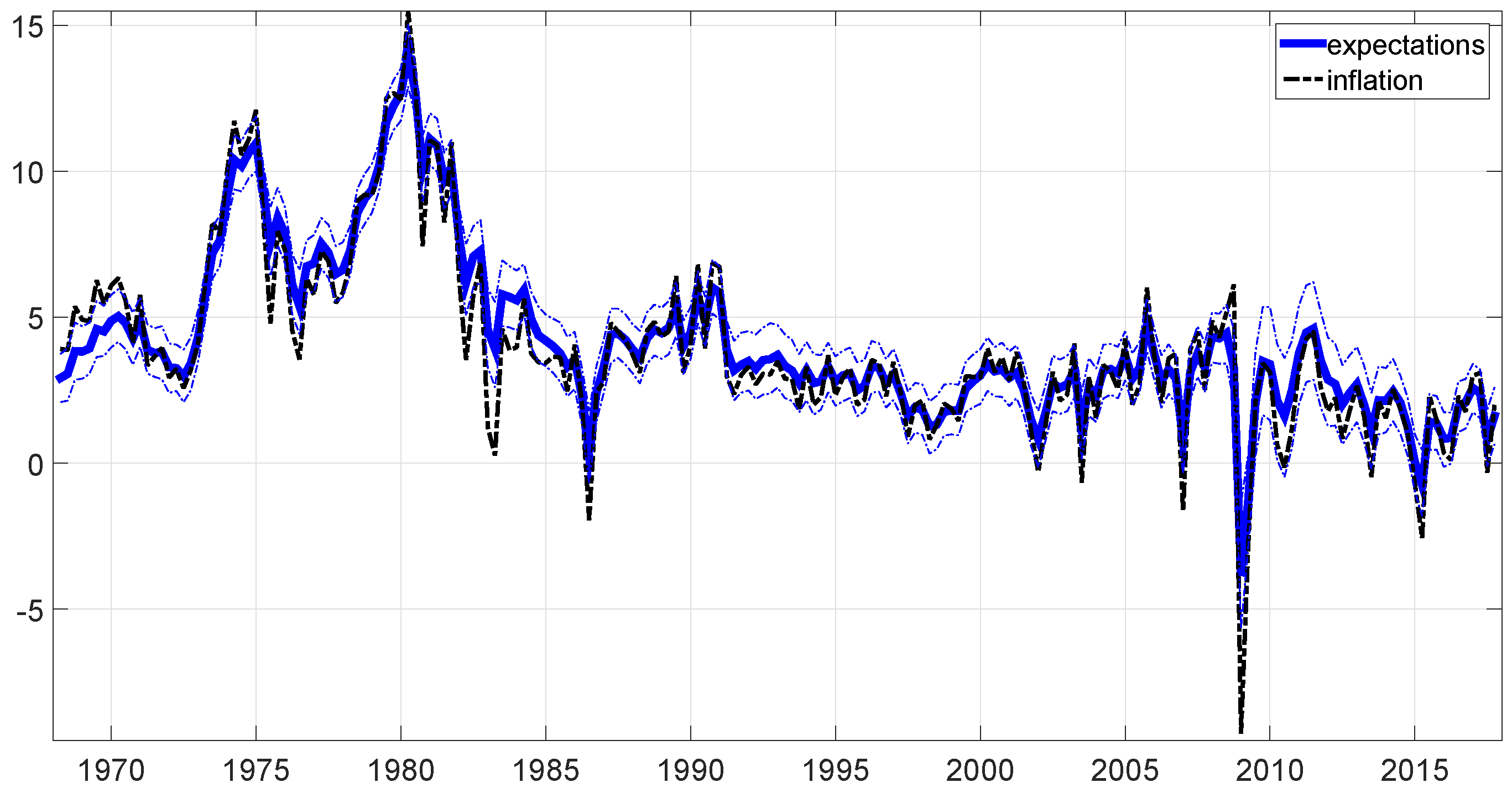
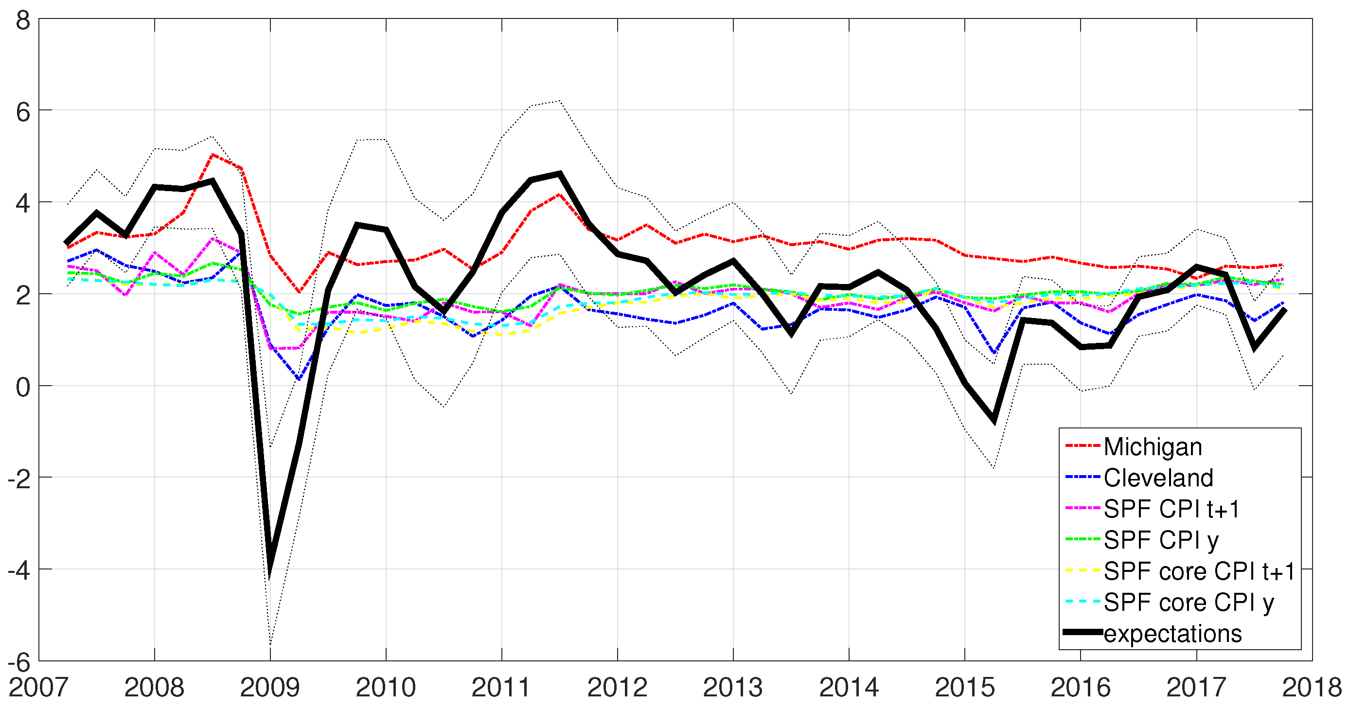
4.1. Comparison with the Observable Data on Expectations
5. Conclusions
Conflicts of Interest
Appendix A. The Markov Chain Monte Carlo Procedure
- Values of and can be sampled from these Inverse Wishart distributions.
- Values of B and can be sampled from these distributions.
- Start with some initial values for the history and the parameters
- draw a history from and a value from ;
- draw a history from and a value from ;
- draw B from and from ;
- go back to point 2.

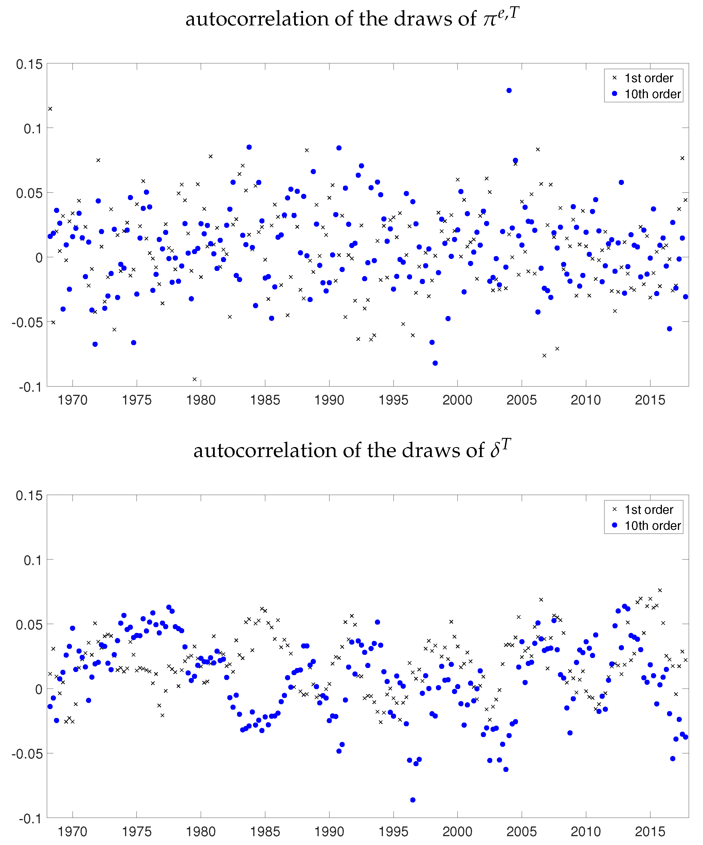
| 1st OrderAutocorrelation | 10th OrderAutocorrelation | |
|---|---|---|
| 0.0370 | 0.0409 | |
| 0.0719 | 0.0273 | |
| 0.0088 | −0.0003 | |
| 0.0283 | 0.0304 | |
| 0.0674 | 0.0034 | |
| 0.0754 | 0.0299 | |
| 0.0051 | 0.0524 |
References
- Baştürk, Nalan, Cem Çakmakli, S. Pinar Ceyhan, and Herman K. van Dijk. 2014. Posterior-Predictive Evidence On Us Inflation Using Extended New Keynesian Phillips Curve Models With Non-Filtered Data. Journal of Applied Econometrics 29: 1164–82. [Google Scholar] [CrossRef]
- Bernanke, Ben. 2010. The Economic Outlook and Monetary Policy. Speech delivered at the Federal Reserve Bank of Kansas City Economic Symposium, Jackson Hole, WY, USA, August 27. [Google Scholar]
- Binder, Carola Conces. 2015. Whose expectations augment the Phillips curve? Economics Letters 136: 35–8. [Google Scholar] [CrossRef]
- Blanchard, Olivier. 2016. The Phillips Curve: Back to the ’60s? American Economic Review 106: 31–4. [Google Scholar] [CrossRef]
- Blanchard, Olivier, Eugenio Cerutti, and Lawrence Summers. 2015. Inflation and Activity—Two Explorations and their Monetary Policy Implications. NBER Working Paper 21726, National Bureau of Economic Research, Cambridge, MA, USA. [Google Scholar]
- Carter, C. K., and R. Kohn. 1994. On Gibbs sampling for state space models. Biometrika 81: 541–53. [Google Scholar] [CrossRef]
- Chan, Joshua C. C., Todd E. Clark, and Gary Koop. 2015. A New Model of Inflation, Trend Inflation, and Long-Run Inflation Expectations. Working paper 15-20, Federal Reserve Bank of Cleveland, Cleveland, OH, USA. [Google Scholar]
- Cogley, Timothy, and Thomas J. Sargent. 2001. Evolving Post-World War II U.S. Inflation Dynamics. NBER Macroeconomics Annual 16: 331–73. [Google Scholar]
- Coibion, Olivier, and Yuriy Gorodnichenko. 2015. Is the Phillips Curve Alive and Well after All? Inflation Expectations and the Missing Disinflation. American Economic Journal: Macroeconomics 7: 197–232. [Google Scholar] [CrossRef]
- Coibion, Olivier, Yuriy Gorodnichenko, and Rupal Kamdar. 2017. The Formation of Expectations, Inflation and the Phillips Curve. NBER Working Papers 23304, National Bureau of Economic Research, Inc., Cambridge, MA, USA. [Google Scholar]
- Galì, Jordi. 2008. Monetary Policy, Inflation and the Business Cycle: An Introduction to the New Keynesian Framework. Princeton: Princeton University Press. [Google Scholar]
- Haubrich, Joseph G., George Pennacchi, and Peter H. Ritchken. 2008. Estimating Real and Nominal Term Structures Using Treasury Yields, Inflation, Inflation Forecasts, and Inflation Swap Rates. Working paper 08-10, Federal Reserve Bank of Cleveland, Cleveland, OH, USA. [Google Scholar]
- Kozicki, Sharon, and P. A. Tinsley. 2012. Effective Use of Survey Information in Estimating the Evolution of Expected Inflation. Journal of Money, Credit and Banking 44: 145–69. [Google Scholar] [CrossRef]
- Lopez-Perez, Víctor. 2017. Do professional forecasters behave as if they believed in the New Keynesian Phillips Curve for the euro area? Empirica 44: 147–74. [Google Scholar] [CrossRef]
- McCallum, Bennett T. 1976. Rational Expectations and the Estimation of Econometric Models: An Alternative Procedure. International Economic Review 17: 484–90. [Google Scholar] [CrossRef]
- Mertens, Elmar. 2016. Measuring the Level and Uncertainty of Trend Inflation. The Review of Economics and Statistics 98: 950–67. [Google Scholar] [CrossRef]
- Mertens, Elmar, and James M. Nason. 2017. Inflation and Professional Forecast Dynamics: An Evaluation of Stickiness, Persistence, and Volatility. CAMA Working Papers 2017-60, Centre for Applied Macroeconomic Analysis, Crawford School of Public Policy, The Australian National University, Canberra, Australia. [Google Scholar]
- Nason, James M., and Gregor W. Smith. 2013. Reverse Kalman Filtering U.S. Inflation with Sticky Professional Forecasts. Working Papers 13-34, Federal Reserve Bank of Philadelphia, Philadelphia, PA, USA. [Google Scholar]
- Nunes, Ricardo. 2010. Inflation Dynamics: The Role of Expectations. Journal of Money, Credit and Banking 42: 1161–72. [Google Scholar] [CrossRef]
- Primiceri, Giorgio E. 2005. Time Varying Structural Vector Autoregressions and Monetary Policy. The Review of Economic Studies 72: 821–52. [Google Scholar] [CrossRef]
- Primiceri, Giorgio E. 2006. Why Inflation Rose and Fell: Policy-Makers’ Beliefs and U. S. Postwar Stabilization Policy. The Quarterly Journal of Economics 121: 867–901. [Google Scholar] [CrossRef]
- Roberts, John. 1995. New Keynesian Economics and the Phillips Curve. Journal of Money, Credit and Banking 27: 975–84. [Google Scholar] [CrossRef]
- Staiger, Douglas, James H. Stock, and Mark W. Watson. 2001. Prices, Wages and the U.S. NAIRU in the 1990s. Working Paper 8320, National Bureau of Economic Research, Cambridge, MA, USA. [Google Scholar]
- Stock, James H., and Mark W. Watson. 2007. Why Has U.S. Inflation Become Harder to Forecast? Journal of Money, Credit and Banking 39: 3–33. [Google Scholar] [CrossRef]
- Stock, James H., and Mark W. Watson. 2016. Core Inflation and Trend Inflation. The Review of Economics and Statistics 98: 770–84. [Google Scholar] [CrossRef]
- Svensson, Lars E. O. 2015. The Possible Unemployment Cost of Average Inflation below a Credible Target. American Economic Journal: Macroeconomics 7: 258–96. [Google Scholar] [CrossRef]
| 1 | See Coibion and Gorodnichenko (2015) for a discussion of the interpretation of this variable in alternative structural models of the Phillips Curve. |
| 2 | The random walk process assumed in (3) is quite general, but other approaches to model long run inflation expectations within the context of the NKPC are also possible. For instance, see the framework used in Baştürk et al. (2014). |
| 3 | The natural rate of unemployment could also be estimated using a similar econometric model as the one employed for . However, treating both the natural rate and inflation expectations as unknown would have made the estimation of the full framework quite challenging. Given that the focus of this paper is on expectations, I decided to simply use the measure of the natural rate computed by the CBO and treat the variable as fully observable. |
| 4 | Monthly variables were transformed into quarterly by taking averages of the months in the quarter. The data for and were all downloaded from the FRED Federal Reserve Bank of St. Louis webpage. |
| 5 | Two additional exercises use the median forecast of price changes over the next 12 months for different demographic groups, and the median forecast of price changes over the next 5 to 10 years. As for the baseline series, these additional data were obtained from the University of Michigan Surveys of Consumers webpage and transformed into quarterly observations. |
| 6 | The methodology used to compute this series is described in Haubrich et al. (2008). |
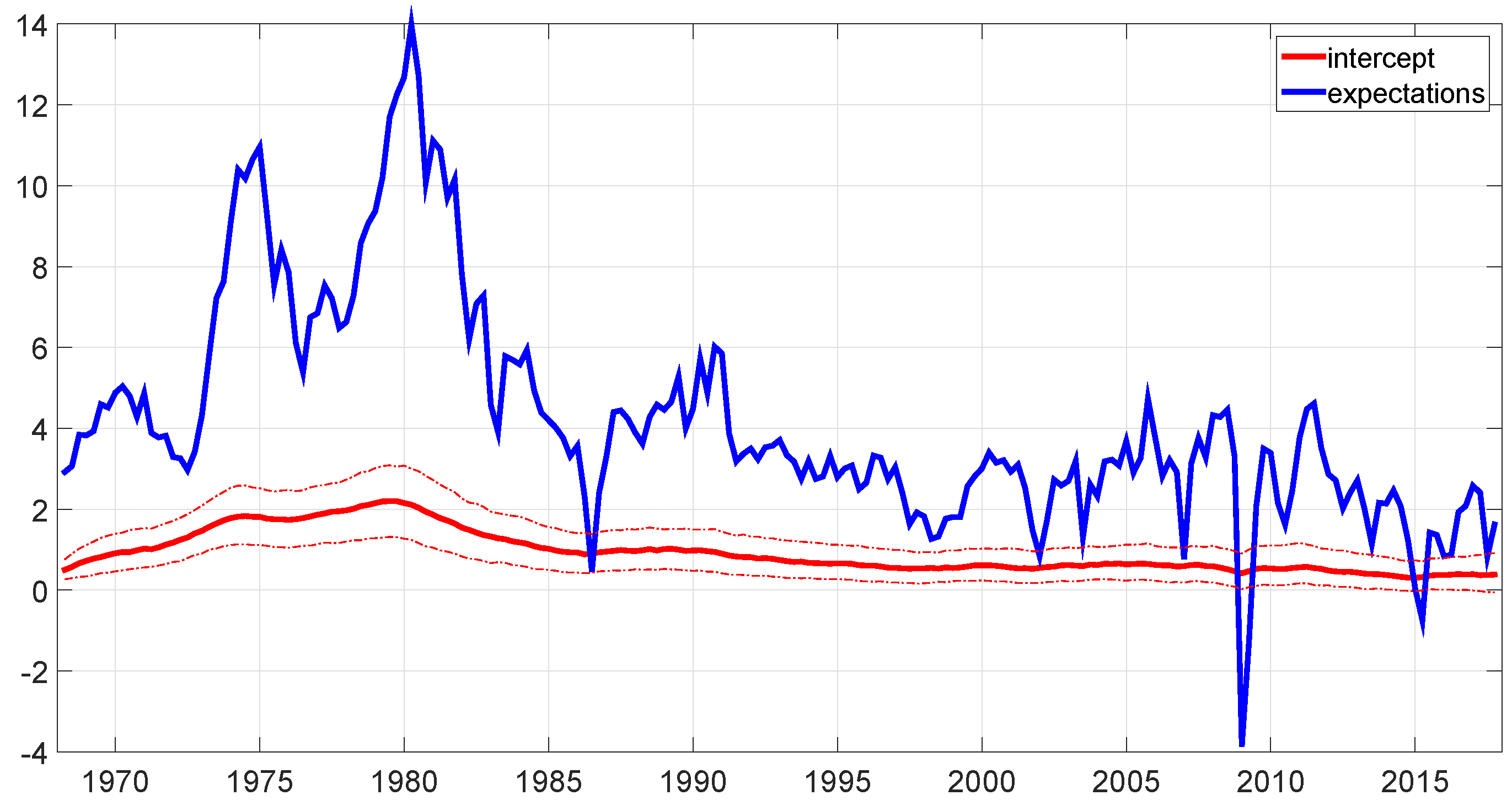
| 7 | Equation (4) is not exactly the same as the one estimated by Coibion and Gorodnichenko (2015), because I do not include the indicator variable by itself as an additional variable. Thus, the model described by (4) is only able to capture a shift in the slope , but not in the intercept . This choice was forced by the fact that adding one more parameter considerably decreased the precision of all the estimated parameters of the NKPC. Thus, I decided to include the indicator variable only in the form of an interaction with which still allows the model to incorporate possible shifts in the slope of the NKPC, without increasing the dispersion of the estimates to a troublesome degree. |
| 8 | Notice that these are univariate Inverse Whisart distributions, which are equivalent to Inverse Gamma distributions. |
| 9 | I experimented with a range of different values for and for the mean in the prior for . I also tried to increase the dispersion of the Normal priors (8), (9), and (10), by multiplying the original variances by 4. Finally, I included factors and in (11) and (12) in addition to (13), and I experimented with different values for these factors. Neither the results nor the convergence of the algorithm were substantially affected by any of these changes. |
| 10 | The estimated value of is not statistically significant in Coibion and Gorodnichenko (2015) as well. |
| 11 | |
| 12 | For several of the inflation forecasts measures, the data are only available for some of these sub-periods. In each case, I only computed the statistics of interest if I had data for all the quarters in the sub-period. |
| 13 | |
| 14 | For more details, see Carter and Kohn (1994). |


| 16th | Median | 84th | |
|---|---|---|---|
| −0.3075 | −0.0597 | 0.1461 | |
| −0.6963 | −0.4990 | −0.3246 | |
| −0.1570 | 0.2976 | 0.7105 | |
| 0.6881 | 0.7606 | 0.8508 | |
| 0.9464 | 1.2597 | 1.7059 | |
| 1.0767 | 1.9009 | 2.6421 | |
| 0.0113 | 0.0273 | 0.0554 |
| Correlations | Sample | 16th | Median | 84th |
|---|---|---|---|---|
| Michigan | 1978–2017 | 0.8414 | 0.8620 | 0.8830 |
| Cleveland | 1982–2017 | 0.5092 | 0.6459 | 0.7250 |
| SPF CPI (t) | 1981–2017 | 0.6967 | 0.7777 | 0.8185 |
| SPF CPI () | 1981–2017 | 0.5990 | 0.7065 | 0.7699 |
| SPF CPI (y) | 1981–2017 | 0.5564 | 0.6603 | 0.7359 |
| SPF core CPI (t) | 2007–2017 | −0.0625 | 0.1810 | 0.4196 |
| SPF core CPI () | 2007–2017 | −0.2842 | 0.0055 | 0.3203 |
| SPF core CPI (y) | 2007–2017 | −0.2712 | 0.0221 | 0.3395 |
| Correlations | Sample | 16th | Median | 84th | Sample | 16th | Median | 84th |
|---|---|---|---|---|---|---|---|---|
| Michigan | 1978–2006 | 0.8983 | 0.9128 | 0.9265 | 2007–2017 | 0.3823 | 0.4650 | 0.5370 |
| Cleveland | 1982–2006 | 0.5690 | 0.6415 | 0.7071 | 2007–2017 | 0.4175 | 0.6085 | 0.7325 |
| SPF CPI (t) | 1981–2006 | 0.7206 | 0.7630 | 0.7940 | 2007–2017 | 0.5877 | 0.7251 | 0.8095 |
| SPF CPI () | 1981–2006 | 0.6933 | 0.7442 | 0.7916 | 2007–2017 | 0.2634 | 0.4956 | 0.6755 |
| SPF CPI (y) | 1981–2006 | 0.6574 | 0.7145 | 0.7763 | 2007–2017 | 0.0586 | 0.3286 | 0.5771 |
| SPF core CPI (t) | - | - | - | - | 2007–2017 | −0.0625 | 0.1810 | 0.4196 |
| SPF core CPI () | - | - | - | - | 2007–2017 | −0.2842 | 0.0055 | 0.3203 |
| SPF core CPI (y) | - | - | - | - | 2007–2017 | −0.2712 | 0.0221 | 0.3395 |
| Average | Variance | Autocorrelation | |
|---|---|---|---|
| Sample period 1978–2017 | |||
| Estimated | 3.7903 | 7.4360 | 0.9188 |
| Michigan | 3.6138 | 2.8630 | 0.9554 |
| Sample period 1982–2017 | |||
| Estimated | 3.0425 | 2.3068 | 0.7468 |
| Cleveland | 2.9029 | 1.4444 | 0.9385 |
| Sample period 1981–2017 | |||
| Estimated | 3.1243 | 2.7763 | 0.7733 |
| SPF CPI (t) | 2.8799 | 2.6685 | 0.6252 |
| SPF CPI () | 2.9583 | 1.5487 | 0.9393 |
| SPF CPI (y) | 3.0597 | 1.5025 | 0.9788 |
| Sample period 2007–2017 | |||
| Estimated | 2.1912 | 2.6422 | 0.5640 |
| SPF core CPI (t) | 1.8103 | 0.1723 | 0.6025 |
| SPF core CPI () | 1.8383 | 0.1327 | 0.8820 |
| SPF core CPI (y) | 1.9094 | 0.0946 | 0.8898 |
| Average | 1978–1984 | 1985–2006 | 2007–2017 |
|---|---|---|---|
| Estimated | 8.3280 | 3.1279 | 2.1912 |
| Michigan | 6.2940 | 3.0295 | 3.0643 |
| Cleveland | - | 3.1651 | 1.7018 |
| SPF CPI (t) | - | 3.0346 | 1.8138 |
| SPF CPI () | - | 3.0678 | 1.9542 |
| SPF CPI (y) | - | 3.1531 | 2.0488 |
| SPF core CPI (t) | - | - | 1.8103 |
| SPF core CPI () | - | - | 1.8383 |
| SPF core CPI (y) | - | - | 1.9094 |
| Variance | 1978–1984 | 1985–2006 | 2007–2017 |
|---|---|---|---|
| Estimated | 8.8005 | 1.1633 | 2.6422 |
| Michigan | 6.3941 | 0.2493 | 0.3301 |
| Cleveland | - | 0.5958 | 0.3048 |
| SPF CPI (t) | - | 1.2955 | 2.0618 |
| SPF CPI () | - | 0.7813 | 0.2251 |
| SPF CPI (y) | - | 0.7306 | 0.0670 |
| SPF core CPI (t) | - | - | 0.1723 |
| SPF core CPI () | - | - | 0.1327 |
| SPF core CPI (y) | - | - | 0.0946 |
| Autocorrelation | 1978–1984 | 1985–2006 | 2007–2017 |
|---|---|---|---|
| Estimated | 0.9136 | 0.7582 | 0.5640 |
| Michigan | 0.9495 | 0.7061 | 0.6431 |
| Cleveland | - | 0.9179 | 0.5220 |
| SPF CPI (t) | - | 0.5604 | 0.3198 |
| SPF CPI () | - | 0.9129 | 0.5019 |
| SPF CPI (y) | - | 0.9677 | 0.7446 |
| SPF core CPI (t) | - | - | 0.6025 |
| SPF core CPI () | - | - | 0.8820 |
| SPF core CPI (y) | - | - | 0.8898 |
| 1990–2006 | 2007–2017 | 1990–2017 | |
|---|---|---|---|
| Correlation with | |||
| Michigan | 0.5851 | 0.4650 | 0.4722 |
| [16th, 84th] | [0.4931, 0.6574] | [0.3823, 0.5370] | [0.3904, 0.5253] |
| Michigan 5 years | 0.4695 | 0.3608 | 0.4091 |
| [16th, 84th] | [0.3489, 0.5816] | [0.2374, 0.4499] | [0.3422, 0.4800] |
| Variance | |||
| Estimated | 0.9228 | 2.6422 | 1.6963 |
| Michigan | 0.2204 | 0.3301 | 0.2648 |
| Michigan 5 years | 0.2294 | 0.0322 | 0.1842 |
| Autocorrelation | |||
| Estimated | 0.7279 | 0.5640 | 0.6347 |
| Michigan | 0.6597 | 0.6431 | 0.6579 |
| Michigan 5 years | 0.9672 | 0.7844 | 0.9602 |
| Correlations | 16th | Median | 84th |
|---|---|---|---|
| 0.8414 | 0.8620 | 0.8830 | |
| Age groups (sample 1978–2017) | |||
| 18–34 | 0.8442 | 0.8658 | 0.8906 |
| 35–54 | 0.8528 | 0.8731 | 0.8938 |
| 55+ | 0.7654 | 0.7932 | 0.8152 |
| Regions (sample 1978–2017) | |||
| West | 0.8382 | 0.8593 | 0.8831 |
| North Central | 0.8263 | 0.8482 | 0.8685 |
| Northeast | 0.8522 | 0.8727 | 0.8912 |
| South | 0.8282 | 0.8499 | 0.8713 |
| Gender (sample 1978–2017) | |||
| Male | 0.8493 | 0.8693 | 0.8883 |
| Female | 0.8290 | 0.8514 | 0.8732 |
| Income group (sample 1979–2017) | |||
| Bottom 33% | 0.7315 | 0.7617 | 0.7853 |
| Middle 33% | 0.7913 | 0.8160 | 0.8401 |
| Top 33% | 0.8189 | 0.8452 | 0.8675 |
| Education level (sample 1978–2017) | |||
| High School or less | 0.7908 | 0.8175 | 0.8383 |
| Some college | 0.8186 | 0.8410 | 0.8614 |
| College degree | 0.8576 | 0.8790 | 0.9014 |
© 2018 by the author. Licensee MDPI, Basel, Switzerland. This article is an open access article distributed under the terms and conditions of the Creative Commons Attribution (CC BY) license (http://creativecommons.org/licenses/by/4.0/).
Share and Cite
Rondina, F. Estimating Unobservable Inflation Expectations in the New Keynesian Phillips Curve. Econometrics 2018, 6, 6. https://doi.org/10.3390/econometrics6010006
Rondina F. Estimating Unobservable Inflation Expectations in the New Keynesian Phillips Curve. Econometrics. 2018; 6(1):6. https://doi.org/10.3390/econometrics6010006
Chicago/Turabian StyleRondina, Francesca. 2018. "Estimating Unobservable Inflation Expectations in the New Keynesian Phillips Curve" Econometrics 6, no. 1: 6. https://doi.org/10.3390/econometrics6010006
APA StyleRondina, F. (2018). Estimating Unobservable Inflation Expectations in the New Keynesian Phillips Curve. Econometrics, 6(1), 6. https://doi.org/10.3390/econometrics6010006