Do Seasonal Adjustments Induce Noncausal Dynamics in Inflation Rates?

Abstract

This paper investigates the effect of seasonal adjustment filters on the identification of mixed causal-noncausal autoregressive models. By means of Monte Carlo simulations, we find that standard seasonal filters induce spurious autoregressive dynamics on white noise series, a phenomenon already documented in the literature. Using a symmetric argument, we show that those filters also generate a spurious noncausal component in the seasonally adjusted series, but preserve (although amplify) the existence of causal and noncausal relationships. This result has has important implications for modelling economic time series driven by expectation relationships. We consider inflation data on the G7 countries to illustrate these results.

1. Introduction

Most empirical macroeconomic studies are based on seasonally adjusted data. Various methods have been proposed in the literature aiming at removing unobserved seasonal patterns without affecting other properties of the time series. Just as the misspecification of a trend may cause spurious cycles in detrended data (e.g., Nelson and Kang 1981), a wrongly specified pattern at the seasonal frequency might have very undesirable effects (see, e.g., Ghysels and Perron 1993; Maravall 1993). A substantial literature focuses on the effects of seasonal adjustment for testing on unit roots, structural change and bias using various autoregressive processes: Ghysels (1990), Ghysels and Perron (1993) and Del Barrio Castro and Osborn (2004) consider the conventional AR, ARMA and periodic AR processes respectively. To the best of our knowledge, there is no result on the consequences of seasonal adjustment for mixed causal-noncausal autoregressive (MAR) process. As discussed in Hecq et al. (2016), MAR models are able to generate features that previously could only be obtained using highly nonlinear and complex models. This includes the possibility of periodic and speculative bubble processes. Following Gouriéroux et al. (2016) and Lanne and Saikkonen (2011), MAR models can also constitute stationary solutions for rational expectation models.

The present paper examines the effect of the linear approximation of X-11 seasonal adjustment on the selection of mixed causal-noncausal autoregressive processes. We focus on whether (non)causality in the seasonally adjusted time series is preserved. It is shown that the linear X-11 seasonal adjustment affects the autocovariance function of different MAR specifications of the same autoregressive order in exactly the same way. This is due to the well-known fact that the autocovariance functions and thus spectral densities of these processes are the same (up to a rescaled variance). Since the maximum likelihood procedure used to estimate MAR models exploits more information than solely second-order properties of the process, backward- and forward-looking dynamics are to a great extent preserved in the time series. A simulation study confirms this hypothesis and additionally shows that X-11 seasonal adjustment of white noise series introduces spurious dynamics, which are purely causal or purely noncausal with equal frequency. We investigate the effect of seasonal adjustment on selecting MAR models for inflation rates of the G7 countries Canada, France, Germany, Italy, Japan, the United Kingdom and the United States. It has been found that the distinctive features of inflation can be captured well by MAR models due to their closeness to rational expectation models (Lanne and Luoto 2012, 2013; Lanne et al. 2012a). Another reason why noncausal models can provide a good fit to this type of data is the property that they, at least in the Cauchy case, exhibit a causal recursive double autoregressive structure (Gouriéroux and Zakoïan 2016). This means that one can account for ARCH-type effects in a series by including a noncausal component in the model equation for the conditional mean. For this reason, it is of interest to see how sensitive model selection of inflation is with respect to seasonal adjustment methods.

The remainder of this paper is organized as follows. Section 2 formalizes the notion of mixed causal-noncausal models and comments on the identifiability and estimation of such models. Section 3 discusses seasonal adjustment methods based on simple linear filters and mentions their merits and potential pitfalls. The results of the simulation study are collected in Section 4. Section 5 considers both raw and seasonally adjusted quarterly inflation rates for the G7 countries and shows the effects of seasonal adjustment on the selection of MAR($r,s$) models. Section 6 summarizes and concludes.

2. Mixed Causal-Noncausal Models

Brockwell and Davis (1991) originally advocated the use of noncausal models as they offer the possibility to rewrite a process with explosive roots in calendar time into a process in reverse time with roots outside the unit circle. Additional important empirical features of the noncausal approach have been put forward in the recent literature. Beyond the improvement in terms of forecasting accuracy (see e.g., Lanne et al. 2012b) as well as their closeness to the concept of nonfundamental shocks (see e.g., Alessi et al. 2011), simple linear noncausal models are able to mimic nonlinear processes such as bubbles or asymmetric cycles (see e.g., Gouriéroux and Zakoïan 2016; Hecq et al. 2016; Fries and Zakoïan 2017).

2.1. Model Representation

The univariate mixed causal-noncausal autoregressive model MAR($r,s$) for a stationary time series $y_t,(t=1,\dots ,T)$ is written as

$$\begin{array}{ccc}\hfill (1-{\varphi }_{1}L-...-{\varphi }_r{L}^r)(1-{\phi }_1{L}^{-1}-...-{\phi }_s{L}^{-s})y_t& =& {\epsilon }_t,\hfill \end{array}$$

(1)

$$\begin{array}{ccc}\hfill \varphi \left(L\right)\phi \left(L^{-1}\right)y_t& =& {\epsilon }_t,\hfill \end{array}$$

(2)

with L being the backshift operator, i.e., $L{y}_t=y_{t-1}$ gives lags and $L^{-1}{y}_t=y_{t+1}$ produces leads. The error term ${\epsilon }_t$ is $iid$ non-Gaussian. When ${\phi }_1=\dots ={\phi }_s=0,$ the process $y_t$ is a purely causal autoregressive process, denoted AR(r,0) or simply AR($r)$:

$$\varphi \left(L\right)y_t={\epsilon }_t.$$

(3)

Model specification (3) can be seen as the standard backward-looking AR process, with $y_t$ being regressed on $y_{t-1}$ up to $y_{t-r}$. The process in (2) becomes a purely noncausal AR($0,s)$ model

$$\phi \left(L^{-1}\right)y_t={\epsilon }_t,$$

(4)

when ${\varphi }_1=\dots ={\varphi }_r=0.$ Model specification (4) is the counterpart of (3), since it is a purely forward-looking AR process. That is, $y_t$ does not depend on its past values, but rather on its future values $y_{t+1}$ up to $y_{t+s}$. Models of the form (2) that contain both lags and leads of the dependent variable are called mixed causal-noncausal models. In the sequel of this paper, $\varphi \left(L\right)$ and $\phi \left(L^{-1}\right)$ denote the causal and noncausal polynomials, while boldfaced $\mathit{\varphi }={[{\varphi }_1,\dots ,{\varphi }_r]}^{\prime }$ and $\mathit{\phi }={[{\phi }_1,\dots ,{\phi }_s]}^{\prime }$ represent the corresponding parameter vectors.

The roots of both the causal and noncausal polynomials are assumed to lie outside the unit circle, that is $\varphi \left(z\right)=0$ and $\phi \left(z\right)=0$ for $\left|z\right|>1$ respectively. These conditions imply that the series $y_t$ admits a two-sided moving average (MA) representation $y_t={\sum }_{j=-\infty }^{\infty }{\psi }_j{\epsilon }_{t-j},$ such that ${\psi }_j=0$ for all $j<0$ implies a purely causal process $y_t$ (w.r.t. ${\epsilon }_t$) and a purely noncausal model when ${\psi }_j=0$ for all $j>0$.

2.2. Estimation

The non-Gaussianity assumption ensures the identifiability of the causal and the noncausal part (Breidt et al. 1991). In this paper, we consider a non-standardized t-distribution for the error process. Lanne and Saikkonen (2011) show that the parameters of mixed causal-noncausal autoregressive models of the form (2) can be consistently estimated by approximate maximum likelihood (AML).1 Let $({\epsilon }_1,\dots ,{\epsilon }_T)$ be a sequence of $iid$ zero mean t-distributed random variables, then its joint probability density function can be characterized as

$$f_{\epsilon }({\epsilon }_1,\dots ,{\epsilon }_T|\sigma ,\nu )=\prod _{t=1}^T\frac{\mathrm{\Gamma }\left(\frac{\nu +1}{2}\right)}{\mathrm{\Gamma }\left(\frac{\nu }{2}\right)\sqrt{\pi \nu }\sigma }{\left(1+\frac{1}{\nu }{\left(\frac{{\epsilon }_t}{\sigma }\right)}^2\right)}^{-\frac{\nu +1}{2}}.$$

The corresponding (approximate) log-likelihood function, conditional on the observed data $y=(y_1,\dots ,y_T)$ can be formulated as

$$\begin{array}{cc}\hfill l_y(\mathit{\varphi },\mathit{\phi },\mathit{\lambda },\alpha |y)& =\left(T-p\right)\left[ln\left(\mathrm{\Gamma }((\nu +1)/2)\right)-ln\left(\sqrt{\nu \pi }\right)-ln\left(\mathrm{\Gamma }(\nu /2)\right)-ln\left(\sigma \right)\right]\\ & -(\nu +1)/2{\sum }_{t=r+1}^{T-s}ln(1+{((\varphi \left(L\right)\phi \left(L^{-1}\right)y_t-\alpha )/\sigma )}^2/\nu ),\end{array}$$

(5)

where $p=r+s$. The distributional parameters are collected in $\mathit{\lambda }={[\sigma ,\nu ]}^{\prime }$, with $\sigma$ representing the scale parameter and $\nu$ the degrees of freedom. $\alpha$ denotes an intercept that could be introduced in model (2), $\mathrm{\Gamma }(·)$ denotes the gamma function. Thus, the AML estimator corresponds to the solution

$${\widehat{\mathit{\theta }}}_{ML}=arg\underset{\mathit{\theta }\in \mathsf{\Theta }}{max}{l}_y\left(\mathit{\theta }\right|y),$$

with $\mathit{\theta }={[{\mathit{\varphi }}^{\prime },{\mathit{\phi }}^{\prime },{\mathit{\lambda }}^{\prime },\alpha ]}^{\prime }$ and $\mathsf{\Theta }$ is a permissible parameter space containing the true value of $\mathit{\theta }$, say ${\mathit{\theta }}_0$, as an interior point. Since an analytical solution of the score function is not directly available, gradient based (numerical) procedures (e.g., BHHH and BFGS) can be used to find ${\widehat{\mathit{\theta }}}_{ML}$. If $\nu >2$, and hence $\mathbb{E}\left(\right|{\epsilon }_t{|}^2)<\infty$, the AML estimator is $\sqrt{T}$-consistent and asymptotically normal. Lanne and Saikkonen (2011) also show that a consistent estimator of the limiting covariance matrix is obtained from the standardized Hessian of the log-likelihood. For the estimation and selection of mixed causal-noncausal models we follow the procedure proposed in Hecq et al. (2016). Namely, we first estimate by OLS conventional autoregessive models and identify the autoregressive order p that deletes all serial correlation from the residuals. Once this order p has been established, we estimate all combinations of MAR($r,s$) models for which $r+s=p$. The model with the highest log-likelihood in (5) at the estimated parameters is selected as final model. It has to be noted that this procedure is not free from misspecification of the noncausal order s for a fixed p as shown in Gouriéroux and Jasiak (2017).

3. Seasonal Adjustment Methods

Seasonal adjustment of data series has received a lot of attention in the econometric and statistical literature; an extensive overview can be found in Bell and Hillmer (2002). The insight that seasonality might alter the legibility of the trend and the cyclical component led to the development of moving averages that adjust series at their seasonal frequencies. These moving averages are computed using centered, symmetric linear filters of the form

$${\mathsf{\Psi }}^{SA}(L,L^{-1})=c_0+\sum _{j=1}^k{c}_j(L^j+L^{-j}).$$

(6)

As these filters are frequently present in seasonal adjustment methods used at statistical agencies (see e.g., Ghysels and Perron 1993), we focus on them in the simulation study of this paper.

3.1. The Linear X-11 Seasonal Filter

In particular, we focus on the linear approximation of quarterly X-11 seasonal adjustment, ${\mathsf{\Psi }}_{X-11}^{SA}(L,L^{-1})$, which is a moving average of order 57 with weights that sum up to one. The filter has both leads and lags, as it takes 28 quarters before and 28 quarters after every data point into account. This linear approximation represents the result of applying a sequence of symmetric two-sided moving average filters designed to decompose the series into mutually orthogonal trend, seasonal and irregular components (Del Barrio Castro and Osborn 2004). These operations results in subtracting the estimated seasonal component from the observed series, which gives the linear X-11 seasonal adjustment its representation as time-invariant filtering operation.

Table 1. Filter weights of the linear quarterly X-11 filter.

Lags/Leads		Lags/Leads		Lags/Leads
0	0.856	10	0.025	20	$-0.003$
1	0.051	11	0.012	21	<0.001
2	0.041	12	$-0.053$	22	0.002
3	0.050	13	0.021	23	<0.001
4	$-0.140$	14	0.016	24	<0.001
5	0.055	15	$-0.005$	25	<0.001
6	0.034	16	$-0.010$	26	<0.001
7	0.029	17	<0.001	27	<0.001
8	$-0.097$	18	0.008	28	<0.001
9	0.038	19	$-0.002$

shows the final weights, rounded to 3 decimals for expository purposes (see e.g., Ghysels and Perron 1993).

The Census X-11 program was the most widely applied adjustment procedure by statistical agencies. More recent versions, such as the so-called X-13-ARIMA, consist of first identifying and estimating an ARMA model on the series (with outliers, breaks, calendar effects, etc.) with the aim to extrapolate the variable in the past and in the future before taking a set of moving average filters similar to (6). This is done to preserve the number of observations that would be lost in the X-11 method without applying back- and forecasting operations. Many famous statistical agencies and database providers like OECD, NBER and BEA use these methods in order to seasonally adjust most of their series. Additionally, in most econometric software programs (e.g., EViews, RATS, SAS and gretl) various seasonal adjustment approaches based on the X-11 filter are either directly implemented or available through add-on packages that provide these methods. We consider simple linear filters in this study because we want to isolate the effects coming from the moving average adjustment.

3.2. Properties of Seasonal Adjustment

The desired property for any seasonal adjustment method is that it only affects the time series of interest at the seasonal frequencies (Ghysels et al. 1993). This requirement is not always fulfilled. For example, suppose we have a zero-mean data series $y_t$ which is seasonally adjusted by a linear filter like in (6), with $k=1$ (for the sake of simplicity). Then the seasonally adjusted series $y_t^{SA}$ has first-order autocovariance equal to:

$$\begin{array}{cc}\hfill \mathrm{Cov}(y_t^{SA},y_{t-1}^{SA})& =\mathrm{Cov}\left(({\psi }_1{y}_{t-1}+{\psi }_0{y}_t+{\psi }_{-1}{y}_{t+1}),({\psi }_1{y}_{t-2}+{\psi }_0{y}_{t-1}+{\psi }_{-1}{y}_t)\right)\hfill \\ & ={\psi }_1{\psi }_0\mathbb{E}\left(y_{t-1}^2\right)+{\psi }_0{\psi }_{-1}\mathbb{E}\left(y_t^2\right)\hfill \\ & =2{\psi }_0{\psi }_1{\sigma }^2,\hfill \end{array}$$

since ${\psi }_i={\psi }_{-i}$ for all i in the X-11 filter. That is, the seasonally adjusted series $y_t^{SA}$ now has existing autovariances between observations at t and $t-h$ for $h\ne 0$. Since the autocovariance function is fully symmetric, these autocovariances also exist between observations t and $t+h$ for $h\ne 0$. From convolution theory, it is well-known that the autocorrelation of the linear filter is convolved with the autocorrelation of the series. In other words, the autocorrelation of ${\mathsf{\Psi }}_{X-11}^{SA}(L,L^{-1})$ acts as a smoothing filter on the autocorrelation of $y_t$. However, if $y_t$ is a white noise (or $iid$) series, these newly existing autocovariances are not due to existing dynamics in the series, but rather spuriously introduced by the seasonal adjustment filter. The special case of applying the X-11 filter to white noise has been well documented in Kaiser and Maravall (2001). We do, however, not rule out this case in our simulation study, as our main interest is to see whether seasonal adjustment filters can create spurious causal and noncausal dynamics in different data generating processes.

3.3. Seasonal Adjustment for Mixed Processes

It is common in the seasonality literature to compare the autocovariance function of processes before and after the filtering procedure. In the case of mixed causal-noncausal autoregressions, this procedure does not offer much information. Suppose $y_t$ follows an MAR($r,s$) process as in (2) with corresponding autocovariance function ${\gamma }_y(·)$ and spectrum $f_y\left(\omega \right)$. Applying the Filter Theorem, the autocovariances of the X-11 filtered process $y_t^{SA}={\mathsf{\Psi }}_{X-11}^{SA}(L,L^{-1})y_t$ can be represented as

$${\gamma }_{y^{SA}}\left(k\right)=\sum _{j=-l}^l{\gamma }_{{\mathsf{\Psi }}^{SA}}\left(j\right){\gamma }_y(k-j),$$

(7)

with $k\in \mathbb{Z}$ and $l=28$ for the X-11 filter. The sequence $\{{\gamma }_{{\mathsf{\Psi }}^{SA}}\left(j\right)$|$j\in \mathbb{Z}\}$ is given by

$${\gamma }_{{\mathsf{\Psi }}^{SA}}\left(j\right)=\sum _{i=-\infty }^{\infty }{\psi }_i{\psi }_{i+j},$$

(8)

with ${\psi }_i$ being the ith coefficient in the X-11 filter (where ${\psi }_i=0$ for $\left|i\right|>28$). However, as it is well-known that a zero-mean MAR($r,s$) process can be represented as a purely causal AR(p) with exactly the autocovariance function ${\gamma }_y(·)$ (up to rescaled variance), this measure cannot be used to distinguish between all MAR($r,s$) processes with $r+s=p$. Similarly, due to the fact that also the spectrum $f_y\left(\omega \right)$ is the same for all processes of the same total order p, the transfer function ${\mathsf{\Phi }}^{SA}\left(e^{i\omega }\right)$ and the power transfer function $|{\mathsf{\Phi }}^{SA}\left(e^{i\omega }\right){|}^2$ have exactly the same effect on the second-order properties of e.g., a MAR(2,0), MAR(1,1) and MAR(0,2) process when $p=2$. Hence, the remaining question is whether (non)causality of the process is preserved in a model selection procedure. To that end, it is interesting to investigate whether the non-Gaussian likelihood procedure can distinguish between different MAR($r,s$) specifications after X-11 seasonal adjustment.

4. Simulation Study

In this simulation study, we investigate the effect of X-11 seasonal adjustment on the model selection of various causal, noncausal and mixed causal-noncausal processes.

4.1. Purely Causal and Noncausal Processes

We consider three data generating processes for the stationary time series $y_t,y_t^{-}$ and $y_t^{+}$:

$$\begin{array}{cc}\hfill y_t^{}& =\sum _{s=1}^4{\delta }_s{D}_{s,t}+{\epsilon }_t,\hfill \\ \hfill y_t^{-}& ={\varphi }_1{y}_{t-1}^{-}+\sum _{s=1}^4{\delta }_s{D}_{s,t}+{\epsilon }_t,\hfill \\ \hfill y_t^{+}& ={\phi }_1{y}_{t+1}^{+}+\sum _{s=1}^4{\delta }_s{D}_{s,t}+{\epsilon }_t,\hfill \end{array}$$

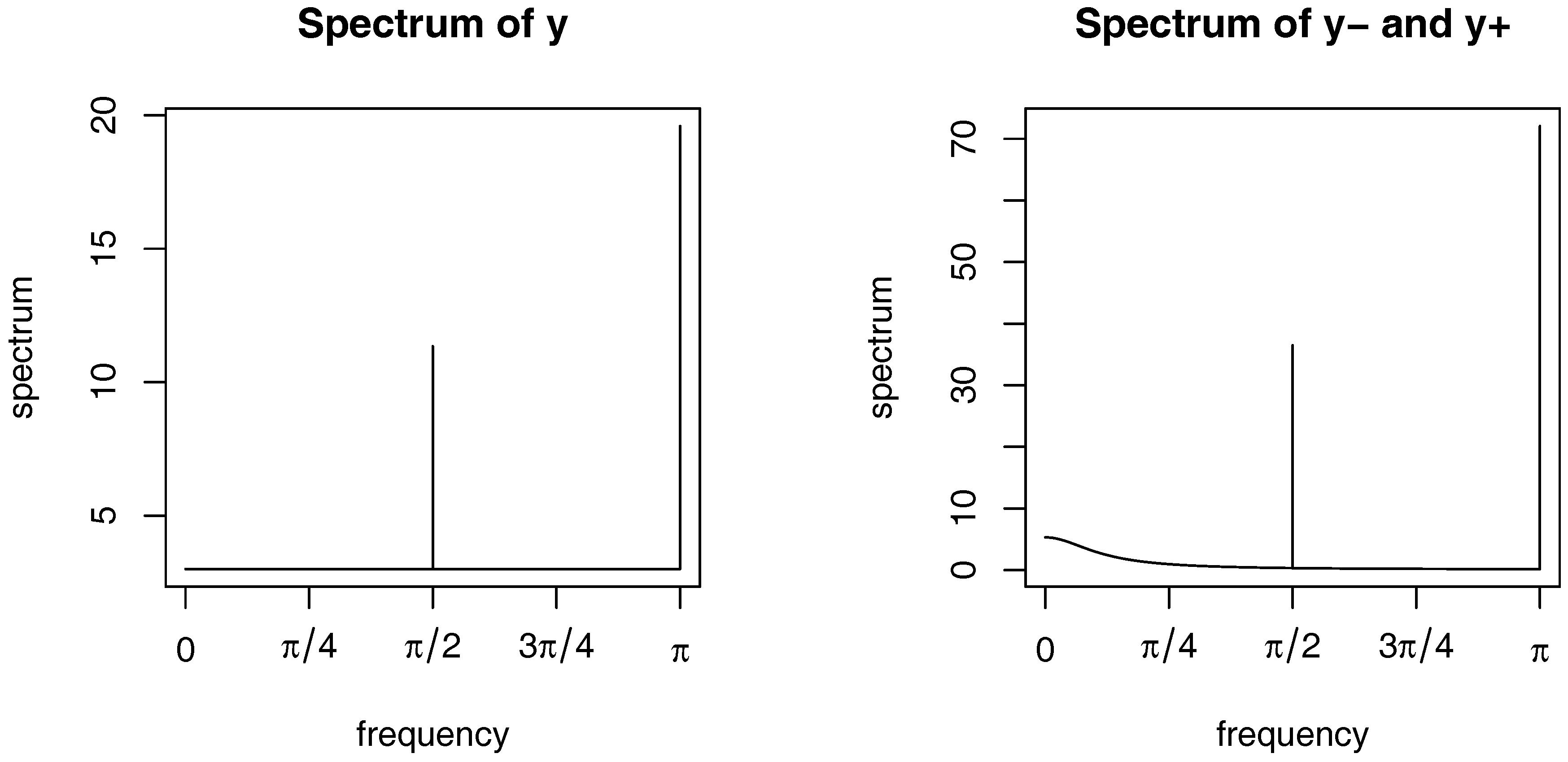
where $D_{s,t}$ $(s=1,\dots ,4)$ are quarterly seasonal dummies with values 1 for the corresponding quarter and zero otherwise. The vector of dummy coefficients is given by $\delta ={[-6,1.5,-0.5,5]}^{\prime }$ and the autoregressive parameters ${\varphi }_1$ and ${\phi }_1$ are set to 0.7. $y_t$ is a strong white noise augmented with deterministic quarterly seasonality. The processes $y_t^{-}$ and $y_t^{+}$ are a causal and noncausal AR(1) respectively, once again augmented with quarterly dummies. For the three processes the error term ${\epsilon }_t$ is $iid$ t-distributed with 3 degrees of freedom.2 The spectra of these processes can be found in Figure 1. It can be observed that there are strong peaks at the frequencies $\omega =\frac{1}{2}\pi$ and $\omega =\pi$, which means that there is strong seasonality present in all data generating processes. The computation of these theoretical spectra can be found in Appendix A.

For each series, we consider two types of seasonal adjustment methods. In the first case, we apply the X-11 linear seasonal filter ${\mathsf{\Psi }}_{X-11}^{SA}(L,L^{-1})$ and perform a model selection on the adjusted series denoted $y_t^{SA},$$y_t^{-,SA}$ and $y_t^{+,SA}$. In the second case, the original variables $y_t,$$y_t^{-}$ and $y_t^{+}$ are regressed on four quarterly deterministic seasonal dummies. Model selection is performed afterwards on the residuals from this regression, denoted as $y_t^D,$$y_t^{-,D}$ and $y_t^{+,D}$. In both cases, the model selection is performed as follows. MAR($r,s$) models are estimated on the seasonally adjusted series by the AML estimator (assuming a Student’s $t-$distribution) as described in Section 2.2, for $r+s=p$ where $p=1,\dots ,4$ (which accounts for a total of fifteen models). We then rely on BIC for selecting the specification that minimizes that criterion. The results for the first case are collected in

Table 2. Frequency (in percentages) with which model is selected (X-11 seasonal adjustment), ${\varphi }_1={\phi }_1=0.7$.

	$\mathit{T}=100$			$\mathit{T}=400$			$\mathit{T}=700$
	${\mathit{y}}_{\mathit{t}}^{\mathit{SA}}$	${\mathit{y}}_{\mathit{t}}^{\mathbf{-}\mathbf{,}\mathit{SA}}$	${\mathit{y}}_{\mathit{t}}^{\mathbf{+}\mathbf{,}\mathit{SA}}$	${\mathit{y}}_{\mathit{t}}^{\mathit{SA}}$	${\mathit{y}}_{\mathit{t}}^{\mathbf{-}\mathbf{,}\mathit{SA}}$	${\mathit{y}}_{\mathit{t}}^{\mathbf{+}\mathbf{,}\mathit{SA}}$	${\mathit{y}}_{\mathit{t}}^{\mathit{SA}}$	${\mathit{y}}_{\mathit{t}}^{\mathbf{-}\mathbf{,}\mathit{SA}}$	${\mathit{y}}_{\mathit{t}}^{\mathbf{+}\mathbf{,}\mathit{SA}}$
MAR(0,0)	75.5	0.0	0.0	19.5	0.0	0.0	1.9	0.0	0.0
MAR(1,0)	6.4	82.1	4.4	4.3	83.1	0.0	0.3	73.8	0.0
MAR(0,1)	5.1	5.4	82.7	3.8	0.0	84.5	0.5	0.0	72.2
MAR(2,0)	0.6	4.1	0.2	0.2	1.8	0.0	0.0	1.9	0.0
MAR(1,1)	0.5	3.2	3.6	0.0	4.4	4.3	0.0	5.2	5.4
MAR(0,2)	0.2	0.4	3.6	0.4	0.0	1.9	0.0	0.0	1.9
MAR(3,0)	0.6	0.8	0.0	0.0	0.6	0.0	0.0	0.2	0.0
MAR(2,1)	0.1	0.3	0.3	0.0	0.2	1.0	0.0	0.0	1.2
MAR(1,2)	0.0	0.0	0.3	0.0	0.4	0.1	0.0	0.6	0.1
MAR(0,3)	0.1	0.0	0.7	0.0	0.0	0.8	0.0	0.0	0.7
MAR(4,0)	4.8	2.6	0.2	38.3	8.3	0.0	50.6	16.9	0.0
MAR(3,1)	0.0	0.2	0.8	0.2	0.0	0.9	0.0	0.0	1.8
MAR(2,2)	0.7	0.3	0.3	0.0	0.0	0.1	0.0	0.1	0.0
MAR(1,3)	0.3	0.3	0.1	0.0	1.2	0.0	0.0	1.3	0.0
MAR(0,4)	5.1	0.3	2.8	33.3	0.0	6.4	46.7	0.0	16.7

and for the second case in Table 4. We display the results for three different sample sizes (T = 100, 400 and 700); 1000 replications are used and we add a burn-in period of 50 observations in both sides to delete the possible effect of initial and terminal values on the simulated series.

4.1.1. Case 1: X-11 Seasonally Adjusted Series

Table 2 reports the frequencies with which BIC selects the different MAR($r,s$) specifications on $y_t^{SA},$$y_t^{-,SA}$ and $y_t^{+,SA}.$ At $T=100$, we see that the percentages with which the correct model is selected lie around 80% for all series. These results are not extremely bad, but relatively low when compared to usual results by BIC. Furthermore, it can be seen that the remaining percentages mostly go to either a MAR($r,s$) of one order higher than the true data generating process or to models with $r+s=4$, where especially the purely causal and noncausal specifications are selected. When T increases, the frequency with which a model of order 4 is selected increases by quite a margin for $y_t^{-,SA}$ and $y_t^{+,SA}$ and drastically for $y_t^{SA}$. The causal and noncausal AR(1) specifications are still selected with percentages ranging from 72% to 85%. However, these frequencies decrease as T increases (despite $T=400$ performing better than $T=100$). For $T=700$, we see that in 97.3% of the cases BIC either selects a MAR(4,0) or MAR(0,4) for $y_t^{SA}$ instead of the correct white noise specification. (Partial) autocorrelation functions are heavily affected, the X-11 filter creates artificial autocorrelation up to order four due to the large weight at that order in the ${\mathsf{\Psi }}_{X_{1}1}^{SA}(L,L^{-1})$ filter. In an almost equal amount of cases, the purely causal MAR(4,0) and purely noncausal MAR(0,4) maximize the log-likelihood (or similarly minimize BIC).

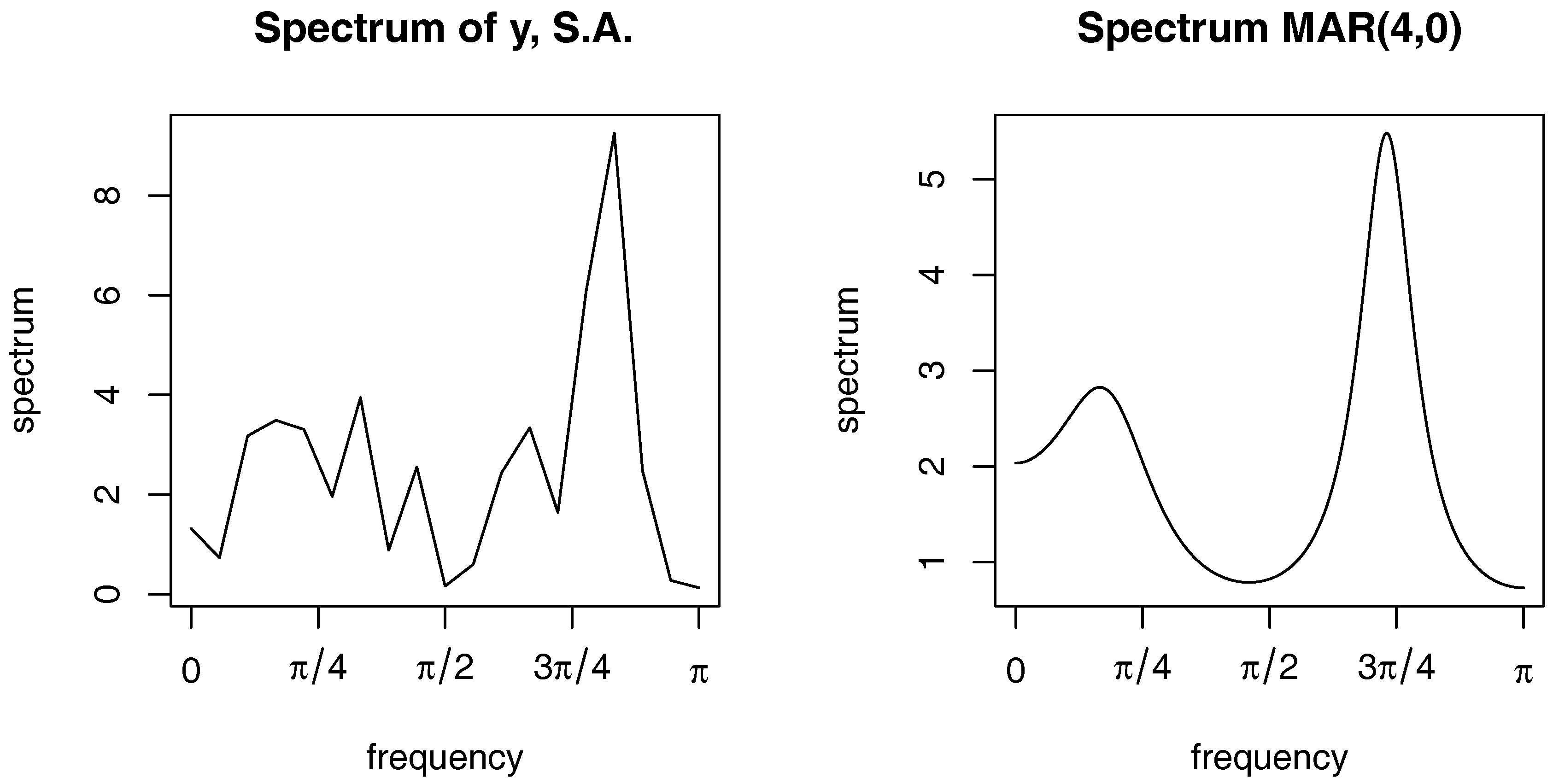
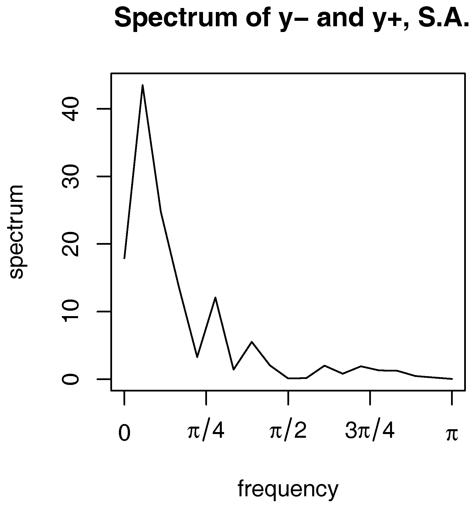
The effect of X-11 seasonal adjustment on a simulated white noise series can be graphically observed in Figure 2a. The graph corresponds to the spectrum of the series, which (roughly said) shows how much a certain frequency contributes to the variance of the series. For example, peaks at frequencies $\omega =0,\pi /2$ and $\pi$ imply that the series contains a trend component and a seasonal component, associated with the once- and twice-a-year frequencies. This is a well-known pattern in quarterly time series data. As we can see in Figure 1a, the process $y_t$ has a flat spectrum (as for white noise every frequency contributes equally to the variance of the series) with peaks at the seasonal frequencies. For $y_t^{SA}$, the peaks at $\omega =0,\pi /2$ and $\pi$ have been deleted as desired. However, we observe that not only the seasonal frequencies are affected and the spectrum coincides more with that of a MAR(4,0) model.3 Kaiser and Maravall (2001) comment on this feature by stating that the X-11 procedure is likely to induce spurious cycles in a white noise series.

For the first-order autoregressive processes, we see a different pattern arising. Since computing spectra is fully based on the autocovariance generating function, one is unable to distinguish between purely causal and noncausal specifications. This means that the spectra of an MAR(1,0) and MAR(0,1) look exactly the same. Hence, Figure 3 shows the spectrum of both the adjusted $y_t^{-}$ and $y_t^{+}$ process. We observe that the X-11 seasonal adjustment filter has affected the spectrum of the series, however only moderately when compared to the white noise case. The time series properties are affected in such a way that higher order models (in particular of order 4) are substantially overselected by BIC, despite the fact that BIC is known for selecting parsimonious models.4 Interestingly, information in other than first and second order moments seems to remain intact, since BIC selects almost only causal [noncausal] models for the seasonally adjusted causal [noncausal] DGP.

This simulation study has also been performed for different values of ${\varphi }_1$ and ${\phi }_1$ and yielded similar results.5 There is, however, one major difference visible. For this reason, we report the results for the case where ${\varphi }_1={\phi }_1=0.3$ in

Table 3. Frequency (in percentages) with which model is selected (X-11 seasonal adjustment), ${\varphi }_1={\phi }_1=0.3$.

	$\mathit{T}=100$			$\mathit{T}=400$			$\mathit{T}=700$
	${\mathit{y}}_{\mathit{t}}^{\mathit{SA}}$	${\mathit{y}}_{\mathit{t}}^{\mathbf{-}\mathbf{,}\mathit{SA}}$	${\mathit{y}}_{\mathit{t}}^{\mathbf{+}\mathbf{,}\mathit{SA}}$	${\mathit{y}}_{\mathit{t}}^{\mathit{SA}}$	${\mathit{y}}_{\mathit{t}}^{\mathbf{-}\mathbf{,}\mathit{SA}}$	${\mathit{y}}_{\mathit{t}}^{\mathbf{+}\mathbf{,}\mathit{SA}}$	${\mathit{y}}_{\mathit{t}}^{\mathit{SA}}$	${\mathit{y}}_{\mathit{t}}^{\mathbf{-}\mathbf{,}\mathit{SA}}$	${\mathit{y}}_{\mathit{t}}^{\mathbf{+}\mathbf{,}\mathit{SA}}$
MAR(0,0)	75.5	1.6	1.3	19.5	0.0	0.0	1.9	0.0	0.0
MAR(1,0)	6.4	73.1	7.9	4.3	58.1	0.4	0.3	25.4	0.0
MAR(0,1)	5.1	9.1	75.8	3.8	0.1	58.5	0.5	0.1	26.6
MAR(2,0)	0.6	2.5	0.5	0.2	1.2	0.0	0.0	0.7	0.0
MAR(1,1)	0.5	1.7	1.8	0.0	2.4	1.4	0.0	1.1	1.0
MAR(0,2)	0.2	0.2	1.3	0.4	0.0	1.3	0.0	0.0	0.6
MAR(3,0)	0.6	0.3	0.1	0.0	0.1	0.0	0.0	0.0	0.0
MAR(2,1)	0.1	0.3	0.2	0.0	0.1	0.4	0.0	0.2	0.4
MAR(1,2)	0.0	0.0	0.0	0.0	0.2	0.2	0.0	0.2	0.0
MAR(0,3)	0.1	0.0	0.4	0.0	0.0	0.1	0.0	0.0	0.0
MAR(4,0)	4.8	7.6	1.9	38.3	36.2	0.6	50.6	71.2	0.2
MAR(3,1)	0.0	0.1	0.4	0.2	0.0	0.7	0.0	0.0	0.5
MAR(2,2)	0.7	0.6	1.1	0.0	0.0	0.0	0.0	0.0	0.0
MAR(1,3)	0.3	0.4	0.0	0.0	0.9	0.0	0.0	0.9	0.1
MAR(0,4)	5.1	2.5	7.3	33.3	0.7	36.4	46.7	0.2	70.6

. Note that the data generating process of $y_t$ (i.e., the static case), does not involve the parameters ${\varphi }_1$ and ${\phi }_1$ and hence the results are identical to those in Table 2. For the two AR(1) processes, we see that also in this case, (non)causality is mostly preserved. The difference, however, lies in the fact that the higher order models are selected more often and faster in this case. For ${\varphi }_1={\phi }_1=0.7$, first order models were selected in approximately 85–90% of the case when $T=100$ and declined to 70–75% when $T=700$. For ${\varphi }_1={\phi }_1=0.3$, first order models are selected in $80-85\%$ when $T=100$ and decline heavily to 25–30% when $T=700$. This is due to the fact that the autoregressive coefficient is relatively low and thus lies much closer to the coefficients of the X-11 filter (see Table 1). Accordingly, the value of the autocovariance at displacement $k=1$ is also lower (in absolute value), which makes it difficult to distinguish it from the autocovariances that are induced by the X-11 filtering process.

4.1.2. Case 2: Deterministic Seasonal Adjustment

If we now use seasonal dummy adjusted variables instead of the seasonal filtered ones, we do not see the patterns of Case 1. In

Table 4. Frequency (in percentages) with which model is selected (no X-11 adjustment), ${\varphi }_1={\phi }_1=0.7$.

	$\mathit{T}=100$			$\mathit{T}=400$			$\mathit{T}=700$
	${\mathit{y}}_{\mathit{t}}^{\mathit{D}}$	${\mathit{y}}_{\mathit{t}}^{\mathbf{-}\mathbf{,}\mathit{D}}$	${\mathit{y}}_{\mathit{t}}^{\mathbf{+}\mathbf{,}\mathit{D}}$	${\mathit{y}}_{\mathit{t}}^{\mathit{D}}$	${\mathit{y}}_{\mathit{t}}^{\mathbf{-}\mathbf{,}\mathit{D}}$	${\mathit{y}}_{\mathit{t}}^{\mathbf{+}\mathbf{,}\mathit{D}}$	${\mathit{y}}_{\mathit{t}}^{\mathit{D}}$	${\mathit{y}}_{\mathit{t}}^{\mathbf{-}\mathbf{,}\mathit{D}}$	${\mathit{y}}_{\mathit{t}}^{\mathbf{+}\mathbf{,}\mathit{D}}$
MAR(0,0)	92.9	0.0	0.0	93.9	0.0	0.0	96.6	0.0	0.0
MAR(1,0)	2.5	89.2	2.9	2.7	95.8	0.0	1.3	96.4	0.0
MAR(0,1)	3.2	3.2	90.3	2.9	0.0	96.4	1.9	0.0	97.3
MAR(2,0)	0.3	3.6	0.1	0.2	2.1	0.0	0.1	1.5	0.0
MAR(1,1)	0.4	2.4	2.4	0.2	1.8	1.8	0.0	1.5	0.7
MAR(0,2)	0.2	0.3	2.7	0.1	0.0	1.6	0.1	0.0	1.8
MAR(3,0)	0.1	0.5	0.0	0.0	0.0	0.0	0.0	0.1	0.0
MAR(2,1)	0.1	0.2	0.5	0.0	0.3	0.1	0.0	0.2	0.0
MAR(1,2)	0.1	0.2	0.3	0.0	0.0	0.1	0.0	0.2	0.0
MAR(0,3)	0.0	0.0	0.4	0.0	0.0	0.0	0.0	0.0	0.2
MAR(4,0)	0.0	0.0	0.0	0.0	0.0	0.0	0.0	0.0	0.0
MAR(3,1)	0.0	0.0	0.1	0.0	0.0	0.0	0.0	0.0	0.0
MAR(2,2)	0.0	0.2	0.1	0.0	0.0	0.0	0.0	0.1	0.0
MAR(1,3)	0.0	0.2	0.1	0.0	0.0	0.0	0.0	0.0	0.0
MAR(0,4)	0.2	0.0	0.1	0.0	0.0	0.0	0.0	0.0	0.0

, the amount of times the correct model is selected is high. Frequencies increase with the number of time observations, making the selection consistent. In the few cases the right model is not selected, the chosen model has at most a single order more than the correct specification. For $y_t^D$ it selects almost equally the MAR(1,0) and MAR(0,1), while for $y_t^{-,D}$ it picks either the causal MAR(2,0) or the MAR(1,1). For $y_t^{+,D}$, the noncausal MAR(0,2) and MAR(1,1) are often the second best choice.

In the light of cases 1 and 2, we conclude that using raw series and exploiting the correct deterministic seasonal features of the series, does not induce spurious dynamics. X-11 type of filters typically create both causal and noncausal autoregressive parts (due to their two-sidedness) especially if they are applied to white noise series. We do, however, not claim that these filters should not be used. The removal of seasonality remains a challenging task. The data generating processes considered here only take into account deterministic seasonality. In case of data containing stochastic seasonality, deterministic terms (like e.g., quarterly dummies) will not capture the true seasonal dynamics (see Bell 1987, for the connection between deterministic and stochastic seasonality).

4.2. Mixed Causal-Noncausal Processes

For the purely causal and noncausal processes, we have seen that X-11 seasonal adjustment might heavily affect model selection. The other seasonal adjustment method, where we use an auxiliary dummy regression to remove the seasonality, does not introduce these side effects. This is of course no surprise, as the seasonality introduced in the DGP is indeed deterministic. For this reason, we only investigate the effects of X-11 seasonal adjustment for mixed causal-noncausal processes. In particular, we consider the following three data generating processes for the stationary time series $y_t^{-},y_t^{+}$ and $y_t$:

$$\begin{array}{cc}\hfill (1-{\varphi }_{1}L)(1-{\phi }_1{L}^{-1})y_t^{}& =\sum _{s=1}^4{\delta }_s{D}_{s,t}+{\epsilon }_t,\hfill \\ \hfill (1-a_{1}L-a_2{L}^2)y_t^{-}& =\sum _{s=1}^4{\delta }_s{D}_{s,t}+{\epsilon }_t,\hfill \\ \hfill (1-b_1{L}^{-1}-b_2{L}^{-2})y_t^{+}& =\sum _{s=1}^4{\delta }_s{D}_{s,t}+{\epsilon }_t.\hfill \end{array}$$

The three processes $y_t,y_t^{-}$ and $y_t^{+}$ are a mixed causal-noncausal MAR(1,1), a causal AR(2) and a noncausal AR(2) process respectively. All processes are augmented with seasonal dummies. Once again, we take the vector of dummy coefficients given by $\delta ={[-6,1.5,-0.5,5]}^{\prime }$ and the error term ${\epsilon }_t$ to be $iid$ t-distributed with 3 degrees of freedom. The autoregressive coefficients are taken as ${[a_1,a_2]}^{\prime }={[b_1,b_2]}^{\prime }={[{\varphi }_1,{\phi }_1]}^{\prime }={[0.3,0.4]}^{\prime }$. The results of the model selection procedure for these processes can be found in

Table 5. Frequency (in percentages) with which model is selected (X-11 seasonal adjustment) for the MAR(1,1), MAR(2,0) and MAR(0,2).

	$\mathit{T}=100$			$\mathit{T}=400$			$\mathit{T}=700$
	${\mathit{y}}_{\mathit{t}}^{\mathit{SA}}$	${\mathit{y}}_{\mathit{t}}^{\mathbf{-}\mathbf{,}\mathit{SA}}$	${\mathit{y}}_{\mathit{t}}^{\mathbf{+}\mathbf{,}\mathit{SA}}$	${\mathit{y}}_{\mathit{t}}^{\mathit{S}\mathit{A}}$	${\mathit{y}}_{\mathit{t}}^{\mathbf{-}\mathbf{,}\mathit{S}\mathit{A}}$	${\mathit{y}}_{\mathit{t}}^{\mathbf{+}\mathbf{,}\mathit{S}\mathit{A}}$	${\mathit{y}}_{\mathit{t}}^{\mathit{SA}}$	${\mathit{y}}_{\mathit{t}}^{\mathbf{-}\mathbf{,}\mathit{SA}}$	${\mathit{y}}_{\mathit{t}}^{\mathbf{+}\mathbf{,}\mathit{SA}}$
MAR(0,0)	0.0	0.0	0.0	0.0	0.0	0.0	0.0	0.0	0.0
MAR(1,0)	9.6	2.2	0.2	0.0	0.0	0.0	0.0	0.0	0.0
MAR(0,1)	18.2	0.4	1.9	0.4	0.0	0.0	0.0	0.0	0.0
MAR(2,0)	2.4	61.7	2.8	0.0	24.5	0.0	0.0	5.0	0.0
MAR(1,1)	57.2	5.0	5.0	92.3	0.0	0.0	90.6	0.0	0.0
MAR(0,2)	4.7	2.2	62.0	0.0	0.0	26.9	0.0	0.0	6.5
MAR(3,0)	0.6	2.3	0.2	0.0	0.2	0.0	0.0	0.1	0.0
MAR(2,1)	1.7	2.8	0.4	3.8	1.5	0.0	5.3	0.6	0.0
MAR(1,2)	2.0	0.7	2.5	2.1	0.0	1.5	3.5	0.0	0.8
MAR(0,3)	0.9	0.1	2.6	0.0	0.0	0.4	0.0	0.0	0.1
MAR(4,0)	0.4	16.8	1.4	0.1	72.9	0.1	0.0	94.1	0.0
MAR(3,1)	0.3	1.4	1.4	0.3	0.5	0.4	0.4	0.1	0.0
MAR(2,2)	0.4	1.0	1.2	0.0	0.3	0.6	0.0	0.1	0.3
MAR(1,3)	0.3	2.1	1.1	0.0	0.1	0.5	0.0	0.0	0.2
MAR(0,4)	1.3	1.3	17.3	0.4	0.0	69.6	0.2	0.0	92.1

.

It can be seen that the results for the causal and noncausal AR(2) are relatively similar to the results found for their AR(1) counterparts in the previous section. That is, as T grows larger, the frequency with which BIC selects an autoregressive model of order 4 increases. For the MAR(1,1), this pattern does not arise. For $T=\{400,700\}$, the MAR(1,1) model is selected in approximately $90\%$ of the cases and thus there is no tendency to select models of order 4. This result seems to suggest that the overselection of models of higher orders does not play a role for the mixed causal-noncausal model. However, if we allow p to take values higher than 4, we see that also in this case, models of higher dynamic orders are selected.

The results for the model selection procedure on the X-11 seasonally adjusted MAR(1,1) process $y_t$ when allowing for a maximum autoregressive order of $p=8$ can be found in

Table 6. Frequency (in percentages) with which model is selected (X-11 seasonal adjustment) for the MAR(1,1).

	$\mathit{T}=100$	$\mathit{T}=400$	$\mathit{T}=700$		$\mathit{T}=100$	$\mathit{T}=400$	$\mathit{T}=700$
MAR(1,0)	8.6	0.0	0.0	MAR(4,2)	1.1	0.5	0.0
MAR(0,1)	11.6	0.0	0.0	MAR(3,3)	0.2	0.0	0.0
MAR(2,0)	1.5	0.0	0.0	MAR(2,4)	1.0	0.3	0.0
MAR(1,1)	36.2	12.2	0.4	MAR(1,5)	4.7	34.5	44.4
MAR(0,2)	3.2	0.0	0.0	MAR(0,6)	1.1	0.2	0.0
MAR(3,0)	0.2	0.0	0.0	MAR(6,1)	0.1	1.7	1.7
MAR(2,1)	0.9	0.1	0.0	MAR(5,2)	0.4	1.8	1.8
MAR(1,2)	3.8	0.7	0.0	MAR(4,3)	0.1	0.3	0.0
MAR(0,3)	1.5	0.0	0.0	MAR(3,4)	0.1	0.1	0.0
MAR(4,0)	0.4	0.0	0.0	MAR(2,5)	0.8	0.5	1.2
MAR(3,1)	0.5	0.0	0.0	MAR(1,6)	1.5	4.4	3.5
MAR(2,2)	0.4	0.0	0.0	MAR(0,7)	0.3	0.0	0.0
MAR(1,3)	0.8	0.0	0.0	MAR(8,0)	0.1	0.0	0.0
MAR(0,4)	0.8	0.0	0.0	MAR(7,1)	0.1	0.0	0.0
MAR(5,0)	1.1	0.0	0.0	MAR(6,2)	0.1	0.0	0.0
MAR(4,1)	3.8	6.6	1.6	MAR(5,3)	0.1	0.1	0.2
MAR(2,3)	0.6	0.1	0.0	MAR(4,4)	0.4	0.0	0.0
MAR(1,4)	5.5	3.2	1.0	MAR(3,5)	0.2	0.1	0.2
MAR(0,5)	1.4	0.2	0.0	MAR(2,6)	0.2	0.0	0.0
MAR(6,0)	0.1	0.0	0.0	MAR(1,7)	1.1	1.4	0.8
MAR(5,1)	2.2	30.6	43.0	MAR(0,8)	1.2	0.4	0.2

.6 For $T=100$, the MAR(1,1) model is selected most of the times, but still only accounts for $36.2\%$ of all cases. The remaining $63.8\%$ is scattered over many alternatives. When T grows, the MAR(1,1) model is selected less often and mostly the MAR(5,1) and MAR(1,5) are chosen. For $T=700$, these two models are selected in $87.4\%$ of the cases. Hence, (non)causality is preserved in the sense that the model selection procedure on a X-11 seasonally adjusted MAR process leads to the selection of models that are also mixed causal-noncausal. This might explain why no models of order 4 were selected in Table 5. The X-11 has a high filter weight at displacement 4. However, as the model selection procedure seems to preserve (non)causality, it will also select a model with at least one lag and one lead. In that case, the only options for $p=4$ are the MAR(3,1), MAR(2,2) and MAR(1,3), which never reach displacement 4 both in its lags or leads. By allowing p to take values up to 8, there are mixed models that can have lag or leads at higher displacements. Since the coefficient at lag/lead 5 in the X-11 filter is the third highest (not taking into account displacement 0), it creates a nonzero autocovariance in the series $y_t^{SA}$ at order 5. When one estimates an autoregressive model on this adjusted series, a coefficient significantly different from zero in both the causal (lag 5) and the noncausal part (lead 5) is detected. Hence, within $p=6$, the model with the highest loglikelihood (similarly, the model that minimizes BIC) will be selected. From the results we can see that the MAR(5,1) and MAR(1,5) are being selected in an almost equal amount of the cases. It is important to note that, if we increase p to take values up to 8 for the purely causal and noncausal data generating processes considered in Section 4.1, most frequency is also assigned to the MAR(5,0) and MAR(0,5) respectively.

One may conclude that the seasonal adjustment methods based on linear filters often increase the dynamic order detected by a model selection procedure based on information criteria. However, as we have seen for the case of an MAR(1,1), this order might not be found when the maximum order p on which the model selection procedure is based is not high enough. Hence, a careful inspection of the residuals of the chosen model is highly advised. Note that this feature does not emerge if we carry out a regression with seasonal dummies before investigating the series.

5. Seasonal Adjustment, Noncausality and Inflation Rates

A justification for modelling inflation with MAR models is given in Lanne and Luoto (2013). They show that the hybrid New Keynesian Phillips Curve (NKPC) in its regression form,

$${\pi }_t={\gamma }_f{\mathbb{E}}_t\left({\pi }_{t+1}\right)+{\gamma }_b{\pi }_{t-1}+\beta x_t+{ϵ}_t,$$

where ${\pi }_t$ denotes inflation, ${\mathbb{E}}_t(·)$ the conditional expectation at time t, $x_t$ a measure for marginal costs and ${ϵ}_t$ an $iid$ error term, can be represented as an MAR($r,s$) model as in (2). More generally, Lanne and Saikkonen (2011) and Gouriéroux et al. (2016) discuss how the mixed causal-noncausal model can constitute a stationary solution to linear rational expectation models.

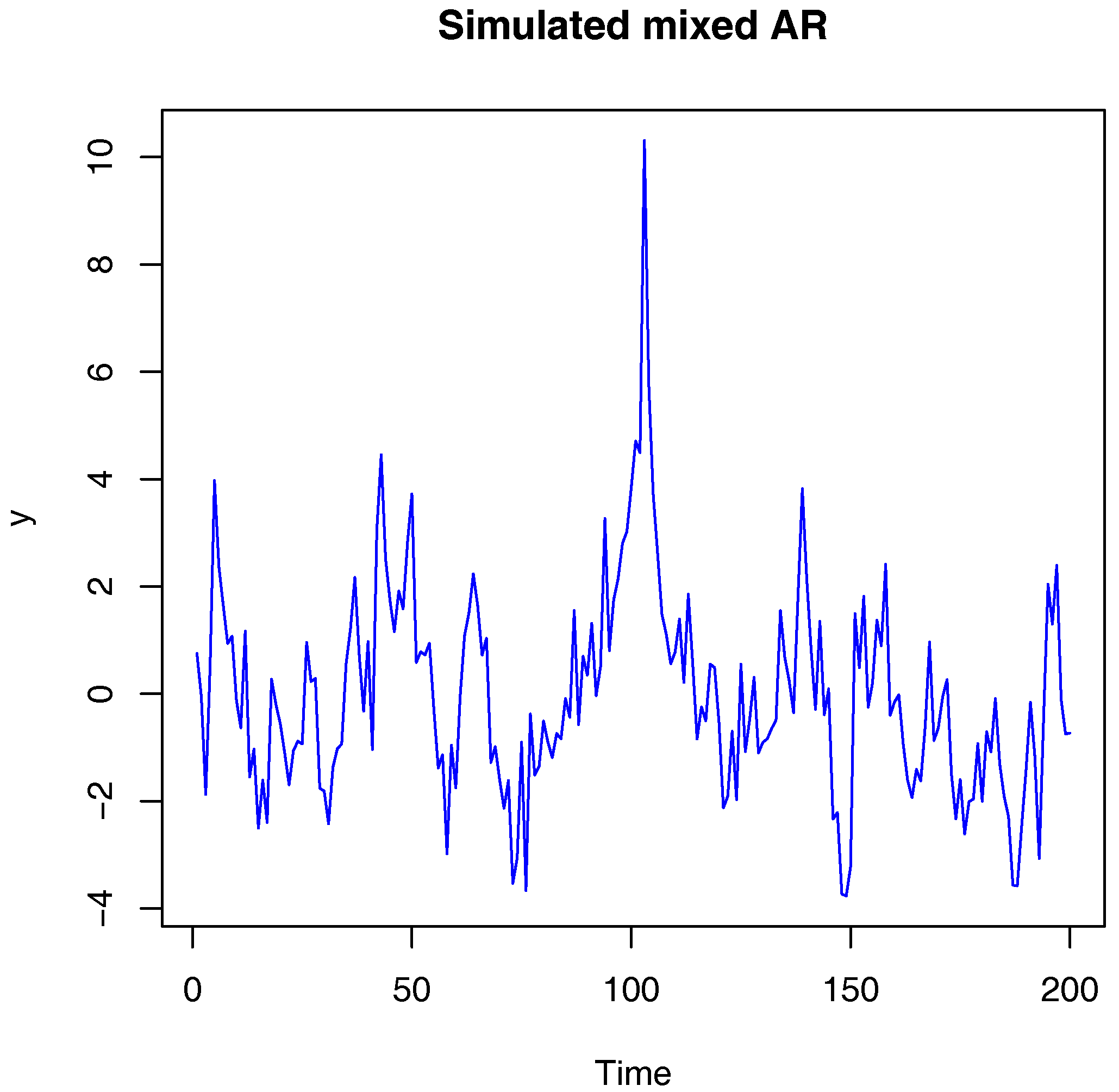
Figure 4 shows a simulated path of an MAR(2,2) with t-distributed error term. It can be seen that such models are able to capture the well-known fluctuating behavior of inflation series. Note that peaks and troughs can be artifically created by considering a more leptokurtic error distribution; choosing the sum of elements in the parameter vector $\mathit{\varphi }$ (respectively $\mathit{\phi }$) close to unity, increases the causal polynomial (respectively noncausal) as driving force in the process.

5.1. Data

We consider Consumer Price Index (CPI) series for the Group of Seven (G7) countries Canada, France, Germany, Italy, Japan, United Kingdom and United States. Raw data are available at the OECD database both at the monthly and quarterly frequency. Despite the fact that quarterly data are directly available at OECD, we do not consider those. The reason for this is that those quarterly observations are computed as the unweighted average over the three months in that quarter. Hence, these data are constructed using a linear filter, which is undesirable in this study as we want to investigate the effect of seasonal adjustment methods based on linear filters. As a consequence, we use quarterly data using point-in-time sampling. That is, we sample the monthly series at the end of each quarter to obtain quarterly data ranging from 1960Q1 until 2017Q2, which accounts for 230 observations. Since prices are stock rather than flow data, this transformation can be considered more natural than averaging.

We examine quarterly observations in order to compare our findings with results found in papers like Lanne and Luoto (2012, 2013) and Lanne et al. (2012a), and in order to make the detection of seasonal unit roots easier. Moreover, X-11 type of filters for monthly data involve a moving average of order 68 and make the identification of the dynamics very difficult, as very large displacements have to be considered. Similar to the simulation study, we investigate series in two ways: seasonality is treated $\left(i\right)$ deterministically or $\left(ii\right)$ by means of seasonal adjustment procedures based on the X-11 filter.

In the first case, we apply a simple seasonal unit root test (HEGY test7, see Hylleberg et al. 1990) on the natural logarithm of the raw prices, i.e.,

$${\mathrm{\Delta }}_4{y}_t=\sum _{s=1}^4{\beta }_s{D}_{s,t}+\gamma T_t+{\pi }_1{z}_{1,t-1}+{\pi }_2{z}_{2,t-1}+{\pi }_3{z}_{3,t-2}+{\pi }_4{z}_{3,t-1}+\sum _{i=1}^p{\zeta }_i{\mathrm{\Delta }}_4{y}_{t-i}+{\epsilon }_t,$$

where $D_{st}$ are seasonal dummies, $T_t$ is a time trend and ${\mathrm{\Delta }}_4=(1-L^4),$ $z_{1,t}=(1+L+L^2+L^3)y_t,z_{2,t}=-(1-L+L^2-L^3)y_t$ and $z_{3,t}=-(1-L^2)y_t.$ Three test-statistics are computed: $(i$) $H_0:{\pi }_1=0$, unit root at the zero frequency (nonseasonal stochastic trend), $\left(ii\right)$ $H_0:{\pi }_2=0$, this implies two cycles per year, $\left(iii\right)$ $H_0:$ ${\pi }_3={\pi }_4=0$, the series contains roots i and $-i$ (seasonal unit roots at annual frequencies). The following transformations have to be made in order to remove the seasonal and nonseasonal unit roots in $y_t$: $\left(i\right)$ if we fail to reject the null ${\pi }_1=0$, $(1-L)$, $\left(ii\right)$ if ${\pi }_2=0$, $(1+L)$ and $\left(iii\right)$ if ${\pi }_3={\pi }_4=0$, $(1+L^2)$. The resulting transformed series is checked for an additional unit root at the zero frequency by the Augmented Dickey Fuller (ADF) test, where the standard regression equation is augmented with quarterly dummies. This additional step allows to determine the degree of integration of the inflation rate, but should be considered with caution in case of bubbles (see Saikkonen and Sandberg 2016, for more details on testing for a unit root in the presence of noncausality). Since for all seven series, the null hypothesis of a unit root is rejected, there is no need to take an additional first difference. That is, the HEGY transformed series are taken as the measure of inflation that is used for the analysis.

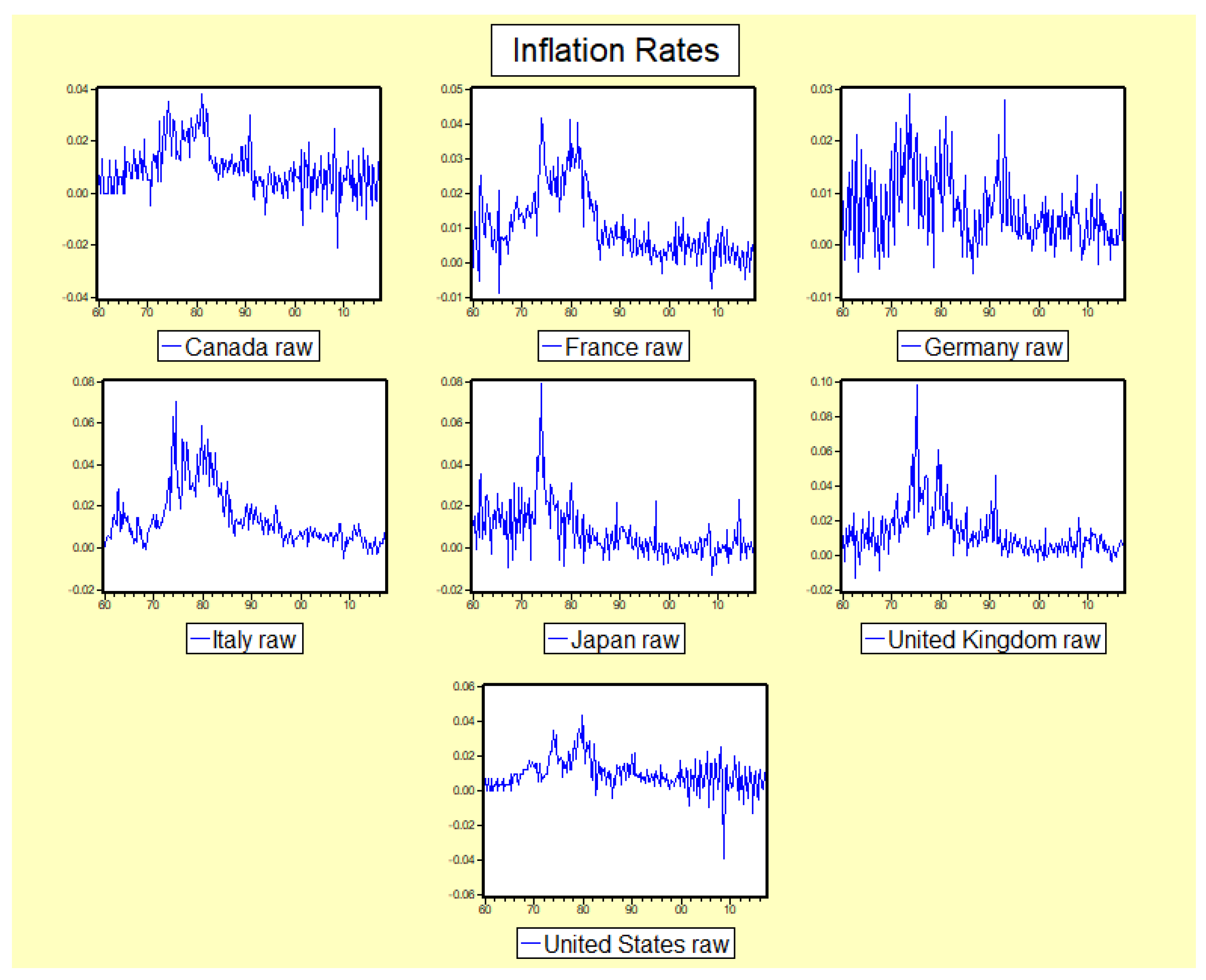
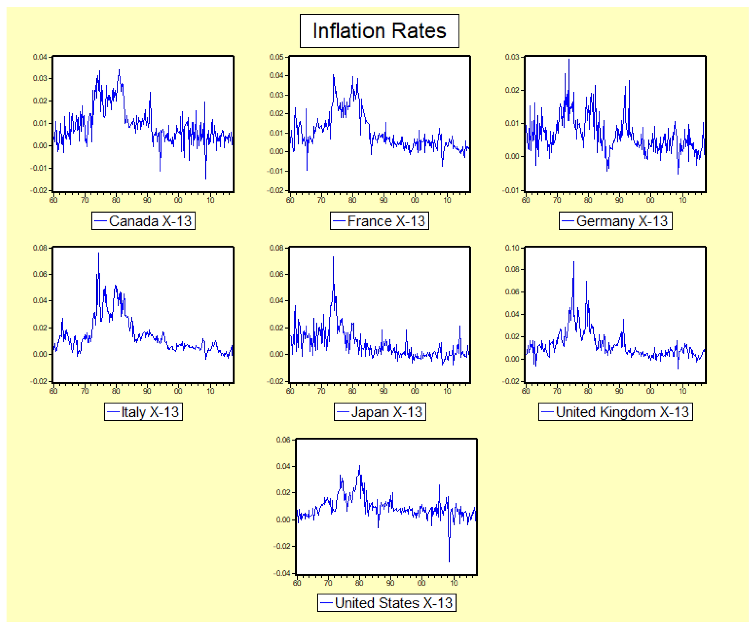
In the second case, the data is immediately adapted by a seasonal adjustment filter. More specifically, we use the X-13 seasonal adjustment procedure on the price series. Afterwards, the conventional ADF test is employed on the log transformed data to check for the presence of a unit root. If this null hypothesis cannot be rejected, the first difference is taken to compute inflation rates. Graphs of these raw and seasonally adjusted series can be found in Appendix B.

After having transformed prices, we apply a model selection procedure using information criteria on both raw and seasonally adjusted inflation series.8 Since mixed causal-noncausal AR processes are not identified by Gaussian likelihood, the first step in modelling a time series with a potential forward-looking component is to check for signs of noncausality. We first estimate pseudo-causal AR(p) models by OLS and choose the model order $p=r+s$ with $p_{\max }=8$ using BIC. Then, diagnostic tests for autocorrelation are performed to see whether additional lags are needed. The null hypothesis of normality is tested on the residuals by means of the Jarque-Bera test.9 In case this null cannot be rejected, there is no need to consider mixed causal-noncausal models, as the backward- and forward-looking components cannot be distinguished from each other. In case the null of normality is rejected, all MAR($r,s$) specifications for the selected pseudo-causal order p are considered. As discussed in Section 2.2, we assume a non-standardized t-distribution for the error process. The model that maximizes the corresponding log-likelihood is chosen to be the final model.

5.2. Results

Table 7. HEGY test on prices and the identification of MAR($r,s$) models on quarterly inflation rates (not s.a.). Rejections of the null hypothesis at a $5\%$ significance level are indicated by asterisks (*).

Country	${\mathit{H}}_0:$ ${\mathit{\pi }}_1=0$	${\mathit{H}}_0:$ ${\mathit{\pi }}_2=0$	${\mathit{H}}_0:$ ${\mathit{\pi }}_3={\mathit{\pi }}_4=0$	Pseudo Model	Jarque-Bera: ${\mathit{H}}_0$: Normality	ARCH-LM: ${\mathit{H}}_0$: no-ARCH	MAR($\mathit{r},\mathit{s}$)
Canada	−0.91	−6.39 *	36.03 *	AR(4)	9.99 *	1.35	MAR(0,4)
France	−1.51	−5.80 *	50.62 *	AR(3)	40.26 *	20.42 *	MAR(3,0)
Germany	−1.05	−5.85 *	27.47 *	AR(4)	6.33 *	1.77	MAR(0,4)
Italy	−0.86	−9.91 *	142.52 *	AR(3)	292.63 *	66.78 *	MAR(3,0)
Japan	−1.29	−3.66 *	25.94 *	AR(4)	121.72 *	10.46 *	MAR(4,0)
United Kingdom	−1.06	−6.21 *	43.70 *	AR(4)	191.87 *	17.06 *	MAR(1,3)
United States	−0.86	−6.60 *	33.44 *	AR(4)	816.86 *	0.82	MAR(2,2)
c.v. (5%)	−3.49	−2.91	6.57		5.99	3.00

shows the results of the HEGY test on the natural logarithm of raw quarterly CPI series. Critical values are from Franses and Hobijn (1997). Test results indicate that the presence of a zero frequency unit root cannot be rejected for all seven countries, while the presence of seasonal unit roots at annual frequencies is rejected in all cases. The possibility of prices containing two cycles per year is rejected for all countries. Hence, $(1-L)$ is the correct transformation to compute inflation for all series. Subsequently, we determine the pseudo-causal model order p, where we include an intercept and quarterly dummies in the regression equation. We find that BIC selects models of order 4 for all countries, except for France and Italy for which a dynamic order of 3 is detected. In all cases, normality of the residuals is rejected using the Jarque-Bera test, which justifies the use of mixed causal-noncausal models. Additionally, all residuals are tested for displaying ARCH effects using Engle’s ARCH[1-2] test. This LM test with the null of no-ARCH is rejected for France, Italy, Japan and the United Kingdom. We discuss this feature and how to deal with it in more detail in Section 5.3. For the p determined in the pseudo-causal model, all MAR($r,s$) models with $p=r+s$ are estimated and the one that maximizes the log-likelihood is the final model chosen. For three countries, a purely causal model is selected, while for two countries a purely noncausal model is chosen as final model. The remaining two countries are found to have mixed causal-noncausal dynamics. The estimated degrees of freedom parameter for the countries Italy, Japan and United Kingdom takes values $1.87,2.14$ and $2.39$ respectively. For the United States and Canada, the values lie slightly higher with 3.47 and 5.79. As shown in Hecq et al. (2016), the estimates are more precise (in finite samples) when the error distribution exhibits fat tails. Hence, the estimation and corresponding identification (through the value of the log-likelihood at the estimated parameter values) is expected to be relatively precise in these cases. For France and Germany, this cannot be argued, as the estimated degrees of freedom parameter takes values 20.22 and 20.40 respectively. Since this distribution approaches the normal distribution, the identification of mixed causal-noncausal models might be problematic (despite the rejection of normally distributed residuals of the pseudo-causal model).

The results for X-13 seasonally adjusted data can be found in

Table 8. Identification of MAR($r,s$) models on quarterly inflation rates (s.a). Rejections of the null hypothesis at a $5\%$ significance level are indicated by asterisks (*).

Country	ADF-Statistic ${\mathit{H}}_0:$ Unit Root	Pseudo Model	Jarque-Bera: ${\mathit{H}}_0$: Normality	ARCH-LM: ${\mathit{H}}_0$: no-ARCH	MAR($\mathit{r},\mathit{s}$)
Canada	$-0.60$	AR(3)	28.11 *	2.39	MAR(0,3)
France	$-0.86$	AR(3)	166.52 *	14.21 *	MAR(3,0)
Germany	$-0.75$	AR(3)	51.33 *	0.22	MAR(0,3)
Italy	$-1.58$	AR(6)	754.96 *	45.54 *	MAR(2,4)
Japan	$-1.55$	AR(3)	76.95 *	23.30 *	MAR(3,0)
United Kingdom	$-0.59$	AR(2)	538.86 *	13.05 *	MAR(0,2)
United States	$-0.54$	AR(3)	1320.34 *	0.64	MAR(0,3)
c.v. (5%)	$-3.43$		5.99	3.00

.10 Note that we do not apply the HEGY test to the seasonally adjusted series, as seasonal effects (and thus also seasonal roots) are assumed to be removed by applying the filters. Hence, it suffices to perform the ADF-test for the log transformed price series. Since all series are found to contain a unit root, we take the first difference $(1-L)$ to compute the growth rate of prices, i.e., inflation. On the transformed series, the pseudo-causal model that adequately captures the serial correlation, is identified. We see that, except for Italy, all countries have an autoregressive order equal to or lower than the one found on raw data. Hence, this is not in line with the results in the simulation study. In all cases, we have the same conclusion for the Jarque-Bera and ARCH-LM test at the 5% significance level when compared to the raw data. That is, the null of normality is rejected for all countries, while the null of no-ARCH effects cannot be rejected for Canada, Germany and the United States. As a result, we can investigate the presence of noncausality. We find that in four out of seven cases, (non)causality is exactly preserved. In these cases, a purely causal [noncausal] model for the raw data series also results in a purely causal [noncausal] model for the seasonally adjusted series. In the other three cases, a mixed causal-noncausal model either switched to a purely causal or noncausal model, or vice versa.

5.3. Considerations

A reason for the different results in the simulation study and the empirical study might be due to the model selection procedure. Gouriéroux and Jasiak (2017) show that the two-step approach, in which the first step consists of estimating purely causal autoregressive processes by OLS, might lead to an estimated model that is misspecified with respect to its noncausal order. A potential other method (henceforth referred to as one-step method) might be to estimate all models directly by means of the method of maximum likelihood, to compute its log-likelihoods and compute information criteria accordingly. However, Gouriéroux and Jasiak (2017) show that this method might also fail to reveal the true causal and noncausal orders. It is important to note that the consequences of an order misspecification in mixed causal-noncausal processes are different from the consequences of order misspecification in Gaussian AR(p) processes. Since Gaussian AR(p) models are nested, a potential wrongly estimated autoregressive order has no effect on the consistency of the autoregressive coefficient estimators. In contrast, mixed causal-noncausal processes with $p=r+s$ with fixed p and varying s are non-nested, and the parameter estimates of the autoregressive coefficients resulting from a misspecified model may be inconsistent. We want to emphasize that the non-nestedness of mixed causal-noncausal processes heavily complicates the model selection procedure. Identification in small samples is achieved faster and more accurate when the processes have extreme fat tails (Hecq et al. 2016). However, as these data have highly nonlinear patterns, we observe that adjusting the sample size by a small number of observations might already have big effects. As the relationships between the causal and noncausal parameters are highly nonlinear and complex, we observe that a slight deviation in (one of) these values might lead to a drastic effect in the maximization of the log-likelihood in finite samples. An additional complication that arises is that optimization routines are sometimes prone to numerical inaccuracies, which amplifies this concern, since they have a direct impact on the final model selected by information criteria.11

Another important consideration is concerned with the type of data considered in this application and its effect on model selection. Inflation rates are relatively volatile and might display conditional heteroskedasticity. Hecq (1996) shows that these effects might directly affect the autoregressive order determined by information criteria. As Gouriéroux and Zakoïan (2016) and Fries and Zakoïan (2017) show, a noncausal Cauchy process can exhibit ARCH-type effects because of its causal recursive double autoregressive structure. Hence, it is advisable to check the residuals of the pseudo-causal model for the presence of ARCH effects in the spirit of misspecification analysis. Cavaliere et al. (2017) propose to use an alternative to the standard Lagrange multiplier test (Engle’s ARCH LM test) as it is based on conventional asymptotic Gaussian p-values, which are not appropriate in this framework. To circumvent this problem, they suggest a test based on Spearman’s rank statistic, which tests non-parametrically the relationship between the residuals and the square of the lagged residuals. Applying this test to the seasonally adjusted data, we fail to reject the null hypothesis of no-ARCH for all series. The test results are however inconclusive, as applying the same test to the residuals of the final chosen MAR($r,s$) model leads to a non-rejection for all countries, except the United Kingdom. One reason for this unexpected result might be that the (potential) ARCH dependence present in the data is not of double autoregressive nature. Another reason might be the fact that we are not dealing with noncausal Cauchy processes (all estimated degrees of freedom parameters are strictly higher than 1) and thus the results found for these processes do not extend to our data. In any case, it seems apparent that the development of more robust strategies for testing misspecification and to perform model selection is needed for mixed causal-noncausal models.

As a last remark, it has to be mentioned that the findings in this paper are likely to extend to cases beyond the exercise of seasonal adjustment. For instance, De Jong and Sakarya (2016) derive a new representation of the Hodrick-Prescott (HP) filter, which highlights that it is a symmetric weighted average similar to the filters considered in this paper. They further state that, in case of a unit root process, the weak dependence of the cyclical component suggests that the unit root is absorbed into the trend component. As the filter (and autocorrelation function) is symmetric, this introduces spurious autocorrelation identically in calendar and reverse time.

6. Conclusions

We investigate the effect of seasonal adjustment on model selection for the inflation rate of the G7 countries. In particular, we study whether seasonal adjustment may spuriously affect the noncausality found in different time series. Since raw data are directly available, we can compare model selection by BIC where one (i) deterministically removes seasonality or ($ii$) applies a predefined seasonal adjustment filter. We find that the linear X-11 seasonal adjustment procedure induces spurious dynamics in white noise processes, which are purely causal or purely noncausal with equal frequency. In case the data generating process is purely causal or noncausal, we find that the direction of causality is preserved after seasonal adjustment. That is, if a process is noncausal the probability to find a purely causal AR model is relatively small. However, we do find that seasonal adjustment decreases the frequency with which we detect dynamics in favor of a less parsimonious model. For both pure processes (causal and noncausal) and mixed causal-noncausal processes, we find that the dynamic order selected after seasonal adjustment is higher than the true autoregressive order of the process.

In the empirical study, we observe that preservation of (non)causality is indeed confirmed in most cases. It is explained how discrepancies might arise due to the presence of ARCH effects and the potential flaws in the model selection procedure due to non-nestedness of mixed causal-noncausal processes. It is, however, very important to carefully consider seasonally adjusted data as it might lead to misleading conclusions. In terms of the hybrid NKPC, identified forward- and backward-looking behaviour might rather be an artefact from the filtering procedure, than a characteristic of the raw data.

References

1. Abeln, Barend, and Jan Jacobs. 2015. Seasonal Adjustment With and Without Revisions: A Comparison of X-13 ARIMA-SEATS and CAMPLET. CAMA Working Papers. Canberra, Australia: Australian National University. [Google Scholar]
2. Alessi, Lucia, Matteo Barigozzi, and Marco Capasso. 2011. Non-Fundamentalness in Structural Econometric Models: A Review. International Statistical Review 79: 1. [Google Scholar] [CrossRef]
3. Bell, William. 1987. A Note on Overdifferencing and the Equivalence of Seasonal Time Series Models with Monthly Means and Models with (0,1,1)12 Seasonal Parts when Θ = 1. Journal of Business and Economic Statistics 5: 383–87. [Google Scholar] [CrossRef]
4. Bell, William, and Steven Hillmer. 2002. Issues Involved with the Seasonal Adjustment of Economic Time Series. Journal of Business & Economic Statistics 20: 98–127. [Google Scholar]
5. Breidt, F. Jay, Richard Davis, Keh-Shin Lii, and Murray Rosenblatt. 1991. Maximum Likelihood Estimation for Noncausal Autoregressive Processes. Journal of Multivariate Analysis 36: 175–98. [Google Scholar] [CrossRef]
6. Brockwell, Peter, and Richard Davis. 1991. Time Series: Theory and Methods, 2nd ed. New York: Springer. [Google Scholar]
7. Cavaliere, Giuseppe, Heino Bohn Nielsen, and Anders Rahbek. 2017. Bootstrapping Non-Causal Autoregressions: with an Application to Explosive Bubble Modelling. Working Paper. Copenhagen, Denmark: University of Copenhagen. [Google Scholar]
8. De Jong, Robert, and Neslihan Sakarya. 2016. The Econometrics of the Hodrick-Prescott Filter. The Review of Economics and Statistics 98: 310–17. [Google Scholar] [CrossRef]
9. Del Barrio Castro, Tomás, and Denise Osborn. 2004. The Consequences of Seasonal Adjustment for Periodic Autoregressive Processes. Econometrics Journal 7: 207–31. [Google Scholar] [CrossRef]
10. Del Barrio Castro, Tomás, Paolo M. M. Rodrigues, and A. M. Robert Taylor. 2017. Semi-Parametric Seasonal Unit Root Tests. Econometric Theory, 1–30. [Google Scholar] [CrossRef]
11. Franses, Philip Hans, and Bart Hobijn. 1997. Critical Values for Unit Root Tests in Seasonal Time Series. Journal of Applied Statistics 24: 25–47. [Google Scholar] [CrossRef] [Green Version]
12. Fries, Sébastien, and Jean-Michel Zakoïan. 2017. Mixed Causal-Noncausal AR Processes and the Modelling of Explosive Bubbles. MPRA Paper 81345. Munich, Germany: University Library of Munich. [Google Scholar]
13. Ghysels, Eric. 1990. Unit Root Tests and the Statistical Pitfalls of Seasonal Adjustment: The Case of U.S. Post War Real GNP. Journal of Business and Economic Statistics 8: 145–52. [Google Scholar]
14. Ghysels, Eric, Hahn S. Lee, and Pierre L. Siklos. 1993. On the (Mis)specification of Seasonality and its Consequences: An Empirical Investigation with U.S. Data. Empirical Economics 18: 191–204. [Google Scholar] [CrossRef]
15. Ghysels, Eric, and Perron Pierre. 1993. The Effect of Seasonal Adjustment Filters on Tests for a Unit Root. Journal of Econometrics 55: 57–98. [Google Scholar] [CrossRef]
16. Gouriéroux, Christian, and Joann Jasiak. 2017. Misspecification of Noncausal Order in Autoregressive Processes. Journal of Econometrics. forthcoming. [Google Scholar]
17. Gouriéroux, Christian, Joann Jasiak, and Alain Monfort. 2016. Stationary Bubble Equilibria in Rational Expectation Models. CRESTWorking Paper. Paris, France: Centre de Recherche en Economie et Statistique. [Google Scholar]
18. Gouriéroux, Christian, and Jean-Michel Zakoïan. 2016. Local Explosion Modelling by Noncausal Process. Journal of the Royal Statistical Society, Series B. [Google Scholar] [CrossRef]
19. Hamilton, James D. 1994. Time Series Analysis. Princeton: Princeton University Press. [Google Scholar]
20. Hecq, Alain. 1996. IGARCH Effects on Autoregressive Lag Length Selection and Causality Tests. Applied Economic Letters 3: 317–23. [Google Scholar] [CrossRef]
21. Hecq, Alain, Lenard Lieb, and Sean Telg. 2016. Identification of Mixed Causal-Noncausal Models in Finite Samples. Annals of Economics and Statistics 123/124: 307–31. [Google Scholar]
22. Hecq, Alain, Lenard Lieb, and Sean Telg. 2017. Simulation, Estimation and Selection of Mixed Causal-Noncausal Autoregressive Models: The MARX Package. Working Paper. Available online: https://ssrn.com/abstract=3015797 (accessed on 8 October 2017).
23. Hylleberg, Svend, Robert F. Engle, Clive W.J. Granger, and Byung Sam Yoo. 1990. Seasonal Integration and Cointegration. Journal of Econometrics 44: 215–38. [Google Scholar] [CrossRef]
24. Kaiser, Regina, and Agustin Maravall. 2001. Measuring Business Cycles in Economic Time Series. New York: Springer. [Google Scholar]
25. Lanne, Markku, and Jani Luoto. 2012. Has U.S. Inflation Really Become Harder To Forecast? Economics Letters 155: 383–86. [Google Scholar] [CrossRef] [Green Version]
26. Lanne, Markku, and Jani Luoto. 2013. Autoregression-Based Estimation of the New Keynesian Phillips Curve. Journal of Economic Dynamics & Control 37: 561–70. [Google Scholar]
27. Lanne, Markku, Janni Luoto, and Pentti Saikkonen. 2012a. Optimal Forecasting of Noncausal Autoregressive Time Series. International Journal of Forecasting 28: 623–31. [Google Scholar] [CrossRef]
28. Lanne, Markku, Henri Nyberg, and Erkka Saarinen. 2012b. Does Noncausality Help in Forecasting Economic Time Series? Economics Bulletin 32: 2849–59. [Google Scholar]
29. Lanne, Marrku, and Pentti Saikkonen. 2011. Noncausal Autoregressions for Economic Time Series. Journal of Time Series Econometrics 3. [Google Scholar] [CrossRef] [Green Version]
30. Maravall, Agustin. 1993. Stochastic linear trends, models and estimators. Journal of Econometrics 56: 5–37. [Google Scholar] [CrossRef]
31. Maravall, Agustin. 1997. Use and (Mostly) Abuse of Time Series Techniques in Economic Analysis. Paper Presented at the 5th CEMAPRE Conference, Lisbon, Portugal, May 26–28. [Google Scholar]
32. Maravall, Agustin. 2006. An Application of the TRAMO-SEATS Automatic Procedure; Direct Versus Indirect Adjustment. Computational Statistics & Data Analysis 50: 2167–90. [Google Scholar]
33. Nelson, Charles, and Heejoon Kang. 1981. Spurious Periodicity in Inappropriately Detrended Time Series. Econometrica 49: 741–51. [Google Scholar] [CrossRef]
34. Saikkonen, Pentti, and Rickard Sandberg. 2016. Testing for a Unit Root in Noncausal Autoregressive Models. Journal of Time Series Analysis 37: 99–125. [Google Scholar] [CrossRef]
35. Wei, William W. S. 2006. Time Series Analysis. Boston: Pearson Addison Wesley. [Google Scholar]
1.
The term ‘approximate’ stems from the fact that the sample used in the likelihood contains only T ( r + s ) terms. As shown in Breidt et al. (1991), this quantity is only an approximation of the true joint density of the data vector y = ( y 1 , , y T ) .
2.
Taking degrees of freedom equal to 1,2,...,5 give similar qualitative results. As shown in Hecq et al. (2016), identification in finite samples becomes more difficult when the degrees of freedom parameter is high. In practice, a value around 10 might already be considered troublesome.
3.
The height of the peaks in this theoretical spectrum can be controlled by adjusting the autoregressive parameters. Here we chose ϕ = [ 0.05 , 0.10 , 0.25 , 0.30 ] to obtain a spectrum similar to the process y t S A .
4.
The same simulation exercise has been done based on a seasonal adjustment method called CAMPLET (see Abeln and Jacobs 2015), which is not based on linear filters. Results show that MAR( r , s ) with r + s = 4 are selected in most of the cases. Causality and noncausality is mostly preserved, but not to the same extent as for the X-11. Results are available upon request.
5.
Simulation results are available upon request.
6.
In order to conserve space, we only report the models that were selected at least once for any T = { 100 , 400 , 700 } .
7.
Alternatively, modified ( M ) seasonal unit root tests, see e.g., Del Barrio Castro et al. (2017), could be used. It has been shown that these tests have good finite sample size and power properties. However, as we only apply the seasonal unit root test for illustrative purposes, we restrict ourselves to the original HEGY test.
8.
The R package MARX used in this study is freely available in the CRAN package repository. See Hecq et al. (2017) for instructions on how to use the package.
9.
Since the Jarque-Bera test is based on the sample skewness and kurtosis, which might not exist for fat-tailed processes, we also performed the Kolmogorov-Smirnov and Anderson-Darling test to check for normality. These tests confirmed the reported results for the Jarque-Bera test.
10.
The same investigation has been done using the TRAMO/SEATS seasonal adjustment method (see Maravall 1997) which is merely used by Eurostat. This method is based on unobserved components decomposition but is not free from filters. In particular, a truncated version of the two-sided, centered, symmetric Wiener-Kolmogorov filter is used to estimate the signal in an observed process y t (for more details, see e.g., Maravall 2006). As the results are very similar, we do not report them here.
11.
We performed the one-step method on the raw and seasonally adjusted inflation rates. In many cases, the one- and two-step procedure select the same model. However, the one-step procedure is more sensitive to numerical inaccuracies in the optimization routine, as the number of different models to be estimated heavily increases even when p goes up from e.g., 4 to 8 (from 15 to 45 models). The model selected in the two-step approach is, however, often among the second or third best when ranked by the values of the information criteria. An advantage of the two-step approach is that p is bounded and numerical inaccuracies only play a role for all models estimated within this p.
Figure 1. Spectra of data generating processes y t (left), y t and y t + (right).
Econometrics 05 00048 g001
Figure 2. Spectra of y t seasonally adjusted (left) and an MAR(4,0) process (right).
Econometrics 05 00048 g002
Figure 3. Spectra of y t and y t + seasonally adjusted.
Econometrics 05 00048 g003
Figure 4. Simulated MAR(2,2) process with ϕ = [ 0.2 , 0.3 ] , φ = [ 0.3 , 0.1 ] , ε t t 5 .
Econometrics 05 00048 g004