1. Introduction
Econometrics is a study of good and bad ways to measure economic relations. This paper is about the use of economic theory in such measurements, and about the need for bridge principles in applied econometrics.
1A long time ago in Fahlbeckska Stiftelsen’s
Statsvetenskaplig Tidskrift (1931) [
2] (p. 281), Ragnar Frisch insisted (in my words) that economic statistics and parameter estimates tell us nothing about pertinent economic phenomena unless they are produced and analyzed within an economic-theoretic conceptualization. A few years later (cf. Haavelmo (1944) [
3] (p. 1)), Trygve Haavelmo professed the same idea: “Theoretical models are necessary tools in our attempts to understand and ‘explain’ events in real life. In fact, even a simple description and classification of real phenomena would probably not be possible or feasible without viewing reality through the framework of some scheme conceived a priori.” I grew up with this idea, and I took it to be valid not just in the paradigms of Frisch and Haavelmo’s econometrics but in all of econometrics. Now I am not so sure. The younger generation of econometricians seems to think differently.
1.1. Three Scenarios for Applied Econometrics
The younger generation of econometricians and the members of Frisch and Haavelmo’s paradigms carry out the theory-data confrontation in different ways. Thus, one may envision three abstract scenarios for the empirical analysis of an economic theory. The scenarios differ in the way the researchers in charge view theory and use it in the measurement of economic relations.
In the first scenario the researcher in charge is an econometrician who, like Frisch, has one leg in mathematical economics and the other leg in mathematical statistics. The theory he confronts with data is an axiomatized theory about a few undefined terms that live and function in an imaginary model world. The researcher acknowledges that there is a definite divide between his model world and the world of observations, and that his data need not provide accurate measurements of the undefined terms of his theory.
2 He formulates his theory in a theory universe and uses bridge principles to describe how his theoretical variables are related to his data variables. The theory-data confrontation, then, becomes a triple of two disjoint universes—one for theory and one for data—and a bridge between them. This scenario I take to depict the way
formal econometrics in the tradition of Frisch functions.
In the second scenario the researcher in charge is an econometrician who confronts an abstract theory with data. The theory may be axiomatized or formulated in accordance with the semantic view of theories. In Haavelmo’s treatise the theory is taken to comprise a system of ordinary or functional equations that express definitional identities, technical relations, or relations depicting behavior (Haavelmo (1944) [
3] (p. 2)). The researcher acknowledges the divide between his model world and the world in which his data resides. To overcome the divide, he identifies his theory variables with
true variables in the real world, and he allows the possibility that he might not have accurate observations of all the relevant true variables.
3 Thus in the second scenario there is no need for a bridge between theory and data. The researcher formulates his theory, describes his data, and carries out the empirical analysis in a data universe. To me this scenario pictures the way
present-day econometrics in the tradition of Haavelmo is carried out.
In the third scenario the researcher uses his knowledge of economic theory and the functioning of economic institutions to formulate his econometric model. The model concerns the behaviour of data variables and may account for both errors of observations and errors in equations. Then, the theory-data confrontation is carried out in a data universe, where the researcher formulates his econometric model and carries out the empirical analysis. It differs from the second scenario in that the model is not derived from the theorems of a pertinent economic theory but springs from the imagination of the researcher in charge. I think this must be a description of the way present-day econometrics is carried out by many young econometricians.
1.2. A Significant Contrast
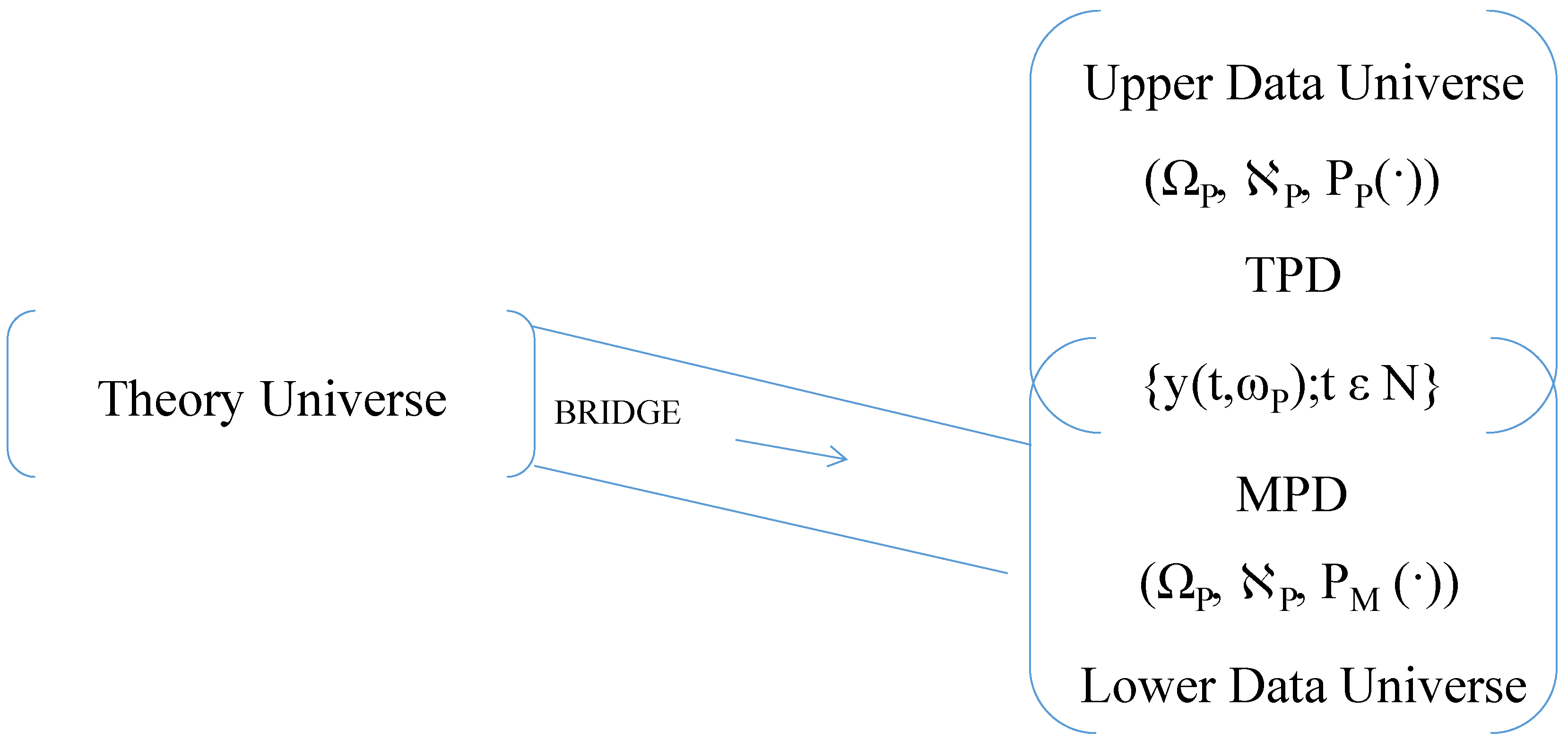
The statistical analyses in the three scenarios differ, and the inferences about social reality that the respective researchers gain from their statistical results also differ. One way to describe the contrast between the empirical analyses in the three scenarios is as follows: The data variables constitute a vector-valued random process, Y = {y(t,ωP); t ε N}, on a probability space, (ΩP, ℵP, PP(·)), where N = {0, 1, 2, …}, ΩP is a subset of a vector space, ℵP is a σ-field of subsets of ΩP, and PP(·):ℵP → [0, 1] is a probability measure. The family of finite-dimensional probability distributions of the members of Y relative to PP(·) is the true probability distribution of the data variables. I denote it by the acronym TPD in which T is short for true, P for probability, and D for distribution. In the last two scenarios the true values of the estimated parameters are taken to be values of pertinent TPD parameters.
The probability distribution that the researcher in the first scenario derives from the probability distribution of his theory variables and the bridge principles is, also, a family of finite-dimensional probability distributions of the members of Y. I denote it by the acronym MPD in which M is short for marginal, P for probability, and D for distribution. With an MPD I can associate a probability measure, PM(·):ℵP → [0, 1], such that Y has the probability distribution MPD relative to PM(∙), and such that Y can be thought of as a vector-valued random process on the probability space, (ΩP, ℵP, PM(·)). In a given theory-data confrontation there may be many MPD distributions. They vary with the models of the theory and the models of the bridge principles. Consequently, parameter estimates in the first scenario are estimates of the parameters of any one of the possible MPD distributions.
1.3. A Figurative Representation of the Contrast
The probability measures, P
P(·) and P
M(∙), are probability measures on one and the same measure space, (Ω
P, ℵ
P). For pedagogical reasons it is useful to think of (Ω
P, ℵ
P, P
P(·)) and (Ω
P, ℵ
P, P
M(·)) as forming part of two different data universes—an upper data universe for (Ω
P, ℵ
P, P
P(·)) and a lower data universe for (Ω
P, ℵ
P, P
M(·)). The picture I have in mind looks roughly like
Figure 1. Here, the bridge connects the theory universe with the lower data universe. The two data universes share the pair, (Ω
P, ℵ
P) and the random process, Y. The probability distribution of Y is TPD in the upper data universe and MPD in the lower data universe. I picture in my mind that present-day econometric analyses in accord with the second or third scenario take place in the upper data universe, while formal-econometric analyses in accord with the first scenario happen in the lower data universe.
1.4. The Preferred Scenario
I believe that Frisch and Haavelmo were right in insisting that economic theory is a necessary tool in a researcher’s attempts to understand and explain the economic phenomena that he observes in social reality. An economic theory is a family of models of a finite number of assertions—axioms—concerning a few undefined terms that live and function in a Frischian model world. As such the theory does not describe behavior and events in real life. Instead it delineates characteristic features of objects and relations in social reality that the originator of the theory has observed. The researcher is to determine when and where the given characteristics have empirical relevance.
The researchers in the three scenarios differ in the way they use theory in their empirical analysis. I have misgivings with the third scenario. The researcher’s cavalier use of theory hampers his ability to give a well-founded analysis of his empirical results. Different theories lead to different interpretations of the results, and the researcher ought to reveal on which theory he bases his analysis. Without such information, meaningful discussions of the researcher’s results become difficult.
I have misgivings with the second scenario, too. An economic theory about behavior or events is a family of models of a finite number of axioms. By identifying theoretical variables with true variables in the real world, and by using his assumptions about the true variables and the data variables to describe properties of the TPD, the researcher in effect treats his theory as if it has only one model. The theory, then, becomes a theory about the characteristics, say, of a representative individual or of a typical strike in the public sector of the economy. Such a theory restricts the kind of inference about social reality that a researcher’s empirical results may confer.
I like the first scenario. In it the researcher’s theory is about the characteristics of behavior and not about the characteristics of a representative individual’s behavior. The statistical analysis confers information about how different the individuals may be for whom the theory is empirically relevant. Similarly, the researcher’s theory about characteristics of events; e.g., strikes in the public sector, is about strikes and not about the typical strike. The statistical analysis confers information about how different the groups that conduct the strikes may be and for which the theory is empirically relevant. Such an empirical analysis is novel both in the way theory is used in the statistical analysis and in the way bridge principles are used to form the inference about social reality that the researcher can derive from his statistical results.
The first scenario is the one I prefer. It ought to appeal to applied econometricians once I have convinced them that there is a way to establish the validity of the bridge principles that are used in an empirical analysis. I hope to do that in
Section 2 of the paper.
2. The Status of Bridge Principles in Applied Econometrics
The bridge principles play three roles in the empirical analysis in the lower data universe. In one role, the bridge principles translate the theory so that it becomes a statement about relations among variables in the data universe. In the second role, the bridge principles convert the probability distributions of variables in the theory universe into a family of probability distributions of variables in the data universe—the MPD—that plays the role of the data generating process in the empirical analysis. In the third role the bridge principles provide the means by which the researcher can identify the empirically relevant models of his theory that his statistical results determine. The three roles of the bridge principles in the lower data universe depict the way theory is incorporated in the empirical analysis of formal econometrics.
Since the MPD may be very different from the pertinent data generating process, the meaningfulness of the empirical analysis in the lower data universe hinges on the validity of the bridge principles. For that reason it is important to search for a general explication of the status of bridge principles in applied econometrics. I will set out to provide such an explication in this section of the paper.
To explicate the status of bridge principles in applied econometrics, I need to explain what I mean by several new concepts: empirical context, empirical relevance, encompassing, congruence, and a data admissible confidence region.
First, empirical context: In the upper data universe in
Figure 1,
the empirical context has two components: (1) axioms and loosely formulated assumptions that the pertinent researcher uses to delineate the characteristics of the data generating process; and (2) the prescriptions that underlie the statistical analysis. The second component details, for example, the way the researcher is to search for a data admissible econometric model that parsimoniously encompasses the so-called local data generating process (cf. Bontemps and Mizon (2003) [
5] (p. 356,359,366) and Hendry and Krolzig (2003) [
6] (p. 380,386–391)).
In the lower data universe in
Figure 1,
the empirical context has, also, two components: (1) the prescriptions that underlie the statistical analysis and (2) a description of the characteristics of a data admissible mathematical model of the MPD. The prescriptions that underlie the statistical analysis detail the way the researcher is to obtain a consistent estimate of a mathematical model of the MPD. Also, a mathematical model of MPD is
data admissible if (1) the estimated mathematical model of MPD satisfies the strictures on which the axioms of the data universe and the prescriptions that underlie the statistical analysis insist; (2) the values that the given model assigns to the parameters of MPD satisfy the strictures on which the theory-axioms, the data-axioms, and the axioms of the bridge insist; and (3) the model lies within a 95% confidence region of the estimated mathematical model of MPD.
Next, empirical relevance: in the upper data universe in
Figure 1 the empirical relevance of a theoretical hypothesis is determined the way the validity of a null hypothesis is decided in mathematical statistics. Specifically, the theoretical hypothesis is judged to be empirically relevant in a given empirical context if and only if it cannot be rejected. In contrast, in the lower data universe in
Figure 1 a family of models of the theory axioms is
empirically relevant if and only if there is a member of the given family which—together with a model of the data axioms and the bridge principles—induces a model of the MPD that belongs to a 95% confidence band of a meaningful statistical estimate of the MPD.
Then, three different concepts of encompassing: exact encompassing, encompassing in the upper data universe, and encompassing in the lower data universe.
Roughly speaking, an econometric model is said to
encompass another econometric model if it can account for the results obtained by the latter (cf. Mizon (1984) [
7] and Hendry and Richard (1989) [
8]). My discussion of encompassing is designed to exhibit the characteristics of the three concepts of encompassing as simply as possible. I consider only cases of parametric encompassing. Also, I adopt the simplest version of the many binding functions that appear in articles on encompassing; e.g., in Gourieroux et al. (1983) [
9], Mizon (1984) [
7], and Florens et al. (1996) [
10]. Finally, since I have had little to say about Bayesian econometrics in the paper, I do not discuss Bayesian ideas of encompassing here. For a comprehensive survey of the development of the encompassing principle in econometrics, the interested reader is referred to Bontemps and Mizon’s (2008) [
11] article on “Encompassing: Concepts and Implementation”.
I will discuss the problem of encompassing within the confines of some given formal theory data confrontation as depicted in
Figure 1. Hence, I am discussing cases in which there is one measurable space, (Ω
P, ℵ
P), with many different probability measures. I also presume that I am considering the probability distribution of a random vector, y(∙), relative to the given probability measures. The distribution of y(∙) relative to P
P(∙) is the TPD distribution of y(∙). Relative to a particular P
M(∙) the distribution of y(∙) is the MPD distribution corresponding to P
M(∙). I will denote a vector of parameters of the TPD distribution of y(∙) by θ
P and any one of the theoretically possible vectors of parameters of the MPD distribution of y(∙) by θ
M. Also, I will denote an econometric model of MPD by a pair, (M1, θ
M°(∙)) and an econometric model of TPD by a pair, (M2, θ
P°(∙)), where, M1 and M2 , and θ
M°(∙), and θ
P°(∙) are two probability distributions and two estimators of θ
M and θ
P, respectively. Finally, I will let s
n denote a finite sample, y
1, …, y
n, of observations of y(∙).
The fact that there is one true TPD and many “true” MPDs has one particularly important implication: The estimator in an econometric model of the TPD is an estimator of the ”true” value of a pertinent TPD parameter. In contrast, the estimator in an econometric model of the MPD is an estimator of the value of an MPD parameter of any one of the possible mathematical models of the MPD. In different words: In an econometric model of the TPD, (M, θP°(∙)), the parameter of M, θP, has a true value. In an econometric model of the MPD, (M, θM°(∙)), the parameter of M, θM, may assume any one of a number of “true” values.
With these remarks in mind I can define the three concepts of encompassing formally as follows:
Definition 1. Suppose that there are three subsets of Rk, ΦP, ΦM, and ΦS, such that θP ε ΦP, θM ε ΦM, and θS ε ΦS. Suppose, also, that I have obtained n independently and identically distributed observations of y, y1, …, yn, and let θP°(∙), θM°(∙), and θS°(∙), respectively, be estimators of θP, θM, and θS in the given sample. Finally, suppose that (M1, θS°(∙)) and (M2, θP°(∙)) are two different econometric models of the TPD, that (M3, θM°(∙)) is an econometric model of the MPD, and that the three estimators are consistent in their respective models. Then,- A.
(M1, θS°(∙)) exactly encompasses (M2, θP°(∙)) in the upper data universe in Figure 1 if and only if there is a binding function, Γ(∙):ΦS → ΦP, such that in M1, the estimates of θP and θS satisfy the equation : θP°(sn) = Γ(θS°(sn)) a.e.. - B.
(M1, θS°(∙)) encompasses (M2, θP°(∙)) in the upper data universe in Figure 1 if and only if there is a binding function, Γ(∙):ΦS → ΦP, such that in M1, Γ(θS0) = plim θP°(sn), and in M2, θP0 = plim θP°(sn), θS0 = plimθS°(sn), and θP0 = Γ(θS0). - C.
(M3, θM°(∙)) encompasses (M2, θP°(∙)) in the lower data universe in Figure 1 if and only if there is a value of θM ε ΦM and a binding function, Γ(∙):ΦM → ΦP, such that in M3, Γ(θM) = plim θP°(sn), and in M2, θP0 = plim θP°(sn), θM0 = plim θM°(sn), and θP0 = Γ(θM0).
In reading this definition there are several things to notice. The definition of exact encompassing is in accord with Definition 1 in Bontemps and Mizon (2008) [
11] (p. 6). Bontemps and Mizon attribute the definition to Florence et al. (1996) [
10]. I have problems with using the definition in the lower data universe for several reasons. Firstly, there need not be a true value of θ
M that I can use to describe the distribution in M1. Secondly, there is no reference to the limiting distributions of the two estimates.
The definition of encompassing in the upper data universe, B, is a rewording of Bontemps and Mizon’s (2003) definition of encompassing (cf. Bontems and Mizon, 2003 [
5] (p. 359)). It is interesting in this context that the definition of encompassing in the lower data universe, C, is a natural extension of definition B. To see why, observe that in M3, θ
M = plim θ
M°(s
n). The required θ
M need not satisfy the equation θ
M = θ
M0. However, if θ
M = θ
M0, (M3, θ
M°(∙)) also encompasses (M2, θ
P°(∙)) in the sense of B. In that sense, C is the natural extension of B to the lower data universe in
Figure 1.
At last I must say what the meanings of congruence and data admissible confidence sets are in the present context. The concept of congruence plays a pivotal role in the LSE methodology. According to Mizon (1995) [
12], in the LSE methodology an econometric model is congruent if it is coherent with a priori theory, coherent with observed sample information, coherent with the measurement system, and encompasses all rival models. For present purposes I will insist on the following modified explication of congruence.
Definition 2. Suppose that there are two subsets of Rk, ΦP and ΦM, such that θP ε ΦP and θM ε ΦM. Suppose, also, that I have n independently and identically distributed observations of y, y1, …, yn, and let θP°(∙) and θM°(∙) be estimators of θP and θM, respectively. Finally, suppose that (M2, θP°(∙)) and (M1, θM°(∙)) are different econometric models of the TPD and the MPD with M2 actually being the TPD, and suppose that the estimators, θP°(∙) and θM°(∙), are consistent in their respective models. Then, (M1, θM°(∙)) is a congruent econometric model of TPD if and only if M1 is coherent with the pertinent a priori theory and (M1, θM°(∙)) encompasses (M2, θP°(∙)) in accord with Definition 1C. The M1 in a congruent econometric model of TPD is termed a congruent model of TPD.
In this definition the a priori theory is a family of models of the axioms of the data universe in a pertinent formal theory-data confrontation. It is, therefore, important to observe that the parameters of M1 in a congruent econometric model of TPD, (M1, θM°(∙)), need not satisfy the conditions of a data admissible mathematical model of the MPD.
Definition 3. Consider a theory-data confrontation in which the sampling scheme that generates the data is adequate. The 95% confidence region around the estimated mathematical model of the MPD is data admissible if it contains both a data admissible mathematical model of the MPD and a congruent model of the TPD.
Theorem 1. Consider one subset of Rk, ΦM, and suppose that θM1 ε ΦM, θM2 ε ΦM, and θM3 ε ΦM are, respectively, parameter vectors of three different models of MPD. Suppose, also, that I have n independently and identically distributed observations of y, y1, …, yn, and let θM°(∙) be an estimator of θM1, θM2, and θM3. Finally, suppose that (M1, θM°(∙)), (M2, θM°(∙)), and (M3, θM°(∙)) are econometric models of the MPD with θM1 being the parameter of M1, θM2 being the parameter of M2, and θM3 being the parameter of M3, and suppose that the estimator, θM°(∙), is consistent in the respective models. If M2 and M3 are data admissible, (M2, θM°(∙)) and (M3, θM°(∙)) encompass each other in accord with Definition 1C. Moreover, if (M1, θM°(∙)) is a congruent econometric model of TPD and M1 is a data admissible model of MPD, (M1, θM°(∙)) encompasses all the econometric models of the MPD, (M, θM°(∙)), with a data admissible mathematical model of MPD, M, and is encompassed by them. However, (M2, θM°(∙)) and (M3, θM°(∙)) need not be congruent econometric models of TPD.
I will sketch a proof of the theorem and leave the missing details to the reader. First let ΦP and ΦM be subsets of Rk, and suppose that the parameter of TPD, θP, belongs to ΦP, and that ΦM, θM1, θM2, and θM3 are as described in the theorem. Also, let θP°(∙) be an estimator of θP, let θM°(∙) be an estimator of the three θMi, i = 1, 2, 3, and assume that the estimators are consistent in their respective models. Finally, let (MP, θP°(∙)) be an econometric model of the TPD. Then observe that if (M1, θM°(∙)) is a congruent econometric model of the TPD, there is a binding function, Γ(∙):ΦM → ΦP, such that in M1 Γ(θM1) = plim θP°(sn), and in MP, θP0 = plim θP°(sn), θM0 = plim θM°(sn), and θP0 = Γ(θM0). Next, observe that if M2 and M3 are data admissible, in M2 θM2 = plim θM°(sn), and in M3, θM3 = plim θM°(sn). Hence with Γ(θ) = θ, (M2, θM°(∙)) encompasses (M3, θM°(∙)) in the sense of Definition 1C. Finally, observe that if (M1, θM°(∙)) is a congruent econometric model of TPD and M1 is data admissible, then (M1, θM°(∙)) encompasses both (M2, θM°(∙)) and (M3, θM°(∙)) in the sense of Definition 1C. However, even though the converse is true, neither (M2, θM°(∙)) nor (M3, θM°(∙)) need be congruent econometric models of TPD.
The preceding theorem allows me to explicate the status of bridge principles in applied econometrics as follows:
The Status of Bridge Principles in Applied Econometrics. Consider a theory-data confrontation like the one pictured in Figure 1. The theory is a non-empty family of models of a finite number of assertions concerning a few undefined terms. The bridge comprises a non-empty family of models of a finite number of assertions—the bridge principles—that relate variables in the theory to variables in the data universe. The data universe is as described in a few assertions that delineate the characteristics of the data generating process—the TPD. Assume (1) that there is an empirically relevant model of the theory, and (2) that each data-admissible model of the MPD singles out an empirically relevant model of the theory. Then, the bridge principles are valid in the Real World if and only if all the econometric models of the MPD, (M, θM°(∙)), with a data-admissible M are congruent econometric models of the TPD.4 I will exemplify the preceding definitions and the status of bridge principles in an empirical analysis of a simultaneous-equations model the idea of which I learned from reading Aris Spanos’ (1989) [
14] and (2012) [
15] deliberations about the legacy of Trygve Haavelmo’s (1944) [
3] treatise “The Probability Approach in Econometrics”.
4. The Two Empirical Analyses
For the two empirical analyses I am to generate 1249 “observations” of ((x, u), y). The components of (x, u) are unobservable. Hence only the sample of ys will be observed. To generate the sample of ys I proceed as follows. I presume that the components of y in the TPD distribution satisfy the equations,
I presume, also, that y
3, y
4, ξ
1, and ξ
2 are distributed independently of each other, and that their distribution is given by the equations,
From these equations and the equations in (12) it follows that the joint probability distribution of y
1 and y
2 is as described in
Table 2. But if that is so, then the means and co-variances of the components of y satisfy the equations:
The corresponding values of ξ
1, and ξ
2 are
With these probabilities and moments in mind I use the PcGive’s uniform random number generator, ranu(), and PcGive to produce the required data and to carry out the statistical analysis (cf. Dornik (2009) [
18] (pp. 158–162) and Dornik and Hendry (2009) [
19]). Specifically, I generate 1249 observations of y
1, y
2, y
3, y
4, ξ
1, and ξ
2 with OxMetrics’ random number generator for the uniform distribution, ranu(). The algebra codes in
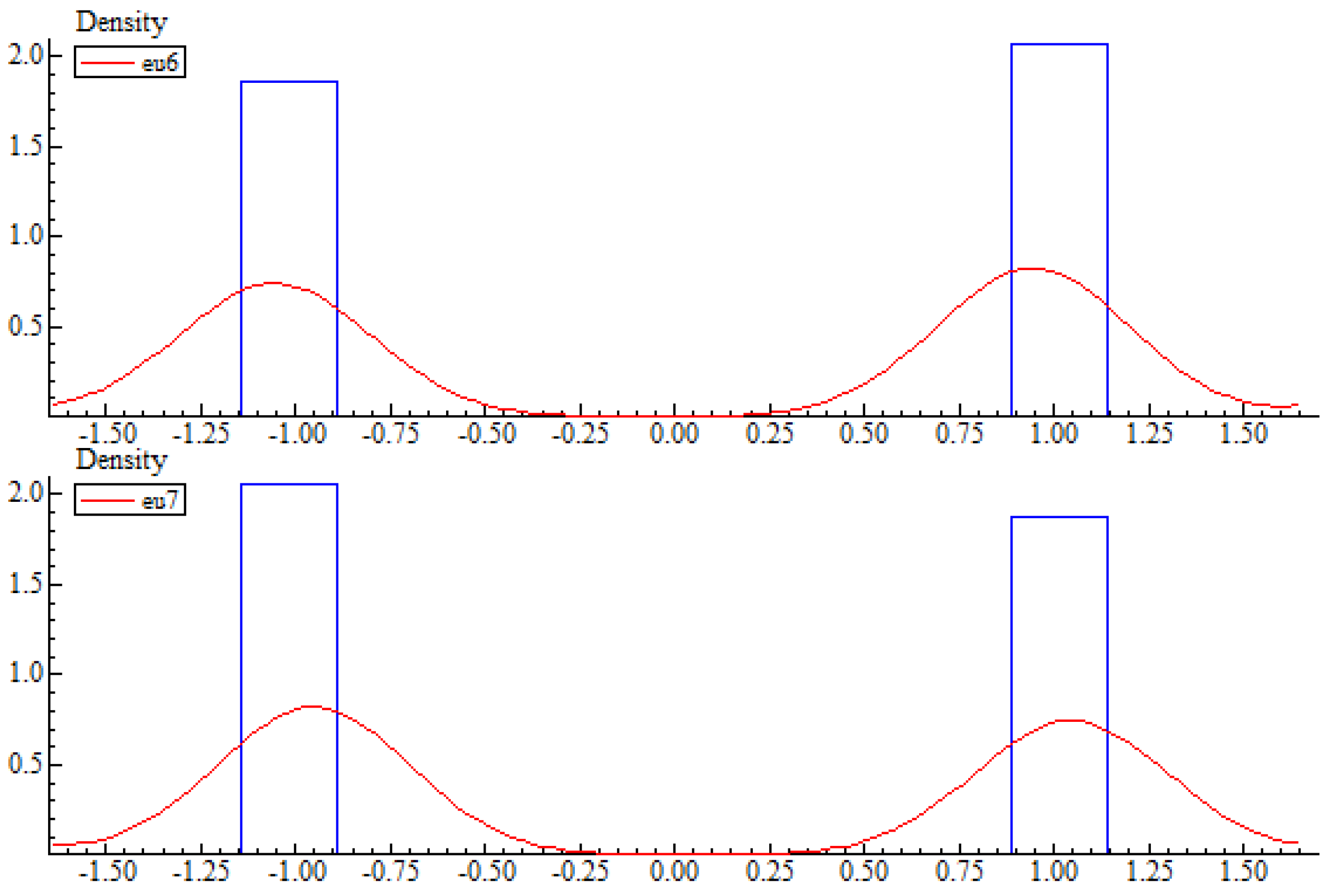
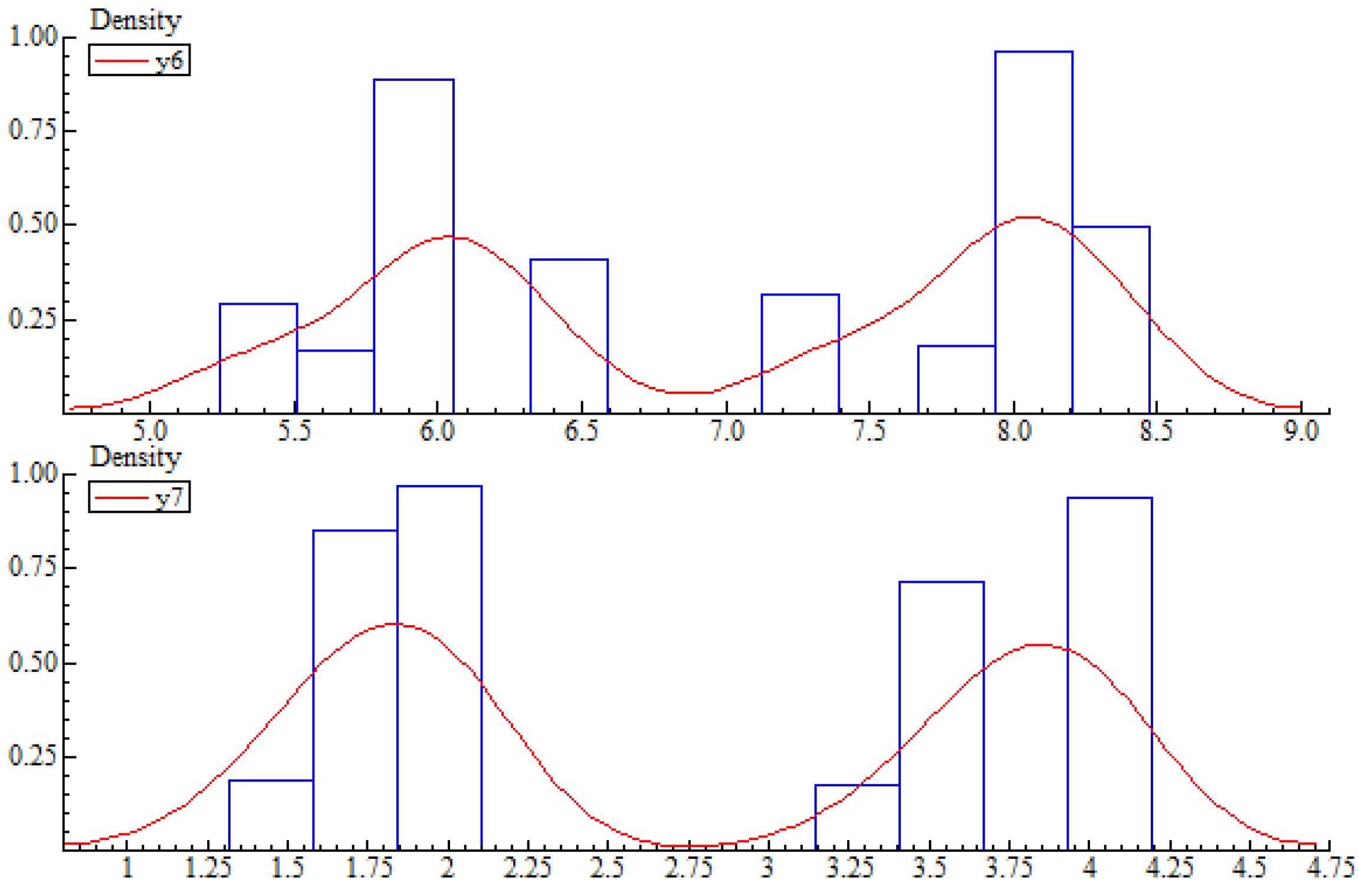
Appendix A detail how the observations were generated. In the printout, y
1 = y6, y
2 = y7, y
3 = y8, y
4 = y9, ξ
1 = u6, and ξ
2 = u7. The results of the statistical analysis are displayed in
Table 3,
Figure 2 and
Figure 3, and
Table A1 and
Table A2 in
Appendix A. They demonstrate that the probability distribution of (y, ξ) described above is statistically adequate in the sense that it accounts for the chance regularities in the data (cf. Spanos (2012) [
15] p. 14).
4.1. An Empirical Analysis in Accord with the Commands of Present-Day Econometrics
In the upper data universe in
Figure 1 the researcher begins by estimating the parameters in Equations (4) and (5). His statistical analysis of the data is centered on three basic ideas: (1) In accord with the commands of present-day econometrics he must obtain consistent estimates of the pertinent TPD parameters; (2) An estimate of the parameters in Equations (4) and (5) is theoretically meaningful if it and Theorem 2 determine an acceptable structural model; (3) An economic theory is taken to be empirically relevant if it—in a standard statistical sense—cannot be rejected. In the present case the theory cannot be rejected only if all the vectors in the confidence region around a given estimate of TPD contains just theoretically meaningful parameter vectors.
The results of the researcher’s statistical analysis are recorded in
Appendix A. The estimated versions of Equations (4) and (5) are as follows:
Except for the normality tests, the diagnostic tests have acceptable results. Also, the sample of ys was obtained with a purely random sampling scheme. This and the fact that the probability distribution of (y, ξ) in (12) is statistically adequate allow the researcher to claim that his parameter estimates are consistent and asymptotically normally distributed.
10The acceptable diagnostic results and the consistency of the researcher’s estimates need not mean that the estimates in (13) and (14) are theoretically meaningful. For an easy check of that, the researcher uses the following inverse of Theorem 2.
Theorem 6. It follows from the equations in Theorem 2 that
From Equations (15) and (16) and the regression results he obtains the following indirect estimates of the structural parameters;
These estimates demonstrate that the parameters in the estimated equations do not constitute parameters of a theoretically meaningful estimate of the TPD.
Since his estimate of TPD is not theoretically meaningful, the researcher finds it interesting to check if there is a parameter vector in Wald’s confidence band that constitutes a parameter vector of a theoretically meaningful estimate of the TPD.
Wald’s confidence band is as described by the following intervals:
In this confidence region the constants in Equations (21) and (22) below constitute, within an admissible margin of error, parameters of a theoretically meaningful estimate of the TPD:
In fact, these two equations and Equations (15) and (16) determine the following values of the structural parameters
The results of the statistical analysis in the upper data universe in
Figure 1 carry three kinds of information: (1) The estimates do not determine theoretically meaningful values of the structural parameters; (2) With 95% probability there exist parameter vectors that satisfy the researcher’s theoretical hypothesis; and (3) Wald’s confidence region contains parameter vectors that do not satisfy the researcher’s theoretical hypothesis. These three observations leave the researcher in the upper data universe with no other choice than to reject the hypothesis which he formulated in the three assumptions he added to Γ
P. i.e., he must conclude that his theory is not empirically relevant.
4.2. A Formal-Econometric Empirical Analysis
In the lower data universe in
Figure 1 the researcher’s empirical deliberations center on three fundamental ideas that describe the prescriptions underlying the statistical analysis, delineate the salient characteristics of a data admissible model of the MPD, and describe what it means for a theory to be empirically relevant. In the present context the prescriptions that underlie the statistical analysis delineate the way the researcher is to obtain a consistent estimate of a mathematical model of the MPD. Also, a mathematical model of the MPD is data admissible if (1) the estimated mathematical model of MPD satisfies the strictures on which the basic-data axioms and the prescriptions that underlie the statistical analysis insist; (2) the values that the given model assigns to the parameters of MPD satisfy the strictures on which the theory axioms and the bridge principles insist; and (3) the model lies within a 95% confidence region of the estimated mathematical model of MPD. Finally, a family of mathematical models of Г
T is empirically relevant if and only if there is at least one member of the family which—with a corresponding model of the axioms of the basic data universe and the Bridge—determines a data-admissible model of the MPD.
The researcher in the lower data universe begins by estimating the parameters in Equations (10) and (11). Since these equations are, formally, like Equations (4) and (5), his estimates are the same as the ones given in Equations (13) and (14). These estimates are not theoretically meaningful. Hence, they cannot be data admissible. Now, the arguments that demonstrate that the parameter values in Equations (21) and (22) are theoretically meaningful suffice to demonstrate that these parameter values are also parameters of a data admissible MPD. Theorem 7 attests to that:
Theorem 7. Suppose that the theory axioms and the axioms of the Bridge are valid. In the present empirical analysis a theoretically meaningful parameter vector whose components belong in Wald’s confidence intervals is the parameter vector of a data admissible MPD distribution of y.
A simple sketch of a proof runs as follows. Let G be a theoretically meaningful parameter vector whose components belong in Wald’s confidence intervals, let H be the structural parameter vector that it determines, and let Ω(H) be the bridge that H determines. Then, define v1 and v2 on Ω(H), formulate the pertinent versions of Equations (8) and (9), and pick an RPD distribution of (x4, x5, u1, u2). The Equations (8) and (9), Theorem 4, and the given RPD distribution of (x4, x5, u1, u2) suffice to construct an MPD distribution of (y, v1, v2). This MPD distribution is data admissible, and G is its parameter vector.
The preceding theorem makes it possible to establish the next theorem. Theorem 8 is the fundamental theorem of the formal-econometric analysis of my data.
Theorem 8 Suppose that the theory axioms and the axioms of the Bridge are valid. Then a parameter vector whose components belong in Wald’s confidence intervals determines an empirically relevant model of ГT if and only if it is a theoretically meaningful parameter vector.
It is obvious that the parameter vector of an MPD which an empirically relevant model of Γ
T determines is theoretically meaningful and has components that belong to Wald’s confidence intervals. Hence to establish the theorem it suffices to show that a theoretically meaningful parameter vector whose components belong in Wald’s confidence intervals determines an empirically relevant model of Γ
T. A theoretically meaningful parameter vector determines a model of axioms A1–A4. Also it follows from Theorem 7 that a theoretically meaningful parameter vector whose components belong in Wald’s confidence intervals is the parameter vector of a data admissible MPD. Hence I can conclude the proof by showing that the pertinent data admissible MPD determines a model of an RPD distribution of (x, u). Let the parameter vector in Equations (21) and (22) be the theoretically meaningful vector in question, and let v
1 and v
2 be the random variables that satisfy the equations
Then, pick an ω
P° in the support of the MPD distribution of v
1 and v
2, and let
and
The MPD distribution of the right-hand side of these equations determines an RPD distribution of the left-hand side that has all the required properties; i.e., a probability distribution that is a model of the RPD distribution of (x1, x3, x4, x5, u1, u2). That and the equation x1 = x2 conclude the proof that the theory universe has an empirically relevant model.
The preceding deliberations show that there is at least one empirically relevant model of Г
T. There may be many more. To find out how many more, the researcher will need two more theorems.
Theorem 9. Suppose that the theory axioms and the axioms of the Bridge are valid. Then the subsets of Wald's confidence intervals that contain the data admissible parameter vectors are as described below:
I have obtained these intervals in two steps. First I used the equations in A4 and Theorem 2 to determine the acceptable minimum and maximum values of the pertinent parameters; e.g., 2.666 < a < 6.6667 and 0.3333 < b < 0.6667. Then, I compared these maximum and minimum values with the Wald intervals in Equations (19) and (20) and determined the extent of the asked-for intervals in Equations (27) and (28).
Theorem 10. Suppose that the theory axioms and the axioms of the Bridge are valid. Then the intervals in Equations (27) and (28) imply that the empirically relevant values of the components of (A, B, E) must satisfy the conditions:
Consequently, in the present empirical context not all the models of the theory axioms are empirically relevant.
The intervals in Equation (29) put added restrictions on the values of B, and E. In doing that, Theorem 10 demonstrates that models of the theory with a B € [−2, −1.977552] and/or an E € [1, 1.14781] cannot be empirically relevant. From this the researcher concludes that the inequalities in Equation (29) demonstrate that all the models of the theory axioms with A € [8, 10], B € (÷1.977552, ÷1], C = 1, D = 0, E € (1.14781, 2], and F = 1 are empirically relevant in the present empirical context. Theorem 11 bears witness to that:
Theorem 11. Suppose that the theory axioms and the axioms of the Bridge are valid. Then all the models of the theory axioms with A € [8, 10], B € (−1.977552, −1], C = 1, D = 0, E € (1.14781, 2], and F = 1 are empirically relevant in the present empirical context.
4.3. The Contrasts and the Status of B1–B5
In this Section, I will describe the contrasts between the empirical analyses in the two data universes in
Figure 1 and conclude the example by establishing the status of the bridge principles, B1–B5, in the present theory-data confrontation.
4.3.1. The Contrasts
The three observations which in a nutshell concretize the results of the empirical analysis in the upper data universe, are also observations that the researcher in the lower data universe made. In the upper data universe the second assertion is to no avail for the empirical relevance of the researcher’s hypotheses because he is unable to assign a probability to his observation of the vector in Equations (21) and (22). In the lower data universe the researcher uses the same vector to show that his theory is empirically relevant. In the upper data universe the third observation leaves the researcher with no other choice than to declare that his theory is not empirically relevant. In the lower data universe the researcher uses a similar observation—Theorem 10—to delineate the subfamily of models of his theory that are empirically relevant.
4.3.2. The Status of B1–B5
The bridge principles play a central role in my deliberations in the lower data universe. It is, therefore, right to question the validity of the axioms of the Bridge. In Stigum (2015) [
1], I claimed that there are good reasons to believe in the validity of the bridge principles in the Real World if the 95% confidence region around a meaningful estimate of the pertinent MPD is data admissible. A 95% confidence band is data admissible if it contains a congruent model of the TPD and a data admissible model of the MPD. In this paper, I insist that the bridge principles are valid in the Real World if and only if (1) the MPD in a congruent econometric model of the TPD is data admissible; and (2) all the pairs of econometric models of the MPD, (M1, θ
M°(∙)) with a data-admissible model of the MPD, are congruent.
Next I will show that the Wald intervals in the present example constitute a 95% data-admissible confidence region, and that B1–B5 are valid in the Real World. I begin by showing that the Wald intervals contains a model of MPD that is congruent. In this case there are two econometric models to consider, (M1, θM°(∙)) and (M2, θP°(∙)), where M1 is any one of the many MPD distributions, θM°(∙) is the estimator of (a, b, c, α, β, γ, σv12, σv22) in Equations (10) and (11), M2 is the TPD distribution, and θP°(∙) is the estimator of (d, e, f, λ, π, ρ, σξ12, σξ22) in Equations (4) and (5). The estimators are consistent, and in M1 it is a fact that θM°(sn) = θP°(sn) a.e.. Hence, (M1, θM°(∙)) exactly encompasses (M2, θP°(∙)) no matter which one of the possible MPD distributions one chooses for M1. It is, also, the case that if I choose the components of θM1 to have the values ascribed to them in Equations (21) and (22), and if I let θP equal θP0, where θPO = (16/3, 2/3, 1/3, 8/3, 1/3, −1/3, 1, 1), then in M2, plim θP°(sn) = θP0 = plim θM°(sn). Hence, with the given choice of M1, M1 is coherent with the pertinent a priori theory, and (M1, θM°(∙)) encompasses (M2, θP°(∙)) in the sense of Definition 1C. Since the sampling system in the present case is adequate, it follows that with the given choice of θM, (M1, θM°(∙)) is a congruent econometric model of the TPD.
At last, I must show that the Wald intervals constitute a data-admissible confidence region and that B1–B5 are valid in the real world. I have shown before that the M1 in the congruent model of TPD is data admissible. Hence, the Wald intervals constitute a data-admissible confidence region. It is, also, obvious from my deliberation above that I can substitute for M1 any data admissible model of MPD and obtain a congruent model of TPD. Hence all the data-admissible models of MPD are congruent. But, if that is true, then it is a fact that the bridge principles in the present example are valid in the real world.


