The First-Exposure Effect in Social Programs: Evidence Against a Welfare Trap

Abstract

We develop a framework for estimating a first-exposure effect (FEE) in a social program, defined as the difference between observed use and the counterfactual use absent any learning from first exposure. In administrative data, those never exposed are unobserved, so the counterfactual distribution must be recovered structurally. Under (i) no state dependence in the counterfactual and (ii) behavioural change only at first use, the observed distribution is a one-altered version of the counterfactual. We derive FEE and marginal FEEs for common count processes, provide an R package fee for estimation, and illustrate with Ontario social assistance data. Results show a 12% reduction in unemployment spells due to first exposure, rejecting the welfare trap hypothesis.

1. Introduction

The perception of a “welfare trap,” where receiving welfare causes an increased probability of receiving future welfare, has long pervaded discussions on welfare programs. Plant (1984) writes that some believe that “social welfare programs create their own dependence,” but finds that evidence pointing towards a welfare trap is weak at best. Levine and Zimmerman (1996) investigate the welfare trap as a mechanism to explain intergenerational correlation in the welfare program Aid to Families with Dependent Children but also finds limited evidence. Many authors, however, such as Verho et al. (2022), who argue that universal basic income can eliminate welfare traps, regard the “welfare trap” concept as a firmly established feature of the welfare system. We ultimately find evidence against this notion.

The idea that a welfare recipient becomes trapped and experiences more welfare spells begs the question: more relative to whom? In administrative program-use data, individuals enter the dataset only upon their first use of the program, so those who never experience first exposure are absent from the sample. This makes direct comparison to a “never-exposed” group impossible. Identification of the first-exposure effect (FEE) therefore requires a structural approach: we recover the unobserved counterfactual distribution from the observed data by imposing two key assumptions. The first is that there is no state dependence in the counterfactual, meaning that the history of visits would have no impact on future visits; outcomes are independent. The counterfactual individual that we envision is one who experiences unemployment and collects welfare but does not learn from the social program itself. The second key assumption is a first-only effect in the factual distribution, meaning that any behavioural change induced by the program occurs only due to the first visit. No new pertinent additional information that could impact the number of visits is presented to the individual.

We interpret “welfare trap” ideology to be that social programs alter the number of visits that would occur relative to the counterfactual. Individuals experience the program, learn, and gain new information. Behaviour is altered in a way that affects the number of visits that would have otherwise occurred in the absence of the learning event. We assume that information has a behavioural effect after the first visit only, and not subsequently, and is the cornerstone in the identification of the first-exposure effect (FEE). This assumption enables us to express the observed factual distribution as a mixture of the counterfactual distribution, recover both distributions, and estimate their difference.

We formally define the FEE as the difference between what factually happens in the presence of first-exposure, and what counterfactually would have happened if individuals were unresponsive to the information presented at first visit: $\mathbb{E}[y_i-y_i^0]$, where $y_i$ is the observed factual data, and $y_i^0$ is the counterfactual outcome that would occur if the individual were impervious to any kind of learning or information from the first visit. We propose a general class of distributions for $y_i$ and $y_i^0$ and identify and estimate the FEE, as well as the associated marginal effects or policy impacts. Estimation of the FEE and marginal FEE, as well as their standard errors, is accomplished via an accompanying R package (fee version 1.0.0) fee, available on CRAN.

Analysis of welfare recipients has been a prominent research agenda with important policy implications. This research has primarily concentrated on the frequency and duration of welfare spells and the associated characteristics of welfare recipients, the state of the labour market, and the structure of welfare policy. The aim of this literature has been to develop causal inferences regarding the distribution of spells and their length that will assist in the development of more effective policies to shorten welfare spells and reduce welfare recidivism. We draw on this literature in a general way to illustrate our new approach using a large administrative data set on welfare recipients from Ontario.

The literature on duration modelling is vast and has important applications to the duration of welfare spells. A good survey of the literature is Van den Berg (2001). The emphasis is on the explanation of the empirical exit rate and its underlying determinants using mixed proportional hazards models. For example, O’Neill et al. (1987) analyze welfare spell duration for young women under the assumption that exits from welfare depend on superior utility outside welfare, where conditional exit probabilities are estimated by spell year, type of exit (marriage or other) and race for a large number of covariates. They find that most welfare spells end in the first year, but, like much of the literature, they do not analyze repeated spells. There are studies that combine analysis of welfare duration and recidivism (Cao, 1996) and that combine spells to examine total time on welfare and the fraction of total welfare income over a fixed time interval, ignoring spell composition (Gottschalk & Moffitt, 1994), largely to circumvent more complex analysis of duration models with repeated welfare spells. While we focus on the frequency of spells and not explicitly on duration, we employ regressions with a log offset, describing event counts per unit exposure (welfare spells per time off welfare). This creates an equivalence between duration and frequency analysis (Laird & Olivier, 1981).

The literature on the frequency of spells is similarly immense and draws on the econometric modelling of count data. The focus in this literature is explicitly on whether individuals experience a welfare spell and, if so, whether and how often that spell is repeated. While our methodology borrows from some of the standard count data models used in this literature, our innovation is in the use of one-altered count data models, which, to our knowledge, have never been employed in this literature. One-altered count data models have been rather confined to the population size estimation literature (e.g., estimating the number of domestic violence victims, illegal immigrants, or animals that have been captured then recaptured; see Böhning and Friedl (2024) for an overview), where they are typically referred to as “one-inflated models” (although the inflation may be negative and thus one-deflating).

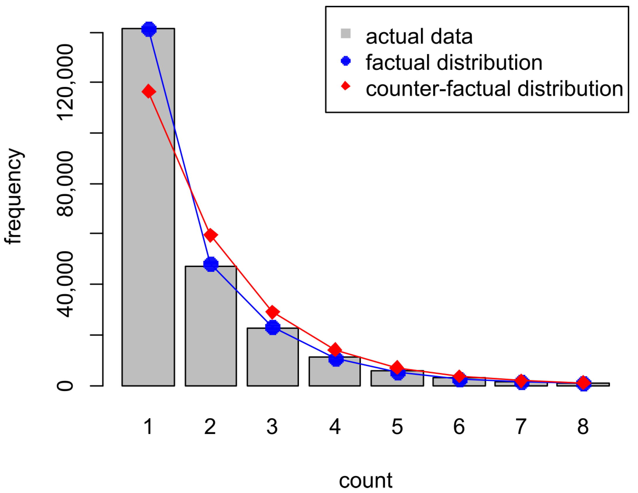
We estimate a FEE in social assistance usage, using monthly data on Ontario Works financial and employment assistance, provided by the Ontario Ministry of Community and Social Services in conjunction with Statistics Canada’s Research Data Centres (Statistics Canada, 2025). Counts of social assistance spells, by individual, are constructed for the 142-month period of observation, resulting in a data set containing 234,320 individuals. The data includes many regressors at the individual level. Social assistance recipients obtain information upon their first exposure that may affect the probability of additional usage. The central tenet of our identification strategy is that all information that may cause a behavioural response is imparted upon the first spell. That is, there is only a first-exposure effect, and no subsequent effects, so the FEE manifests by altering the probability of a single spell. The type of information at first-exposure that we anticipate may invoke a behavioural response that includes (i) learning about one’s preferences towards unemployment, e.g., finding it enjoyable or not; (ii) learning the extent, or lack, of social stigma; (iii) sunk administrative costs, e.g., filling out forms; and (iv) job training that may prevent future unemployment.

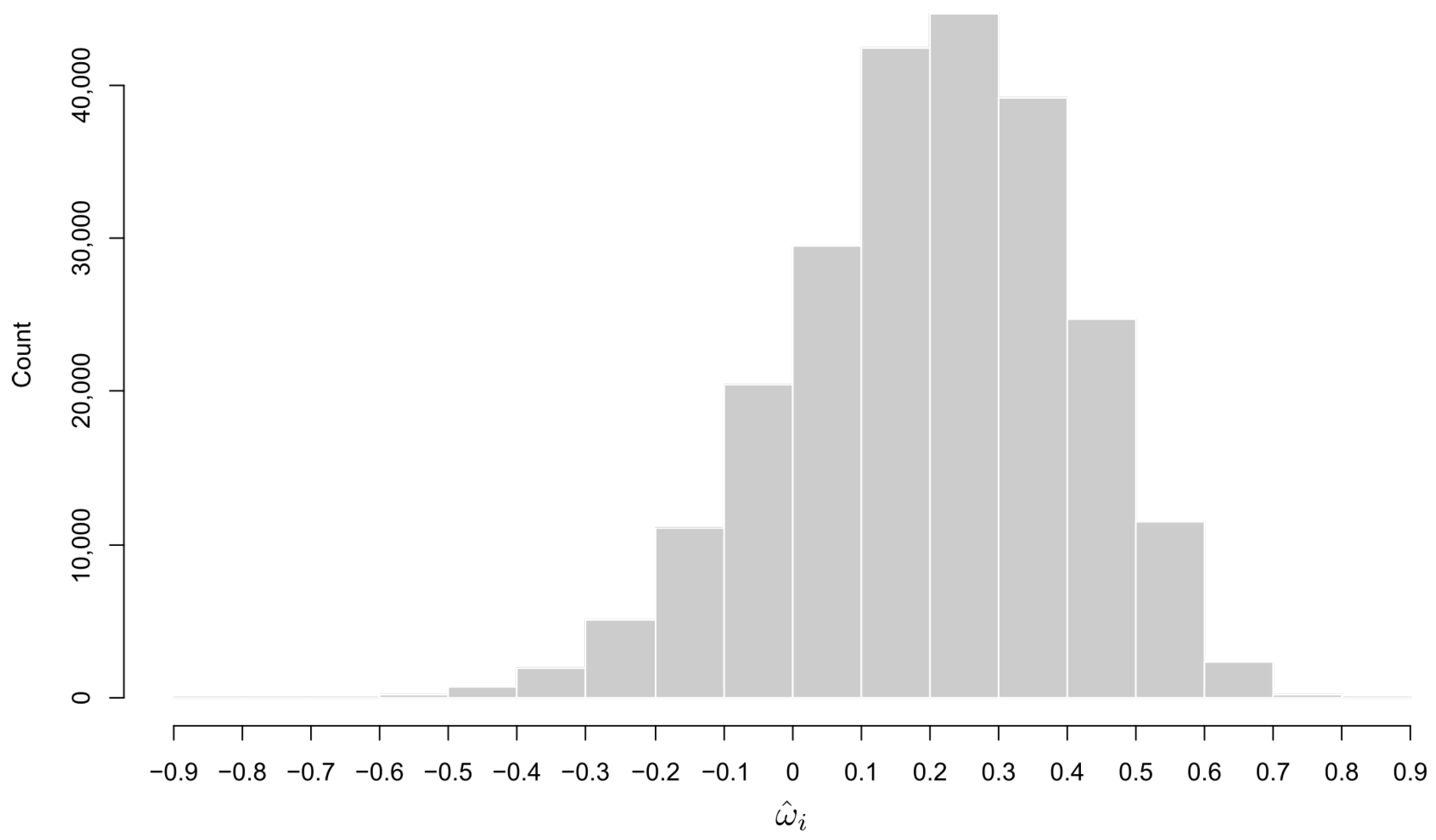
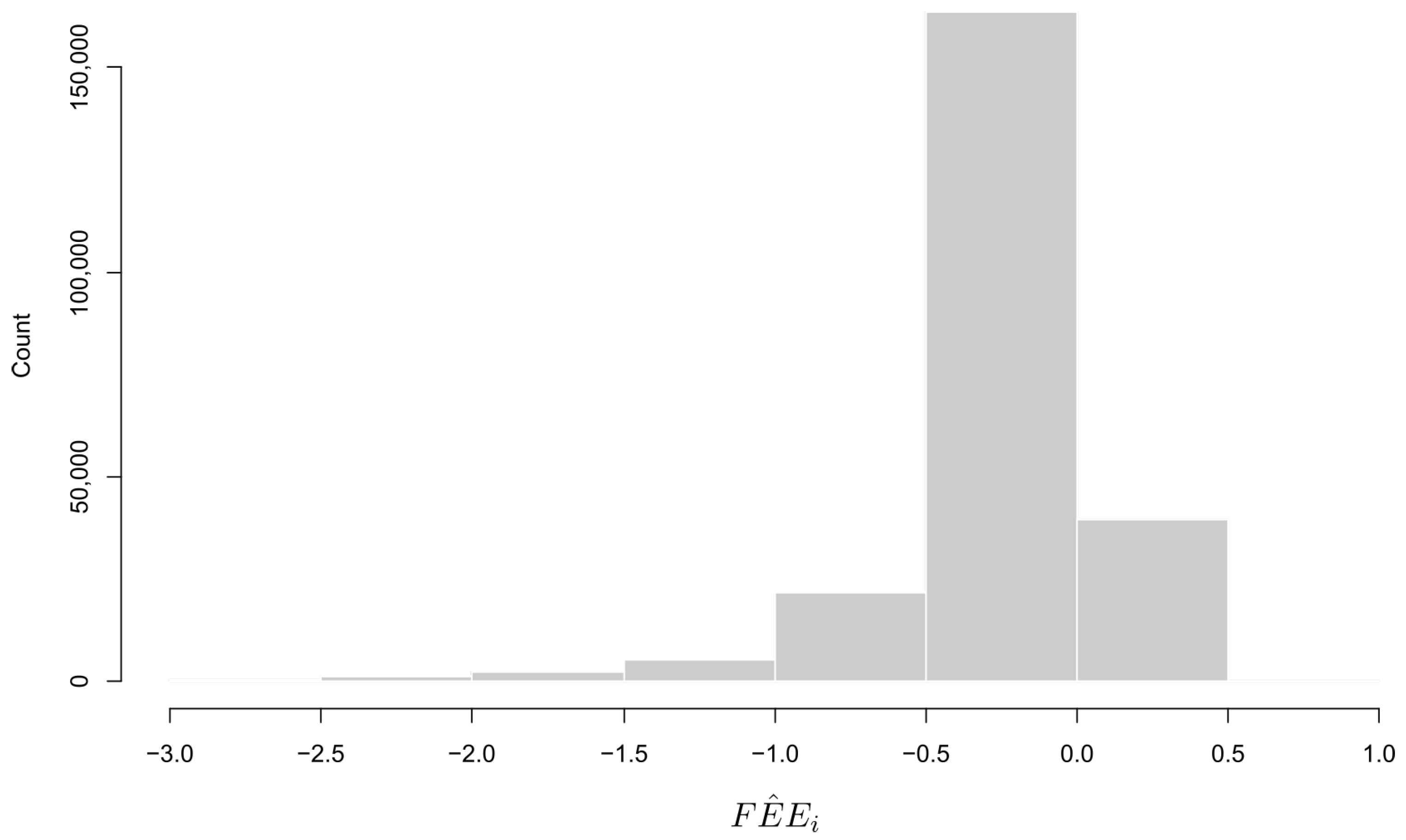
We find that the FEE causes a decrease in social assistance usage on average, contrary to the prediction underlying the welfare trap. We estimate that, on average, individuals experience 0.251 fewer unemployment spells over the period, due to first exposure. This amounts to a reduction in unemployment spells of 12.3%. We estimate marginal effects, finding this reduction in unemployment to be much higher for men. We also find that the deterrence effect of first exposure diminishes as the individual becomes more highly educated, perhaps suggesting a higher ability to anticipate the information that is revealed at first visit.

While we apply our method to social assistance usage, more generally, we have developed a framework for evaluating social programs that are repeatedly used by individuals, where the efficacy of the program depends partly on recidivism, and where policy instruments take effect upon first use. In programs that influence their own use, and where only the first use produces an effect, our framework is appropriate.

2. The First-Exposure Effect

2.1. First-Exposure Effect Defined

The FEE is a comparison of $y_i$ (what factually happened) and $y_i^0$ (what would have happened in the absence of information at first exposure), and is formally defined as

$$FE{E}_i\equiv \mathbb{E}\left[y_i-y_i^0\mid {\mathit{X}}_i,{\mathit{Z}}_i\right],$$

(1)

where ${\mathit{X}}_i$ and ${\mathit{Z}}_i$ are vectors of (possibly identical) regressors; the former affects an underlying counting process and the latter a “one-inflation” component. The estimand in Equation (1) is the expected difference between what is observed and what would be observed in the absence of any learning or information imparted at first exposure. The FEE quantifies the difference in the number of visits to a social program that would have occurred if the experience of the program itself had no impact on the behaviour of the individual. Of further interest will be the “marginal effects”; the dependence of the FEE on a regressor or policy $X_{ij}$ and/or $Z_{ij}$, either ${\displaystyle \frac{\partial FE{E}_i}{\partial X_{ij}}}$ if $X_{ij}$ is continuous or $(FE{E}_i\mid X_{ij}=1)-(FE{E}_i\mid X_{ij}=0)$ if $X_{ij}$ is binary, for example.

2.2. Distribution for $y_i^0$

We propose that $y_i^0$ would follow a known truncated count distribution.

Assumption 1 

(No state dependence in the counterfactual). The distribution for the counterfactual number of visits $y_i^0$ to the social program is

$$y_i^0\sim f^0(y_i^0\mid {\mathit{X}}_i;{\mathit{\theta }}_i);y_i^0=1,2,\dots$$

(2)

where $f^0$ is a zero-truncated counting distribution without state dependence, ${\mathit{X}}_i$ is a vector of regressors, and ${\mathit{\theta }}_i$ is a vector of parameters.

Note that we will suppress the arguments in the notation of the probability functions for brevity; for example, the counterfactual distribution is often denoted as $f^0$.

Assumption 1 is no more restrictive than in any other count data application. The particular distribution for $f^0$ depends on the nature of the data-generating process, but natural a priori choices would be zero-truncated Poisson or zero-truncated negative binomial, which are popular distributions to describe administrative-type data where 0 visits are impossible to observe, and are distributions that invoke an independence assumption. We limit our attention to Poisson and negative binomials; however, our framework can easily be adapted to entertain other counting processes.

2.3. Distribution for $y_i$

In order to identify the causal estimand $FE{E}_i$ in Equation (1), we need to identify the distribution for the observed data, $f\left(y_i\right)$. This relies critically on Assumption 2.

Assumption 2 

(First-only effect). Any behavioural effect from experiencing the social program, relative to the counterfactual, occurs solely due to the first visit.

There is no new information presented at the second, third, etc. visits. Information is absorbed during the first visit and has an effect before the second visit can occur. Provided Assumption 2, any distortion in $f^0$ due to first-exposure manifests at the 1-count. Subsequent visits do not impart additional information capable of altering the number of visits. No new pertinent information is presented, and old information has no new effect. This implies that the factual distribution f is a one-altered version of $f^0$ and that $f\left(y_i\right)$ belongs to a family of one-altered count distributions, several of which have been established (Godwin and Böhning (2017), Godwin (2017), Godwin (2019), and Tajuddin et al. (2022), for example).

Proposition 1 

(Distribution for $y_i$). Provided Assumptions 1 and 2, the observed data $y_i$ follow a one-altered count distribution $f\left(y_i\right)$:

$$\begin{array}{cc}\hfill f\left(y_i\right)& ={\omega }_i+(1-{\omega }_i)f^0\left(y_i\right);y_i=1\hfill \\ \hfill & =(1-{\omega }_i)f^0\left(y_i\right);y_i=2,3,\dots ,\hfill \end{array}$$

(3)

where $f^0$ is truncated Poisson or truncated negative binomial, where ${\omega }_i>0$ corresponds to one-inflation, ${\omega }_i<0$ corresponds to one-deflation, and where ${\omega }_i=0$ corresponds to a standard counting process without alteration at the 1-count.

Proof. 

Assumption 2 implies that first-exposure will add a difference ${\delta }_i$ to the probability of a single visit, relative to the counterfactual

$$f\left(1\right)={\delta }_i+f^0\left(1\right)$$

(4)

but otherwise leave the counterfactual distribution unchanged, at least so that the factual probabilities of visits after the first are proportional to the counterfactual probabilities:

$$f\left(y_i\right)=c_i{f}^0\left(y_i\right);y_i=2,3,\dots ,$$

(5)

where $c_i$ is a proportionality constant and where $c_i>1$ if first-exposure encourages subsequent use, for example. Then, by Equations (4) and (5), a probability mass function for $y_i$ is

$$\begin{array}{cc}\hfill f\left(y_i\right)& ={\delta }_i+f^0\left(y_i\right);y_i=1\hfill \\ \hfill & =c_i{f}^0\left(y_i\right);y_i=2,3,\dots .\hfill \end{array}$$

(6)

Normalizing $f\left(y_i\right)$ so that ${\sum }_{y_i=1}^{\infty }f\left(y_i\right)=1$, and so that $f\left(y_i\right)$ is a regular density, requires that

$${\delta }_i+f^0\left(1\right)+c_i{\displaystyle \sum _{y_i=2}^{\infty }}{f}^0\left(y_i\right)=1$$

(7)

or

$${\delta }_i+f^0\left(1\right)(1-c_i)+c_i{\displaystyle \sum _{y_i=1}^{\infty }}{f}^0\left(y_i\right)=1.$$

(8)

Since $f^0$ is already a proper density by Assumption 1:

$${\delta }_i+f^0\left(1\right)(1-c_i)+c_i=1$$

(9)

and ${\delta }_i=(1-c_i)(1-f^0\left(1\right))$. Letting $c_i=1-{\omega }_i$ and substituting ${\delta }_i$ into Equation (6) yields the standard one-altered count distribution in Equation (3). □

The distribution $f\left(y_i\right)$ is a proper mass function when ${\displaystyle \sum _{y_i=1}^{\infty }}f\left(y_i\right)=1$ (which is achieved provided that $f^0$ is a proper mass function via Assumption 1), and when $0\le f\left(y_i\right)\le 1\forall y_i=1,2,\dots$, which is achieved provided there are the following bounds on ${\omega }_i$:

$${\omega }_i\in \left[{\displaystyle \frac{-f^0\left(1\right)}{1-f^0\left(1\right)}},1\right]$$

(10)

The bounds on ${\omega }_i$ are ensured via a generalized logistic link function made in a later section (Equation (18)).

In the factual distribution $f\left(y_i\right)$ in Equation (3), ${\omega }_i$ serves to alter the probability of a 1-count occurring, relative to the underlying counterfactual distribution $f^0$. When ${\omega }_i>0$, for example, first-exposure causes avoidance, and an excess of 1s is observed. When first-exposure encourages future visits ${\omega }_i<0$ and subsequent visits become more likely. When ${\omega }_i=0$, there is no first-exposure effect, and the factual and counterfactual distributions f and $f^0$ are identical. Allowing for and estimating this excess or reduced probability of a single visit allows for unfettered estimation of the underlying counterfactual distribution and ultimately allows for estimation of the FEE.

The factual distribution $f(y_i\mid {\mathit{X}}_i,{\mathit{Z}}_i;{\mathit{\theta }}_i,{\omega }_i)$ is a one-inflated (or one-deflated in the case of the welfare trap) count distribution, where we now explicitly write this distribution as a function of regressors ${\mathit{X}}_i$ and ${\mathit{Z}}_i$, and parameters ${\mathit{\theta }}_i$ and ${\omega }_i$, in order to highlight the relation to the counterfactual distribution $f^0(y_i^0\mid {\mathit{X}}_i;{\mathit{\theta }}_i)$. By Proposition 1, $f(y_i\mid {\mathit{X}}_i,{\mathit{Z}}_i;{\mathit{\theta }}_i,{\omega }_i)$ is an additive function of only $f^0(y_i^0\mid {\mathit{X}}_i;{\mathit{\theta }}_i)$ and ${\omega }_i$. Therefore, estimating ${\widehat{\mathit{\theta }}}_i$ from $f(y_i\mid {\mathit{X}}_i,{\mathit{Z}}_i;{\mathit{\theta }}_i,{\omega }_i)$ yields an estimate for the counterfactual distribution merely by evaluating it at ${\widehat{\mathit{\theta }}}_i$: $f^0(y_i^0\mid {\mathit{X}}_i;{\widehat{\mathit{\theta }}}_i)$. The means of the two distributions are estimated via evaluating the mean of the probability functions at the estimated parameter values, leading to an estimate for the first exposure effect:

$${\widehat{FEE}}_i={\displaystyle \sum _{k=1}^{\infty }}k·f\left(k\mid {\mathit{X}}_i,{\mathit{Z}}_i;{\widehat{\mathit{\theta }}}_i,{\widehat{\omega }}_i\right)-{\displaystyle \sum _{k=1}^{\infty }}k·f^0\left(k\mid {\mathit{X}}_i;{\widehat{\mathit{\theta }}}_i\right)$$

(11)

where $\sum k·f$ is the mean of a discrete variable.

3. Count Distributions

In order to obtain ${\widehat{FEE}}_i$ (Equation (11)), we can first specify the counterfactual distribution $f^0\left(y_i^0\right)$. Everything follows from this choice: the factual distribution $f\left(y_i\right)$ and the specific mathematical form of $FE{E}_i$ and the marginal effects. For $f^0\left(y_i^0\right)$, we consider two extremely common distributional choices for count data; the positive Poisson (PP) and zero-truncated negative binomial (ZTNB) distributions. Both of these distributions arise by zero-truncating an underlying Poisson or negative binomial process, respectively.

3.1. Zero-Truncated (Positive) Count Distributions

Since the data is collected administratively, individuals enter the sample only during the first visit. The outcome variable $y_i$ is “zero-truncated” or “positive”: $y>0$. Such is the case for the Ontario social assistance data that we examine later. Individuals who do not experience a bout of unemployment are not observed; hence, 0 counts are impossible. Administrative data tends to have this characteristic, as only those who come through the door enter the sample.

Zero-truncating the Poisson distribution leads to the positive Poisson (PP) distribution:

$$f^{PP}\left(y_i\right)={\displaystyle \frac{{\lambda }_i^{y_i}}{\left[exp\left({\lambda }_i\right)-1\right]y_i!}};y_i=1,2,\dots$$

(12)

and the zero-truncated negative binomial (ZTNB) is

$$f^{ZTNB}\left(y_i\right)={\displaystyle \frac{\Gamma (\alpha +y_i)}{\Gamma \left(\alpha \right)\Gamma (y_i+1)}}{\left({\displaystyle \frac{1}{1+\frac{{\lambda }_i}{\alpha }}}\right)}^{\alpha }{\left({\displaystyle \frac{\frac{{\lambda }_i}{\alpha }}{1+\frac{{\lambda }_i}{\alpha }}}\right)}^{y_i}\left({\displaystyle \frac{1}{1-{(1+\frac{{\lambda }_i}{\alpha })}^{-\alpha }}}\right);y_i=1,2,\dots$$

(13)

Either $f^{PP}$ or $f^{ZTNB}$, once regressors are incorporated, will be candidates to represent the counterfactual distribution $f^0(y_i^0\mid {\mathit{X}}_i;{\mathit{\theta }}_i)$. That is, either $f^0=f^{PP}$ (and ${\mathit{\theta }}_i={\lambda }_i$) or $f^0=f^{ZTNB}$ (and ${\mathit{\theta }}_i={\left[{\lambda }_i,\alpha \right]}^{\prime }$).

3.2. One-Altered Count Distributions

By Assumption 2, the counterfactual distribution $f^0(y_i^0\mid {\mathit{X}}_i;{\mathit{\theta }}_i)$ is one-inflated into $f(y_i\mid {\mathit{X}}_i,{\mathit{Z}}_i;{\mathit{\theta }}_i,{\omega }_i)$, thus providing the factual distribution. In this section, we show how count distributions may be one-inflated and arrive at two candidate models for the factual distribution: the one-inflated positive Poisson (OIPP), and the one-inflated negative binomial (OIZTNB). Note that although these distributions are typically referred to as “inflated”, the inflation parameter may be negative and thus the 1s are deflated.

A count distribution may be one-altered with the introduction of an additional parameter ${\omega }_i$ that allows for an extra (or decreased) probability of a 1-count occurring, relative to an underlying count distribution:

$$\begin{array}{cc}\hfill f^{OI}\left(y_i\right)& ={\omega }_i+(1-{\omega }_i)f^{ZT}\left(y_i\right);y_i=1\hfill \\ \hfill & =(1-{\omega }_i)f^{ZT}\left(y_i\right);y_i=2,3,\dots \hfill \end{array}$$

(14)

where $f^{OI}$ is the one-inflated distribution and $f^{ZT}$ is the underlying count distribution.

One-inflating $f^{PP}$ (setting $f^{ZT}=f^{PP}$) leads to the OIPP distribution (Godwin & Böhning, 2017):

$$\begin{array}{cc}\hfill f^{OIPP}& ={\omega }_i+(1-{\omega }_i){\displaystyle \frac{{\lambda }_i}{exp\left({\lambda }_i\right)-1}};y_i=1\hfill \\ \hfill & =(1-{\omega }_i){\displaystyle \frac{{\lambda }_i^{y_i}}{\left[exp\left({\lambda }_i\right)-1\right]y_i!}};y_i=2,3,\dots \hfill \end{array}$$

(15)

The OIPP distribution (15) collapses to the PP distribution for ${\omega }_i=0$. The ${\lambda }_i$ parameter has the same interpretation in both PP and OIPP distributions, and so estimation of ${\lambda }_i$ under OIPP also provides the estimation of the PP distribution, which is a subtle but very important point, and is the crux of our identification strategy. A subset of the estimated parameters of the factual distribution are also the estimated parameters for the unobservable counterfactual distribution.

The OIPP distribution (15) is the factual counterpart to the counterfactual PP distribution. That is, if the observable treatment group follows the OIPP distribution and then the unobservable control group would follow the PP distribution in the absence of the first-exposure effect. Upon the first social assistance spell, the probability of additional spells is altered by ${\omega }_i$ due to information obtained from the social assistance experience.

For example, if ${\omega }_i$ is positive, then the first-exposure effect is “shifting” probability mass from the Poisson process to $y_i=1$. For ${\omega }_i>0$, the first-exposure effect leads to a decrease in the probability of subsequent counts. Some counts that would otherwise have been higher are instead 1, and subsequent counts become less probable by $(1-{\omega }_i)$. This has the effect of reducing the mean compared to the counterfactual. If ${\omega }_i<0$, then the first-exposure effect increases usage of the program (e.g., a welfare trap). For ${\omega }_i<0$, individuals who would otherwise have experienced one visit instead experience more due to the first-exposure effect, and the mean of the distribution increases relative to what it would have been in the absence of first-exposure.

The PP and OIPP distribution may not be a good choice due to their restrictive assumption of homogeneity. If there is unobserved heterogeneity, then the zero-truncated negative binomial (ZTNB) is more appropriate than the PP distribution in order to represent the counterfactual distribution. As such, the observable one-inflated counterpart to the ZTNB distribution is required to represent the observable data. One-inflating $f^{ZTNB}$ (setting $f^{ZT}=f^{ZTNB}$) leads to the one-inflated zero-truncated negative binomial (OIZTNB) distribution (Godwin, 2017):

$$\begin{array}{cc}\hfill f^{OIZTNB}& ={\omega }_i+(1-{\omega }_i)\alpha {\left({\displaystyle \frac{1}{1+\frac{{\lambda }_i}{\alpha }}}\right)}^{\alpha }\left({\displaystyle \frac{\frac{{\lambda }_i}{\alpha }}{1+\frac{{\lambda }_i}{\alpha }-{(1+\frac{{\lambda }_i}{\alpha })}^{1-\alpha }}}\right);y=1\hfill \\ \hfill & =(1-{\omega }_i){\displaystyle \frac{\Gamma (\alpha +y)}{\Gamma \left(\alpha \right)\Gamma (y_i+1)}}{\left({\displaystyle \frac{1}{1+\frac{{\lambda }_i}{\alpha }}}\right)}^{\alpha }{\left({\displaystyle \frac{\frac{{\lambda }_i}{\alpha }}{1+\frac{{\lambda }_i}{\alpha }}}\right)}^{y_i}\left({\displaystyle \frac{1}{1-{(1+\frac{{\lambda }_i}{\alpha })}^{-\alpha }}}\right);y_i=2,3,\dots \hfill \end{array}$$

(16)

Again, if $f^{OIZTNB}$ suitably explains the observable data, and the assumptions under our identification strategy are satisfied, then the counterfactual distribution is estimated by evaluating $f^{ZTNB}$ at ${\widehat{\lambda }}_i,\widehat{\alpha }$. We note again that while the distribution has been named “one-inflated” in the literature, it is actually a “one-altered” distribution, where deflation occurs when ${\omega }_i<0$, and where “one-deflation” actually corresponds to the welfare trap.

In Section 2, we detailed the set of assumptions required in order for the observed data $y_i$ to follow a one-altered count distribution, $f\left(y_i\right)$. The validity of first-exposure leading to a one-inflated count distribution is empirically supported by other literature, although the first exposure effect has not yet been considered. A class of one-inflated count data models have been developed in order to address a preponderance of 1-counts often observed in data (one-deflation, as in the case of “encouragement”, is perfectly allowable). Models for one-inflation have recently been discussed by Godwin and Böhning (2017), Godwin (2017), Godwin (2019), Böhning and van der Heijden (2019), Böhning and Friedl (2021) and Tajuddin et al. (2022), for example. In this research, one-inflation is thought to occur due to the observational experience imparting information to the individual being observed. The concept is similar to the “observer effect,” the theory that a phenomenon cannot be observed without affecting the outcome. As soon as an individual is observed, they gain information, but subsequent observational experiences provide no additional information (consistent with Assumption 2).

The information gained at first exposure can lead to a reduction or increase in the probability of the individual being re-observed. If subsequent spells provide no new information to the individual, then the information causes a behavioural response that only perturbs the observed frequency of 1-counts.

Data from Rossmo and Routledge (1990) exemplifies the one-inflating phenomenon. Counts of individual prostitution arrests (the same prostitute can be arrested multiple times) are recorded over 23 months. The authors note that “the deterrence effect of a prostitution arrest is very limited” and that “prudent ones seem to learn from the experience, not to avoid street prostitution, but to avoid being arrested... This would lead to a relatively large number of single arrests.” Godwin (2017) estimates one-inflation for this data to be 35%. Prostitutes gain information upon first arrest that causes 35% of them not to be caught again. The counterfactual is the number of arrests that would have been made in the absence of the first-exposure learning effect. Godwin and Böhning (2017) and Godwin (2017) provide many other examples of where one-inflation is plausible.

3.3. Regression Modelling

The final issue is the incorporation of regressors into the models, that is, making ${\lambda }_i$ a function of ${\mathit{X}}_i$ and ${\omega }_i$ a function of ${\mathit{Z}}_i$. This allows individual characteristics and policies to have an effect on the FEE and also allows for the development of marginal effects. Regression modelling of one-altered count data is developed in Godwin (2024). Regressors ${\mathit{X}}_i$ are linked to ${\lambda }_i$ via the canonical link function:

$${\lambda }_i=exp\left({\mathit{X}}_i\mathit{\beta }\right),$$

(17)

where $\mathit{\beta }$ is an additional vector of parameters to be estimated. The regressors ${\mathit{Z}}_i$ are linked to the one-inflation parameter ${\omega }_i$ via a generalized logistic function:

$${\omega }_i=L_i+{\displaystyle \frac{1-L_i}{1+exp(-{\mathit{Z}}_i\mathit{\gamma })}},$$

(18)

where $L_i$ is a lower bound that ensures probabilities are never negative and where $\mathit{\gamma }$ is an additional parameter vector to be estimated. For the OIPP model, the lower bound $L_i$ takes on the form

$$L_i={\displaystyle \frac{-{\lambda }_i}{exp\left({\lambda }_i\right)-{\lambda }_i-1}}$$

(19)

and for the OIZTNB regression model, the lower bound $L_i$ takes the form

$$L_i=-{\left\{{\left({\displaystyle \frac{\alpha }{\alpha +{\lambda }_i}}\right)}^{-\alpha }{\displaystyle \frac{1}{{\lambda }_i}}\left[1+{\displaystyle \frac{{\lambda }_i}{\alpha }}-{\left(1+{\displaystyle \frac{{\lambda }_i}{\alpha }}\right)}^{1-\alpha }\right]-1\right\}}^{-1}$$

(20)

These link functions and lower bounds ensure that $0\le f\left(y_i\right)\le 1\forall y_i=1,2,\dots$, and are important to note when deriving the marginal first-exposure effects.

The vector of parameters $\mathit{\beta }$ and $\mathit{\gamma }$ are estimated via maximum likelihood in the oneinfl R package (Godwin, 2024). The log-likelihoods are obtained by substituting $L_i$ (from Equation (19) or Equation (20)) into ${\omega }_i$ in Equation (18) and ${\lambda }_i$ (Equation (17)) and ${\omega }_i$ (Equation (18)) into the mass functions for OIPP (Equation (15)) or OIZTNB (Equation (16)). The specific functional form of the link functions merely ensures that the non-linear optimization routines can estimate the unbounded parameters ($\mathit{\beta }$ and $\mathit{\gamma }$) indirectly, rather than the bounded ones (${\lambda }_i>0$ and $L_i<{\omega }_i<1$) directly. After obtaining the estimated $\mathit{\beta }$ and $\mathit{\gamma }$, the ${\lambda }_i$ and ${\omega }_i$ are obtained from Equations (17) and (18).

3.4. Alternative Count Data Models

While Poisson and negative binomial models are the most popular, other count data models may be used to represent the factual distribution. The ZTNB and OIZTNB models presented in this paper are akin to the Negbin II model, but Negbin I and Negbin-k types may be more appropriate. Finite Poisson mixture models can also deal with unobserved heterogeneity. In some situations, the beta-binomial model may also be appropriate.

Choice of the count data model to represent the factual distribution is important but is a secondary task to our goal of illustrating how to estimate the FEE using a one-altered model. Whichever zero-truncated count model might be appropriate for the underlying counterfactual distribution, its one-altered counterpart is the model that must be estimated to represent the treatment group. Thus far, only positive Poisson and zero-truncated negative binomial (II) regression models have been extended to allow for one-inflation. Hence, we restrict our attention to these two models and leave the development of a richer suite of models for future work.

The appropriate one-altered count distribution may be discerned through the usual goodness-of-fit tests (such as Pearson’s chi-square distance statistic), information criteria (such as AIC and BIC), Wald, likelihood ratio, and Lagrange multiplier tests. In the results section, we show that the OIZTNB model fits the data much better than the OIPP model and that one-inflation is supported via a likelihood ratio test.

4. First-Exposure Effect (FEE) Under Poisson and Negative Binomial

The first-exposure effect (defined as $E\left[y_i-y_i^0\mid X_i,Z_i\right]$) takes on a specific form depending on the distribution for $y_i$ and $y_i^0$ (these distributions have been denoted f and $f^0$, respectively). In the previous section, we proposed two distributions for $f^0$: the positive Poisson (PP) and the zero-truncated negative binomial (ZTNB). These distributions lead to one-altered counterparts for the factual distribution f: one-inflated positive Poisson (OIPP) and one-inflated zero-truncated negative binomial (OIZTNB), respectively. In this section, we derive the first exposure effect under both pairs of these distributions, as well as their standard errors. In addition, we derive the marginal effects and their associated standard errors. These quantities are estimated by maximum likelihood, obtained using the estimates of the parameters of the factual distribution (either $f^{OIPP}$ or $f^{OIZTNB}$). Estimation of the FEE and marginal FEEs and their associated standard errors, is made available in an accompanying R package fee.

4.1. FEE Under Poisson

If the positive Poisson (PP) distribution is deemed suitable for the counterfactual distribution, then $f\left(y_i^0\right)=f^{PP}$ and $f\left(y_i\right)=f^{OIPP}$. The mean of $y_i$ from the PP distribution is

$$E\left[y_i^0\right]={\displaystyle \sum _{k=1}^{\infty }}k·f^{PP}\left(k\mid {\mathit{X}}_i;{\lambda }_i\right)={\displaystyle \frac{{\lambda }_{i}exp\left({\lambda }_i\right)}{exp\left({\lambda }_i\right)-1}}$$

(21)

where ${\lambda }_i$ and ${\omega }_i$ are as defined previously. The mean of $y_i$ from the factual OIPP distribution is

$$E\left[y_i\right]={\displaystyle \sum _{k=1}^{\infty }}k·f\left(k\mid {\mathit{X}}_i,{\mathit{Z}}_i;{\lambda }_i,{\omega }_i\right)={\omega }_i+(1-{\omega }_i){\displaystyle \frac{{\lambda }_{i}exp\left({\lambda }_i\right)}{exp\left({\lambda }_i\right)-1}}$$

(22)

so that the FEE under Poisson is

$$FE{E}_i^{Poisson}=E\left[y_i\right]-E\left[y_i^0\right]={\omega }_i\left[1-{\displaystyle \frac{{\lambda }_{i}exp\left({\lambda }_i\right)}{exp\left({\lambda }_i\right)-1}}\right]$$

(23)

When ${\omega }_i>0$ Equation (23) is negative, the first-exposure effect causes individuals to never return to the program with probability ${\omega }_i$. Equation (23) expresses the mean reduction in visits due to first exposure.

By estimating the parameters ${\lambda }_i$ and ${\omega }_i$ in the factual OIPP distribution, the counterfactual PP distribution is also estimated. ${\lambda }_i$ is the same in both distributions. The first-exposure effect manifests solely in the ${\omega }_i$ parameter. The difference between the factual and counterfactual distributions is identified through ${\omega }_i$.

4.2. FEE Under Negative Binomial

By setting the counterfactual distribution to ZTNB, the factual distribution to OIZTNB, and taking the difference in means between the two distributions gives the first-exposure effect under the negative binomial assumption:

$$FE{E}_i^{negbin}={\omega }_i\left[1-{\displaystyle \frac{{\lambda }_i}{1-{\left(1+\frac{{\lambda }_i}{\alpha }\right)}^{-\alpha }}}\right]$$

(24)

4.3. Marginal First-Exposure Effects

Of particular importance is the marginal effect that characteristics and policies in X and Z have on the FEE. That is, we would like to know how much the FEE changes due to changes in the regressors. For example, this would allow one to say that an extra year of education leads to a change of y visits due to first-exposure or that men are y visits more sensitive to first-exposure than women.

In order to determine the impact of a regressor, the derivative of the first-exposure effect can be taken for the continuous regressors: ${\displaystyle \frac{\partial FE{E}_i}{\partial q_j}}$, where $q_j$ is a regressor in X and/or Z. For dummy variables, the difference in predicted first-exposure effects can be evaluated at both values of the dummy.

For the Poisson model, the first derivative of the first-exposure effect with respect to a regressor $q_j$ in X and/or Z is

$${\displaystyle \frac{\partial FE{E}_i^{Poisson}}{\partial q_j}}{|}_{{\mathit{X}}_i,{\mathit{Z}}_i}={\displaystyle \frac{\partial {\omega }_i}{\partial q_j}}\left[1-{\displaystyle \frac{{\lambda }_{i}exp\left({\lambda }_i\right)}{exp\left({\lambda }_i\right)-1}}\right]+{\displaystyle \frac{\partial {\lambda }_i}{\partial q_j}}\left\{{\displaystyle \frac{{\omega }_{i}exp\left({\lambda }_i\right)\left[{\lambda }_i-exp\left({\lambda }_i\right)+1\right]}{{\left[exp\left({\lambda }_i\right)-1\right]}^2}}\right\},$$

(25)

where

$$\begin{array}{cc}\hfill {\displaystyle \frac{\partial {\omega }_i}{\partial q_j}}& ={\displaystyle \frac{\partial {\lambda }_i}{\partial q_j}}\left\{{\displaystyle \frac{exp\left({\lambda }_i\right)-{\lambda }_{i}exp\left({\lambda }_i\right)-1}{{\left[exp\left({\lambda }_i\right)-{\lambda }_i-1\right]}^2}}\right\}\left[{\displaystyle \frac{-exp(-{\mathit{Z}}_i\gamma )}{1+exp(-{\mathit{Z}}_i\gamma )}}\right]\hfill \\ \hfill & -{\displaystyle \frac{\partial exp(-{\mathit{Z}}_i\mathit{\gamma })}{\partial q_j}}\left\{{\displaystyle \frac{exp\left({\lambda }_i\right)-1}{\left[exp\left({\lambda }_i\right)-{\lambda }_i-1\right]{\left[1+exp(-{\mathit{Z}}_i\gamma )\right]}^2}}\right\},\hfill \\ \hfill {\lambda }_i& =exp\left({\mathit{X}}_i\mathit{\beta }\right),\hfill \\ \hfill {\displaystyle \frac{\partial {\lambda }_i}{\partial q_j}}& =\left\{\begin{array}{cc}{\lambda }_i{\beta }_j,\hfill & \mathrm{if}{q}_j\mathrm{is}\mathrm{the}{j}^{th}\mathrm{column}\mathrm{in}{\mathit{X}}_i\hfill \\ 0,\hfill & \mathrm{otherwise}\hfill \end{array}\right.,\hfill \\ \hfill {\displaystyle \frac{\partial exp(-{\mathit{Z}}_i\mathit{\gamma })}{\partial q_j}}& =\left\{\begin{array}{cc}-exp(-{\mathit{Z}}_i\mathit{\gamma }){\gamma }_j,\hfill & \mathrm{if}{q}_j\mathrm{is}\mathrm{the}{j}^{th}\mathrm{column}\mathrm{in}{\mathit{Z}}_i\hfill \\ 0,\hfill & \mathrm{otherwise}\hfill \end{array}\right..\hfill \end{array}$$

For the negative binomial model, the first derivative of the first-exposure effect with respect to a regressor $q_j$ in X and/or Z is

$${\displaystyle \frac{\partial FE{E}_i^{negbin}}{\partial q_j}}{|}_{{\mathit{X}}_i,{\mathit{Z}}_i}={\displaystyle \frac{\partial {\omega }_i}{\partial q_j}}\left[1-{\displaystyle \frac{{\lambda }_i}{1-{\left(1+\frac{{\lambda }_i}{\alpha }\right)}^{-\alpha }}}\right]-{\displaystyle \frac{\partial {\lambda }_i}{\partial q_j}}\left[{\displaystyle \frac{{\omega }_i}{1-{\left(1+\frac{{\lambda }_i}{\alpha }\right)}^{-\alpha }}}\right]\left[1+{\displaystyle \frac{{\lambda }_i{\left(1+\frac{{\lambda }_i}{\alpha }\right)}^{-\alpha -1}}{1-{\left(1+\frac{{\lambda }_i}{\alpha }\right)}^{-\alpha }}}\right],$$

(26)

where

$$\begin{array}{cc}\hfill {\displaystyle \frac{\partial {\omega }_i}{\partial q_{ij}}}& ={\displaystyle \frac{\partial L}{\partial q_{ij}}}\left[1-{\displaystyle \frac{1}{1+exp(-{\mathit{Z}}_i\mathit{\gamma })}}\right]-{\displaystyle \frac{\partial exp(-{\mathit{Z}}_i\mathit{\gamma })}{\partial q_{ij}}}\left\{{\displaystyle \frac{(1-L)}{{\left[1+exp(-{\mathit{Z}}_i\mathit{\gamma })\right]}^2}}\right\},\hfill \\ \hfill {\displaystyle \frac{\partial L}{\partial q_{ij}}}& =-{\displaystyle \frac{\partial f_1}{\partial q_{ij}}}\left[{\displaystyle \frac{1}{{(1-f_1)}^2}}\right],\hfill \\ \hfill {\displaystyle \frac{\partial f_1}{\partial q_{ij}}}& ={\displaystyle \frac{\partial {\lambda }_i}{\partial q_{ij}}}{\left(1+{\displaystyle \frac{{\lambda }_i}{\alpha }}\right)}^{-\alpha }{\left[1+{\displaystyle \frac{{\lambda }_i}{\alpha }}-{\left(1+{\displaystyle \frac{{\lambda }_i}{\alpha }}\right)}^{1-\alpha }\right]}^{-1}\hfill \\ \hfill & \left\{1-{\displaystyle \frac{\alpha {\lambda }_i}{\alpha +{\lambda }_i}}-{\displaystyle \frac{1}{\alpha }}{\left[1+{\displaystyle \frac{{\lambda }_i}{\alpha }}-{\left(1+{\displaystyle \frac{{\lambda }_i}{\alpha }}\right)}^{1-\alpha }\right]}^{-1}\left[1-(1-\alpha ){\left(1+{\displaystyle \frac{{\lambda }_i}{\alpha }}\right)}^{-\alpha }\right]\right\},\hfill \end{array}$$

where ${\lambda }_i$ and ${\displaystyle \frac{\partial {\lambda }_i}{\partial q_{ij}}}$ are as defined previously, and where $f_1$ is the probability of a 1 count according to OIZTNB distribution.

It is worthwhile to note that when $q_j$ appears only in Z, and not in X, that the marginal FEE and the marginal effects in OIZTNB (or OIPP as the case may be) coincide. If the variable only influences one-inflation ($\omega$), then it has no bearing on the counterfactual distribution, and the marginal first-exposure effect is simply the effect that the variable has on the factual distribution.

4.4. Estimation of FEE and Marginal FEEs

The FEE and the marginal FEEs are estimated via maximum likelihood estimation (MLE) in the R package fee, which accompanies this paper. First, the factual distribution is estimated via the oneinfl package (Godwin, 2024). This provides the MLEs $\widehat{{\lambda }_i}$ and $\widehat{{\omega }_i}$ (and $\widehat{\alpha }$ if appropriate). MLEs for the FEEs and marginal FEEs derived in this paper are then obtained by evaluating them at $\widehat{{\lambda }_i}$, $\widehat{{\omega }_i}$, and $\widehat{\alpha }$.

Provided that the data are i.i.d., the regularity conditions for the OIPP and OIZTNB models hold, establishing the usual desirable maximum likelihood properties for those models. Due to the invariance of MLEs, these properties transfer to the MLEs of the FEE and marginal FEEs. That is, the estimated FEE and marginal FEEs are consistent, asymptotically efficient, and asymptotically normal.

As is common in non-linear models, the FEE and marginal FEEs themselves depend on the values in ${\mathit{X}}_i$ and ${\mathit{Z}}_i$. A choice must be made in terms of where to evaluate ${\mathit{X}}_i$ and ${\mathit{Z}}_i$. In similar contexts, it is common to evaluate estimators at all data points, giving n estimates, and then take the average. Other common approaches are to evaluate the estimators once at the sample means of the data, or for some specific case. For example, Stata allows for “average effects” (calculating the effect at every data point and taking the average), “effect at means” (calculating the marginal effect at the sample means), and marginal effects at specified values (i.e., a hypothetical or representative situation for the regressors). We follow suit and allow for calculation of an average FEE, an FEE at means, and an FEE at specified values for ${\mathit{X}}_{\mathit{i}}$.

In order to determine whether the estimated FEE is significant, to construct confidence intervals, and to allow for hypothesis testing in general, estimated standard errors for the FEE and marginal FEEs are needed. We opt to use the delta method, since estimation of the one-altered models can be computationally burdensome, making the bootstrap too slow. The Hessian matrix is derived numerically in oneinfl (Godwin, 2024), and fee obtains the desired transformation via a numerically approximated Jacobian using the numericDeriv function in base R.

5. Empirical Application

5.1. The Ontario Social Assistance Data Set

Ontario has provided its large administrative database for its two social assistance programs, Ontario Works (OW) for financial and employment assistance to employable adults and the Ontario Disability Support Program (ODSP) for persons with disabilities, as a pilot project of the Ontario Ministry of Community and Social Services in conjunction with Statistics Canada’s Research Data Centres (Statistics Canada, 2025). Both welfare programs are legislated entitlement programs for which all who meet the eligibility criteria are entitled to the prescribed assistance. The eligibility criteria include financial and asset tests and Ontario and Canada residency tests, and applicants for Ontario Works must agree to participate in employment and employment assistance activities along with their spouses and dependent adults. Assistance is paid monthly to family units or households, referred to as “benefit units,” although a range of supplementary cash and in-kind benefits are also available to successful applicants. The monthly data, spanning the period from January 2003 to October 2014, includes information on benefit units and their members, benefit payment details, income and deduction calculations, and skills acquisition in a series of linked files.

Our analysis focuses on the frequency distribution of spells in Ontario Works experienced by social assistance recipients in the administrative data. We limit our attention to the primary applicants in the benefit unit. As it is imperative that we observe the recipient’s first unemployment spell (first exposure), we keep in our sample only those born in 1987 or later (since 16 is the youngest age eligible for OW). We exclude those in ODSP and only consider individuals in OW.

Data is monthly, and individuals appear frequently throughout the 142-month period. We construct a new data set where each observation contains a unique individual, with regressors on their characteristics at their first exposure. The counts of unemployment spells (the $y_i$) are obtained by counting the number of “breaks” between an individual’s monthly appearance in the original data set.

There are many explanatory variables at the household and individual level in our data set. Demographic information includes gender, age, marital status, years of education, and immigration status. There are variables on participation in five different training programs available through Ontario Works: structured job search training (sjs), basic education and training (bet), job skills training (jst), literacy training (lit), and voluntary or mandatory participation in “Learning, Earning, and Parenting” (LEAP) training (lpv or lpm). In addition, there are dummies on housing characteristics and on the location of the individual. See

Table A1. Definitions for the variables in the Ontario Social Assistance data set.

Variable	Description
male	= 1 if male, 0 if female
age	age of the individual in years
married	= 1 if married or common law, 0 otherwise
divorced	= 1 if divorced or separated, 0 otherwise
educ	number of years of schooling
atschool	= 1 if currently attending school, 0 otherwise
foreign	= 1 if immigration status is “foreign born”, 0 otherwise
refugee	= 1 if immigration status is “refugee”, 0 otherwise
children	number of children
logexpos	log number of months that each individual was not on social assistance
Training programs
sjs	= 1 for structured job search training
bet	= 1 for basic education and training
jst	= 1 for job skills training
lit	= 1 for literacy training
lpv	= 1 for voluntary “Learning, Earning, and Parenting” training
lpm	= 1 for mandatory “Learning, Earning, and Parenting” training
Housing
emhostel	= 1 if individual is housed in an emergency hostel
homeless	= 1 if the individual is homeless
rentsub	= 1 if the individual resides in a rent subsidized dwelling
Location within Ontario
lochamniag	= 1 if the individual’s location is in Hamilton or Niagara
locsw	= 1 for south west
loce	= 1 for east
locne	= 1 for north east
loccw	= 1 for central west
locse	= 1 for south east
locce	= 1 for central east
loctor	= 1 for Toronto

in the Appendix A for a complete list of variables and their descriptions.

A relatively small number of individuals had to be dropped from the sample due to missing data. Sixty-five observations are dropped due to missing data for the “education” variable, 705 observations are dropped due to individuals inexplicably being under the age of 16, and 140 observations are dropped due to “attending school status” being missing. This leaves us with a sample of n = 234,320 individuals.

Finally, a “log offset” is used to account for the differing amount of time that each person is exposed to the risk of needing social assistance. A social assistance spell cannot occur while the individual is already receiving benefits. An assumption of the Poisson and negative binomial models is that each observation has the same exposure, and a log offset is common when observations differ in their exposure time. We calculate the offset by counting the number of months that an individual is not on social assistance, over the 142-month period.

5.2. Descriptive Statistics

Over the 142-month period of observation, the mean number of unemployment spells in the sample is 1.782, with 60.5% of the sample having only one spell. The distribution of unemployment spells is shown in Figure 1, as the “actual data”, and the complete frequency distribution of unemployment spells can be found in

Table A6. Frequencies of unemployment spells in the actual data, and predicted frequencies under factual and counterfactual distributions, as estimated by OIPP and OIZTNB.

Count	Actual Data	Factual Distribution (OIPP)	Counterfactual Distribution (PP)	Factual Distribution (OIZTNB)	Counterfactual Distribution (ZTNB)
1	141,645	141,645	84,860	141,645	116,490
2	47,065	43,230	68,710	48,145	59,630
3	22,830	26,260	42,035	22,940	28,960
4	11,360	13,240	21,600	10,830	14,050
5	5860	5900	9895	5190	6960
6	2840	2430	4220	2555	3560
7	1425	960	1740	1300	1890
8	680	380	715	692	1050
9	300	155	300	385	610
10	160	65	130	225	365
11	85	30	60	135	230
12+	70	25	55	280	515

. Note that all frequencies reported in this paper have been rounded to the nearest 5, as per a Research Data Centre policy to protect the anonymity of the individuals in the data.

Approximately half of the participants are male (49.8%), and the average age at first exposure is 19.8. Five percent of the sample are refugees (see

Table A3. Distribution of unemployment spells by refugee status.

Count	1	2	3	4	5	6	7+
Frequency	9575	1500	440	165	45	15	10

for the distribution of unemployment spells by refugee status), 44.6% were attending school at first exposure (see

Table A2. Distribution of unemployment spells by atschool (attending school) status.

Count	1	2	3	4	5	6
Frequency (atschool = 1)	62,225	19,725	10,500	5665	3130	1560
Frequency (atschool = 0)	79,420	27,340	12,325	5700	2730	1280
Count	7	8	9	10	11	12+
Frequency (atschool = 1)	845	400	175	100	50	50
Frequency (atschool = 0)	580	280	130	55	30	20

), and the average number of years of education was 10.9 (see

Table A4. Distribution of educ (years of schooling).

Count	0	1	2	3	4	5	6	7
Frequency	1550	240	245	350	370	470	735	915
Count	8	9	10	11	12	13	14+
Frequency	9635	20,470	39,215	70,135	68,040	1560	20,385

for the distribution of education). The majority of participants were located in Toronto (see

Table A5. Number of individuals by location.

Region	Number of Individuals
North	14,270
Hamilton/Niagara	27,255
South West	34,345
East	23,115
North East	8265
Central West	29,655
South East	13,295
Central East	23,640
Toronto	50,280

for the distribution of individuals by location). Finally, approximately 29.5% of individuals received some form of training at first-exposure (structured job search, basic education and training, job skills, literacy, or voluntary/mandatory LEAP).

5.3. Results

5.3.1. Estimation of OIPP and OIZTNB Models

One-inflated positive Poisson (OIPP) and one-inflated zero-truncated negative binomial (OIZTNB) models are fit to the unemployment spell data. The estimated parameters, $\widehat{\mathit{\beta }}$ and $\widehat{\mathit{\gamma }}$, are displayed in

Table A7. Estimated parameters (standard errors in parentheses) for the OIPP and OIZTNB models fit to the social assistance data.

Variable	Poisson $\widehat{\mathit{\beta }}$	Poisson $\widehat{\mathit{\gamma }}$	Negbin $\widehat{\mathit{\beta }}$	Negbin $\widehat{\mathit{\gamma }}$
(Intercept)	5.48 ***	−4.37 ***	6.98 ***	−4.37 ***
	(0.04)	(0.06)	(0.08)	(0.06)
log(exposure time)	−0.56 ***		−0.92 ***
	(0.01)		(0.02)
male	0.21 ***	0.05 ***	0.26 ***	0.05 ***
	(0.01)	(0.01)	(0.01)	(0.01)
age	−0.09 ***	0.22 ***	−0.11 ***	0.22 ***
	(0.00)	(0.00)	(0.00)	(0.00)
married	0.05 ***	−0.17 ***	0.06 ***	−0.17 ***
	(0.01)	(0.02)	(0.02)	(0.02)
divorced	0.03 *	−0.28 ***	0.03	−0.28 ***
	(0.02)	(0.02)	(0.02)	(0.02)
educ	−0.04 ***	0.02 ***	−0.04 ***	0.02 ***
	(0.00)	(0.00)	(0.00)	(0.00)
atschool		0.53 ***		0.53 ***
		(0.01)		(0.01)
foreign	−0.07 ***	0.10 ***	−0.08 ***	0.10 ***
	(0.01)	(0.01)	(0.01)	(0.01)
refugee	−0.39 ***	0.92 ***	−0.45 ***	0.92 ***
	(0.03)	(0.03)	(0.04)	(0.03)
sjs		−0.32 ***		−0.32 ***
		(0.02)		(0.02)
bet		−0.40 ***		−0.40 ***
		(0.01)		(0.01)
jst		−0.31 ***		−0.31 ***
		(0.04)		(0.04)
lit		−0.50 ***		−0.50 ***
		(0.05)		(0.05)
lpv		−0.50 ***		−0.50 ***
		(0.04)		(0.04)
lpm		−0.62 ***		−0.62 ***
		(0.04)		(0.04)
emhostel		−0.46 ***		−0.46 ***
		(0.07)		(0.07)
homeless		−0.29 ***		−0.29 ***
		(0.03)		(0.03)
rentsub		−0.15 ***		−0.15 ***
		(0.04)		(0.04)
lochamniag	−0.04 ***	0.02	−0.06 ***	0.02
	(0.01)	(0.02)	(0.02)	(0.02)
locsw	−0.01	−0.01	−0.02	−0.01
	(0.01)	(0.02)	(0.02)	(0.02)
loce	−0.04 ***	0.09 ***	−0.04 **	0.09 ***
	(0.01)	(0.02)	(0.02)	(0.02)
locne	0.11 ***	−0.17 ***	0.14 ***	−0.17 ***
	(0.02)	(0.03)	(0.02)	(0.03)
loccw	−0.05	0.22 ***	−0.07 ***	0.22 ***
	(0.01)	(0.02)	(0.02)	(0.02)
locse	0.02	−0.01	0.03 *	−0.01
	(0.01)	(0.02)	(0.02)	(0.02)
locce	−0.04 ***	0.04 *	−0.05 ***	0.04 *
	(0.01)	(0.02)	(0.02)	(0.02)
loctor	−0.19 ***	0.09 ***	−0.25 ***	0.09 ***
	(0.01)	(0.02)	(0.02)	(0.02)
children	−0.10 ***	−0.06 ***	−0.11 ***	−0.06 ***
	(0.01)	(0.01)	(0.01)	(0.01)

Significance at the 1% (***), 5% (**), and 10% (*) levels.

. Variables that only come into effect at first exposure (the training programs sjs, bet, jst, lit, lpv, and lpm) and variables that are likely to change over the 142 month period (emhostel, homeless, rentsub, and atschool) are included only in the Z matrix (they are only allowed to influence one-inflation). Otherwise, all variables appear in both X and Z.

A likelihood ratio test (LRT) is used to select between the two models. The null hypothesis is that of no overdispersion (OIPP) versus the alternative hypothesis of overdispersion (OIZTNB). The distributions differ by a single parameter $\alpha$ (that allows for overdispersion). The OIZTNB model collapses to OIPP at the boundary of the parameter space of $\alpha$, leading the LRT statistic to follow a half-Chi-square distribution ($0.5{\chi }^2$). With likelihood ratios of −274,082.2 for OIPP and−272,011 for OIZTNB the LRT statistic is 4142.4 with p-value 0, leading us to favour the OIZTNB model.

The estimated parameters of the OIPP and OIZTNB models in Table A7 indicate how the regressors are associated with the number of unemployment spells in the factual distribution. For example, under OIZTNB, the $\widehat{\beta }$ on educ is −0.04 and the $\widehat{\gamma }$ is 0.02. Individuals with higher education experience fewer unemployment spells due to both a lower mean in the counting distribution and higher one-inflation. The story is similar for the variables age, foreign, and refugee, and opposite for married and divorced. The effects of male and children are ambiguous. Men have both a higher mean and higher one-inflation, while additional children lead to a lower mean but lower one-inflation.

The estimated coefficients for the variables that only appear in the Z matrix (that only influence one-inflation) have straightforward effects, and their marginal FEEs correspond to the marginal effects in the OIZTNB model. The negative values of $\widehat{\gamma }$ for all of the training program dummies (sjs, bet, jst, lit, lpv, and lpm) indicate one-deflation; individuals who otherwise would have experienced a single unemployment spell instead are encouraged to return to social assistance more often than those who did not receive any training. The effect is the same for emhostel, homeless, and rentsub, and opposite for atschool.

We also report results for the inflation parameter ${\widehat{\omega }}_i$ estimated from the one-inflated zero-truncated negative binomial distribution, by substituting ${\widehat{\lambda }}_i$ and ${\widehat{\gamma }}_i$ into Equation (18). Figure A1 shows a histogram of the estimated values and the binned counts are shown in

Table A8. Distribution of estimated ${\widehat{\omega }}_i$ under OIZTNB.

Bin	Count
<$-0.8$	10
$-0.8$ to $-0.7$	15
$-0.7$ to $-0.6$	50
$-0.6$ to $-0.5$	190
$-0.5$ to $-0.4$	720
$-0.4$ to $-0.3$	1945
$-0.3$ to $-0.2$	5120
$-0.2$ to $-0.1$	11,100
$-0.1$ to 0	20,425
0 to $0.1$	29,525
$0.1$ to $0.2$	42,440
$0.2$ to $0.3$	44,695
$0.3$ to $0.4$	39,195
$0.4$ to $0.5$	24,770
$0.5$ to $0.6$	11,475
$0.6$ to $0.7$	2380
$0.7$ to $0.8$	250
$0.8$ to $0.9$	5

. This parameter represents the additional probability of a 1-count occurring (or reduced probability in the case of a negative value), relative to the underlying zero-truncated negative binomial distribution. Where the parameter is estimated to be positive, first exposure has had a deterrent effect, and there is an opposite of a welfare trap. In the sample, 83% of individuals are estimated to have a positive ${\omega }_i$ (one-inflation). Note that testing for the positive significance of this parameter ($H_0:\omega \le 0$) is identical to testing the null of a welfare trap in the following section.

5.3.2. Estimation of the FEE and Marginal FEEs

Under OIZTNB, and evaluated over all observations and averaged (“average effects”), the estimated first-exposure effect (FEE) is −0.251. With a standard error of 0.006, a z-test of the null hypothesis of a welfare trap (where FEE $>0$) is rejected with a p-value of 0. It is estimated that the first experience of social assistance decreased the number of unemployment spells by 0.251 per individual, on average. This translates to 58,791 fewer unemployment spells (over the sample of 234,320 individuals), or a 12.4% reduction in unemployment. FEEs are estimated under both OIPP and OIZTNB models, and are evaluated in terms of both average effects and effect at means (see

Table 1. Estimated first-exposure effects and their implications on unemployment spells under OIPP and OIZTNB models and evaluated at all data points and averaged (average effects) and evaluated at the mean of the regressors (effect at means).

Model	Evaluated at	$\widehat{\mathit{FEE}}$ (Standard Error)	Estimated Change in Unemployment Spells	% Change in Unemployment
OIPP	effect at means	−0.446 (0.004)	−104,562	−20.0%
	average effects	−0.497 (0.004)	−116,497	−21.8%
OIZTNB	effect at means	−0.199 (0.006)	−46,685	−10.1%
	average effects	−0.251 (0.006)	−58,791	−12.3%

), where the estimated reduction in unemployment ranges from 10.1% to 21.8%. We find the opposite of a welfare trap.

The estimated factual and counterfactual distributions (under negative binomial) are displayed in Figure 1. The expected number of visits under the factual and counterfactual distributions are obtained by evaluating the probability function (Equation (16)) at the MLEs and at ${\mathit{X}}_i$ and ${\mathit{Z}}_i\forall i$. Summing these probabilities over the entire sample gives these predicted counts, which are also reported in Table A6. Under a negative binomial, there were an estimated 25,155 single visits that would have otherwise been multiple visits due to first-exposure.

We also report the distribution of $F\widehat{E}{E}_i$ in Figure A2, where each $F\widehat{E}{E}_i$ was obtained via Equation (24). Note that the percent of individuals estimated to have a negative FEE (no welfare trap) is 83%, which is necessarily equal to the percent of individuals with ${\widehat{\omega }}_i>0$.

The marginal FEEs are estimated by evaluating Equations (25) and (26) using the dfee function in the fee package and are reported in

Table A9. Marginal effects (standard errors in parentheses) for Poisson and negative binomial, evaluated over all data points and averaged (average effects) and at the means of regressors (effect at means).

Variable	Poisson (Average Effects)	Poisson (Effect at Means)	Negative Binomial (Average Effects)	Negative Binomial (Effect at Means)
male	−0.240 ***	−0.229 ***	−0.196 ***	−0.229 ***
	(0.008)	(0.007)	(0.007)	(0.007)
age	0.000	−0.003	0.059 ***	−0.003
	(0.002)	(0.002)	(0.003)	(0.002)
married	0.023	0.024	0.033 *	0.024
	(0.019)	(0.018)	(0.018)	(0.018)
divorced	0.094 ***	0.093 ***	0.108 ***	0.093 ***
	(0.020)	(0.019)	(0.018)	(0.019)
educ	0.030 ***	0.028 ***	0.033 ***	0.028 ***
	(0.003)	(0.002)	(0.003)	(0.002)
atschool	−0.228 ***	−0.223 ***	−0.229 ***	−0.223 ***
	(0.004)	(0.004)	(0.005)	(0.004)
foreign	0.030 **	0.027 **	0.012	0.027 **
	(0.012)	(0.012)	(0.011)	(0.012)
refugee	0.038	0.026	−0.048 **	0.026
	(0.025)	(0.023)	(0.022)	(0.023)
sjs	0.140 ***	0.137 ***	0.140 ***	0.137 ***
	(0.007)	(0.007)	(0.007)	(0.007)
bet	0.178 ***	0.174 ***	0.179 ***	0.174 ***
	(0.005)	(0.005)	(0.005)	(0.005)
jst	0.137 ***	0.134 ***	0.138 ***	0.134 ***
	(0.019)	(0.018)	(0.019)	(0.018)
lit	0.223 ***	0.219 ***	0.224 ***	0.219 ***
	(0.020)	(0.020)	(0.020)	(0.020)
lpv	0.223 ***	0.220 ***	0.224 ***	0.220 ***
	(0.020)	(0.020)	(0.020)	(0.020)
lpm	0.276 ***	0.272 ***	0.276 ***	0.272 ***
	(0.019)	(0.019)	(0.019)	(0.019)
emhostel	0.205 ***	0.202 ***	0.206 ***	0.202 ***
	(0.030)	(0.029)	(0.030)	(0.029)
homeless	0.130 ***	0.127 ***	0.130 ***	0.127 ***
	(0.012)	(0.012)	(0.012)	(0.012)
rentsub	0.065 ***	0.063 ***	0.065 ***	0.063 ***
	(0.017)	(0.016)	(0.017)	(0.016)
lochamniag	0.037 ***	0.034 **	0.029 **	0.034 **
	(0.014)	(0.013)	(0.014)	(0.013)
locsw	0.016	0.016	0.018	0.016
	(0.014)	(0.013)	(0.013)	(0.013)
loce	0.000	−0.001	−0.011	−0.001
	(0.015)	(0.014)	(0.015)	(0.014)
locne	−0.039 *	−0.035 *	−0.024	−0.035 *
	(0.021)	(0.020)	(0.021)	(0.020)
loccw	−0.041 ***	−0.041 ***	−0.047 ***	−0.041 ***
	(0.015)	(0.014)	(0.014)	(0.014)
locse	−0.016	−0.015	−0.017	−0.015
	(0.017)	(0.017)	(0.017)	(0.017)
locce	0.021	0.019	0.017	0.019
	(0.015)	(0.014)	(0.014)	(0.014)
loctor	0.153 ***	0.143 ***	0.120 ***	0.143 ***
	(0.013)	(0.012)	(0.012)	(0.012)
children	0.127 ***	0.120 ***	0.106 ***	0.120 ***
	(0.012)	(0.011)	(0.012)	(0.011)

Significance at the 1% (***), 5% (**), and 10% (*) levels.

. While the FEE has been estimated to cause 0.251 fewer visits on average, some groups experience the FEE much more or less profoundly. Take the effect of −0.196 for male under the negative binomial assumption and evaluated at the average effects (our preferred distribution and method of evaluation). This estimate indicates that first-exposure reduces the mean number of visits for men by 0.196 more than for women.

Those who are currently attending school (atschool) when they experience their first unemployment spell are far less likely to return to unemployment, with the estimated effect being −0.229 so that this group experiences 0.48 fewer unemployment spells on average due to first-exposure. In contrast, each additional year of age (marginal FEE of 0.059), being divorced (0.108), and having additional children (0.106) mitigates the FEE, or even makes it positive (i.e., the welfare trap).

Years of education (educ) of the individual has a positive effect on the FEE. That is, those that are more highly educated tend to have less profound reduction in visits, or even an increase in the number of visits. While more educated people still tend to have fewer unemployment spells, the informational effect of the first visit has less impact on the reduction in their unemployment. This could be because more highly educated people have already anticipated the information presented to them at first exposure.

The dummy variables that indicate a low-income housing situation (emhostel, homeless, rentsub) have an increased FEE, meaning that social assistance is more attractive than anticipated for these groups. Finally, we identified a rather counterintuitive result: the effects on all of the training programs offered at first exposure (sjs, bet, jst, lit, lpv and lpm) are positive and significant, ranging from 0.138 to 0.276. Training programs meant to deter future unemployment spells appear to have the opposite effect. A possible explanation is endogeneity. It may be that those individuals offered these programs are anticipated to have a high number of unemployment spells and the included regressors cannot properly identify such a situation.

Our findings that initial welfare receipt reduces subsequent occurrences of unemployment contradict findings of a welfare trap in past studies. For example Hansen et al. (2006) find that, in Canada, being on welfare raises the future probability of welfare, with approximately 74% of welfare persistence due to a welfare trap. Similarly, Riphahn and Wunder (2016) finds that in Germany, approximately half of welfare persistence is due to a welfare trap. Guzi (2013) also find indications of a welfare trap in the Czech Republic, linking a lower probability of exit from welfare to the size of the benefits.

6. Summary

We present a framework for estimating a first-exposure effect (FEE) in a social program. The first exposure occurs due to information gained by the individual during their initial experience with the social program, which affects subsequent use of the program. The first-exposure effect is identified by linking the factual distribution to a counterfactual distribution through a parameter ${\omega }_i$. The unobserved counterfactual distribution represents the outcomes that the individual would have experienced in the absence of the information gained during first-exposure. Comparison of the two distributions allows for causal inferences, and we focus on the difference in mean between the two distributions.

The FEE manifests by altering the probability of a 1 count. A central assumption of the identification strategy is that any information that induces a behavioural response occurs during the first visit. Additional observational experiences provide no new information to the individual that would subsequently affect the number of visits. This suggests the use of a one-altered count data model for the factual distribution. The counterfactual distribution is nested inside the one-altered count model and occurs when one-inflation (or deflation) is zero. After stating assumptions that identify the link between factual and counterfactual distributions, we derive the FEE and marginal FEEs under Poisson and negative binomial type models. We estimate the effects through an accompanying R package fee.

We apply the method to Ontario Social Assistance, using data on the number of spells experienced by individuals over a 142-month period of observation. We find that the average first-exposure effect deters recipients from future use by −0.251 on average. That is, we find that recipients would have experienced more social assistance spells in the absence of the information gained from their first spell. We find this effect to be much stronger for men than for women and for those currently attending school. Education has a positive effect on the FEE; the first experience is less of a deterrent for more highly educated people. Importantly, we find the opposite of a welfare trap (with p-value 0).

A policy implication arising from the estimated marginal effects is that the welfare impact of the FEE may be maximized by focusing efforts on deterring the first exposure of groups with specific characteristics. Policies aimed at preventing a first unemployment spell would be more productive for women, for those who are divorced, for those not in school, and for those who are more highly educated.