Analyzing the Impact of Carbon Mitigation on the Eurozone’s Trade Dynamics with the US and China

Abstract

This study focusses on the transmission of carbon pricing mechanisms in shaping trade dynamics between the Eurozone and key partners: the USA and China. Using Bayesian variable selection methods and a Time-Varying Structural Vector Autoregressions (TV-SVAR) model, the research identifies the key variables impacting EU carbon emissions over time. The results reveal that manufactured products from the US have a diminishing positive impact on EU carbon emissions, suggesting potential exemption from future regulations. In contrast, manufactured goods from the US and petroleum products from China are expected to increase emissions, indicating a need for stricter trade policies. These findings provide strategic insights for policymakers aiming to balance trade and environmental objectives.

1. Introduction

The domain of international trade is pivotal in shaping the global economic landscape, fostering advancements in technology, and facilitating cultural exchange amongst nations. Nonetheless, this exchange carries significant environmental implications, particularly concerning carbon emissions. The European Union (EU), a central figure in global commerce, maintains intricate trade relations with diverse nations, including economic giants such as China and the United States of America (USA). The trade balance, specifically net exports (the difference between total export and import values), serves as a critical indicator of these relationships’ economic and environmental footprints. For instance, the EU’s substantial trade deficit with China, which amounted to EUR 180 billion in 2020, underscores the vast scale of goods exchange and its potential environmental repercussions (European Commission, 2021). Additionally, the trade balance with the USA is of paramount importance, reflecting the depth of transatlantic economic relations’ depth and its concomitant environmental considerations.

As the EU intensifies its efforts to combat climate change, carbon mitigation has become an integral part of its trade policy. Central to this strategy is the carbon border adjustment mechanism (CBAM) (European Commission, 2023), a tool designed to prevent carbon leakage and incentivize both EU and non-EU industries to adopt greener production methods. Carbon leakage occurs when industries relocate production to countries with less stringent environmental regulations, thereby undermining the EU’s climate goals. The CBAM aims to counteract this by imposing a carbon price on imports of certain goods from countries with weaker carbon regulations, thereby leveling the playing field between domestic and foreign producers (Clora et al., 2023). By linking environmental costs to imported goods, the CBAM functions as a non-tariff measure that aligns trade policy with the EU’s Green Deal. The ideal impact of this policy is twofold: reducing EU carbon emissions and encouraging trade partners to adopt stronger environmental standards. This shift toward integrating carbon mitigation in trade policy has far-reaching consequences for industries that export goods to the EU, especially those in high-carbon sectors such as steel, cement, and aluminum. A study by Branger and Quirion (2014) and the International Energy Agency (IEA) (2021) found that border carbon adjustments could reduce the competitiveness of industries in emerging economies, exacerbating existing economic inequalities.

Given the potential impact of the CBAM on global trade, it is essential to investigate how this policy affects the trade dynamics between the EU and its key partners, particularly in terms of import goods form the US and China. Understanding this relationship is vital, as it provides insight into whether and how international trade contributes—directly or indirectly—to the EU’s carbon footprint. We hypothesize that, if a significant link between specific imported goods and EU carbon emissions exists, it could reveal broader systemic interactions between trade flows and domestic environmental performance. In particular, two scenarios are considered: (1) a positive relationship, where increased imports of certain goods are associated with higher carbon emissions in the EU, potentially due to complementary domestic production or logistics-related emissions; and (2) a negative relationship, indicating that imports might substitute more carbon-intensive domestic activities, thereby reducing overall emissions.

This research focuses on identifying the specific types of goods most affected by the CBAM, which is crucial for informing policymakers in partner countries about how they can adapt to this new regulatory landscape. To this end, we plan to analyze the impact of the CBAM on 15 key import goods which are highly carbon-intensive and most likely to be impacted by this policy.

This study employs a two-part methodology to address the research question. First, a Bayesian variable selection process will be applied using the BART and BASAD models to identify the most relevant variables from a pool of potential predictors. This step ensures that only the significant factors influencing the EU’s trade are included. Second, the Time-Varying Structural Vector Autoregressions (TV-SVAR) model will be used to estimate the time-varying coefficients of the selected variables. The TV-SVAR model will allow us to observe how the effects of carbon mitigation policies on trade patterns evolve over time. Additionally, it is vital for policymakers to not only assess the current impact but also to predict how these measures might influence future trade patterns. Predicting the coefficients of these relationships allows for a clearer understanding of how carbon mitigation policies could shape the Eurozone’s trade dynamics over time in the future. This foresight is essential for policymakers, as it enables the development of proactive strategies to mitigate potential economic disruptions, support affected industries, and maintain competitive trade advantages in an increasingly sustainability-focused global economy.

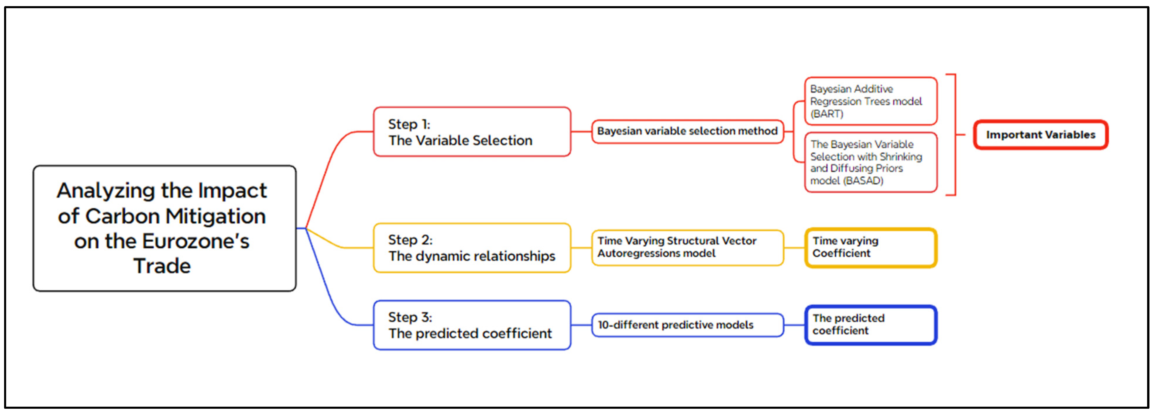
This study adopts a three-step methodological framework, variable selection, dynamic relationship modeling, and coefficient prediction, as presented in Figure 1. First, Bayesian variable selection methods (BART and BASAD) identify the key factors influencing trade under carbon mitigation policies. Next, the Time-Varying Structural Vector Autoregressions (TV-SVAR) model incorporates time-varying coefficients to capture evolving economic relationships and shifting trade dynamics. Finally, ten predictive models estimate the forecasted coefficient, ensuring a robust and reliable quantification of carbon mitigation’s future impact on trade.

In addition to identifying the dynamic effects of carbon mitigation policies on trade, this study extends its analysis to forecasting future impacts. Accurately predicting how key trade variables influence carbon emissions is critical for policymaking in a time of rapidly evolving environmental regulations. By estimating the future trajectories of time-varying coefficients, we provide a forward-looking perspective on how the carbon border adjustment mechanism (CBAM) may reshape trade relations. This predictive insight is particularly valuable for EU policymakers seeking to preemptively design adaptive trade measures and support industries likely to face environmental compliance challenges. It also equips trade partners—such as the US and China—with evidence to guide their production and export strategies in alignment with emerging EU sustainability benchmarks. In this way, forecasting becomes not only an analytical tool but also a strategic asset for achieving long-term climate and economic objectives.

2. Literature Reviews

This section reviews the relevant empirical and economic literature on carbon mitigation and trade. To ensure comprehensive coverage, we conducted a targeted search of the Web of Science and Scopus databases using keywords such as “CBAM,” “carbon leakage,” “trade emissions,” and including the “WTO.”

2.1. The Carbon Border Adjustment Mechanism (CBAM)

The carbon border adjustment mechanism (CBAM), introduced as a key element of the European Green Deal and institutionalized under the “Fit for 55” legislative package in 2021, represents a transformative policy tool designed to harmonize EU trade practices with its climate neutrality targets. Specifically, the CBAM addresses the issue of carbon leakage by imposing a carbon cost on selected imports based on their embedded emissions. This aims to ensure a level playing field between domestic EU industries subject to the emissions trading system (ETS) and foreign producers operating under less stringent environmental regulations (Lim et al., 2021).

Academic literature increasingly underscores the dual function of the CBAM as both a climate policy mechanism and a trade regulatory instrument. While studies such as Aichele and Felbermayr (2015) highlight its effectiveness in reducing global emissions and deterring carbon leakage, others caution against its potential conflict with international trade law. Lim et al. (2021), for example, warn that the CBAM could be perceived as a disguised restriction on international trade, conflicting with WTO principles of non-discrimination and national treatment. Furthermore, Eicke et al. (2021) emphasizes that the CBAM may disproportionately impact developing countries that lack the technological and institutional capacity to meet EU environmental standards, thereby raising concerns about equity and inclusiveness in global climate governance.

In addition to economic concerns, several studies have explored the legal implications of the CBAM. Bellora and Fontagné (2022) emphasize that ensuring WTO compliance requires careful design of the mechanism, particularly with respect to the principle of non-discrimination. They argue that, if the CBAM reflects domestic carbon pricing accurately and includes exemptions for least-developed countries, legal risks can be mitigated. Meanwhile, Deng and Guo (2024) highlight potential diplomatic tensions, especially with China and the United States, who may view the CBAM as a form of green protectionism. These countries have signaled the possibility of legal disputes to the WTO or reciprocal trade measures in response to the policy. These legal perspectives underscore the need to balance environmental ambition with trade diplomacy and multilateral obligations.

Previous empirical studies have examined the broader implications of carbon mitigation tools like the CBAM, particularly in relation to non-tariff measures and their role in shaping international trade flows (Monjon & Quirion, 2011). Branger and Quirion (2014) further argue that carbon pricing significantly alters trade dynamics in emissions-intensive sectors, yet there remains a gap in understanding the specific trade impacts between the EU and major partners such as the United States and China. To address this gap, recent econometric approaches have adopted Bayesian variable selection techniques, which are particularly effective in managing high-dimensional and multicollinear data—a common challenge in trade and environmental studies. Research by Narisetty and He (2014) and O’Hara and Sillanpää (2009) demonstrates that Bayesian methods not only enhance model robustness but also mitigate overfitting while retaining relevant predictors, making them especially suitable for analyzing complex policy interactions such as those presented by the CBAM.

2.2. The Econometric Models

2.2.1. Variable Selection (Bayesian Variable Selection Method)

The Bayesian variable selection techniques are essential tools for identifying relevant predictors in high-dimensional datasets, particularly when non-linearities and interactions may be present. In this study, we adopt two advanced Bayesian approaches: Bayesian Additive Regression Trees (BART) and Bayesian Shrinkage Additive Decomposition (BASAD). These models are especially suited to the complex structure of trade and environmental data, where relationships between variables are both dynamic and interdependent. Bayesian methods offer advantages over traditional frequentist approaches by incorporating prior beliefs and probabilistic inference. Unlike stepwise regression or lasso-based methods, which impose hard or penalized constraints, Bayesian variable selection allows for a more flexible and interpretable structure using priors. This is particularly valuable in sparse settings where only a few predictors may have meaningful influence.

Bayesian Additive Regression Trees, introduced by Chipman et al. (2010), is a non-parametric ensemble learning method that models the outcome as a sum over many small regression trees. Each tree captures a portion of the predictive structure, and regularization is achieved through priors that control the depth and impact of each tree. BART is particularly effective in detecting non-linear relationships and higher-order interactions without the need to specify them explicitly. BART’s ability to provide posterior inclusion probabilities makes it suitable for variable selection. Studies by Bleich et al. (2014) and Kapelner and Bleich (2016) developed formal permutation-based procedures and inferential methods to determine which predictors meaningfully contribute to the model. Moreover, the BART framework can incorporate prior information on variable importance, further enhancing its capacity to recover true underlying relationships in complex systems.

Meanwhile, Bayesian Shrinkage Additive Decomposition (BASAD), proposed by Ročková and George (2014), represents a scalable solution to Bayesian variable selection using spike-and-slab priors. It applies shrinkage directly to regression coefficients by decomposing the prior distribution into a “spike” near zero and a “slab” representing plausible non-zero values. This decomposition facilitates sparsity by strongly penalizing unimportant coefficients while retaining significant predictors. One major advantage of BASAD is its ability to retain the uncertainty quantification from the Bayesian framework while enabling scalable model selection. The method is especially effective in sparse high-dimensional contexts where the number of covariates far exceeds the sample size, a common feature in international trade data. By drawing from the posterior distribution over model configurations, BASAD ensures that selected predictors are not only statistically relevant but robust across plausible data-generating processes.

Together, BART and BASAD provide a complementary framework for Bayesian variable selection. BART excels at uncovering complex, non-linear interactions and variable importance, while BASAD offers rigorous shrinkage and sparsity control. Their combination improves both the predictive accuracy and interpretability of econometric models involving environmental and trade-related covariates. This dual approach enables the identification of structural linkages between carbon mitigation and international trade dynamics—laying the groundwork for the subsequent time-varying analysis using TV-SVAR.

2.2.2. The Time-Varying Structural Vector Autoregressions (TV-SVAR) Model

The Time-Varying Structural Vector Autoregressions (TV-SVAR) model is particularly valuable in analyzing economic relationships that evolve over time, making it more flexible than traditional models such as standard SVAR or fixed-coefficient models. TV-SVAR has the ability to capture structural changes and dynamic shifts in the relationships between variables, which is essential when studying the impact of policies like carbon mitigation in trade (Primiceri, 2005). Unlike fixed coefficient models that assume constant effects over time, TV-SVAR allows for time-varying coefficients, making it better suited for capturing the evolving nature of economic and environmental variables (Nakajima, 2011). Studies by Koop and Korobilis (2010) have shown that TV-SVAR is particularly effective in policy analysis, as it can account for changes in the economy or policy regimes, offering more accurate and adaptable results compared to models with static coefficients.

In short, Eicke et al. (2021) offers a critical perspective on the carbon border adjustment mechanism (CBAM), emphasizing the potential inequalities embedded in its design. The study contends that the CBAM may impose disproportionate burdens on developing economies, which often lack the technological capabilities and institutional frameworks necessary to comply with the EU’s stringent climate standards. This concern underscores broader questions about the distributive justice of global carbon policies and the feasibility of inclusive climate governance. However, while Eicke’s analysis is rich in normative critique, it remains largely qualitative and does not quantitatively explore how the CBAM affects trade composition of the EU. In response to this gap, our study extends the literature by employing a Bayesian econometrics framework that not only enhances variable selection under high-dimensional trade data but also allows for time-varying estimation of policy impacts. Furthermore, unlike previous research that aggregates trade at the sectoral level, we disaggregate EU imports by product categories and source countries, specifically, the United States and China, to offer a greater understanding of the CBAM’s differentiated impacts on future trade policy. Finally, we are able to capture both the direct environmental consequences and the broader trade-offs associated with implementing carbon mitigation tools in the context of global trade by using EU carbon emissions as the primary outcome variable.

3. Materials and Methods

3.1. Variable Selection (Bayesian Variable Selection Method)

This study employs Bayesian methods for variable selection which is a method used to identify the most relevant predictors in a model by using a probabilistic framework. This incorporates prior knowledge and updates it with observed data. Unlike traditional variable selection techniques, Bayesian methods account for model uncertainty and allow for model averaging, where the final model reflects the likelihood of various potential combinations of variables. This approach prevents overfitting and ensures the inclusion of only significant variables (George & McCulloch, 1993). In this study, two Bayesian techniques are employed: Bayesian Additive Regression Trees (BART) and Bayesian Shrinkage Additive Decomposition (BASAD).

3.1.1. Bayesian Additive Regression Trees (BART) Model

BART is a non-parametric approach that fits a sum-of-trees model. Each tree captures different aspects of the relationship between the independent variables and the dependent variable. BART is particularly useful when relationships between variables are complex and non-linear, and it automatically selects the most relevant variables based on their contribution to reducing prediction error (Chipman et al., 2010).

This model can be understood as an ensemble of decision trees, using a distinct estimation technique rooted in a fully Bayesian probability framework. Specifically, the model works by recursively partitioning the predictor space into hyperrectangles to approximate an unknown function ($f$). The dimension of the predictor space is determined by the number of variables, denoted as “$n$”.

$$Y=f\left(X\right)+\epsilon \approx T_1\left(X\right)+T_2\left(X\right)+\dots +T_m\left(X\right)+\epsilon ,\epsilon \sim {\mathcal{N}}_n\left(0,{\sigma }^2,I_n\right)$$

(1)

The BART framework expresses the response variable $Y$ as an additive function of multiple regression trees applied to the predictors $X$, combined with a stochastic error term “$\epsilon$” assumed to follow a normal distribution with zero mean and constant variance, $\epsilon \sim {\mathcal{N}}_n\left(0,{\sigma }^2{I}_n\right)$. Here, $X$ denotes the $n\times p$ design matrix, and each function $T_m\left(X\right)$ corresponds to the output of an individual regression tree within the ensemble. The assumption of independent and homoskedastic errors ensures the model remains tractable for posterior inference and variance decomposition.

Each tree in the ensemble contributes a unique component to the overall prediction, learning structure in the data by recursively partitioning the predictor space. By summing over these tree-based functions, BART is capable of modeling intricate non-linear relationships without requiring manual specification of interaction terms. The number of trees “$m$” plays a crucial role: a higher number of trees increases model expressiveness but can also introduce noise by fitting spurious patterns. Consistent with guidance from Chipman et al. (2010), we selected $m$ = 20, which offers a balance between predictive performance and effective variable selection.

The selection criteria use the 2nd quantile to set the split point, aiding in the sum-of-trees approach by identifying variables that significantly reduce prediction error. For the prior assumptions, we adopt the default priors as in Chipman et al. (2010), with a regularization prior on the tree depth.

3.1.2. The Bayesian Variable Selection with Shrinking and Diffusing Priors Model (BASAD)

The Bayesian Variable Selection with Shrinking and Diffusing Priors model was proposed by (Narisetty & He, 2014) to identify relevant covariates in a high-dimensional data settings. This approach is specifically designed to handle cases where the number of covariates ($p$) exceeds the number of observations ($n$), a common challenge in modern data analysis. We firstly consider the typical linear regression model where the response “$n\times 1$” is response vector “$Y$” and “$n\times p_n$” is design matrix “$X$” corresponding to the “$p_n$” covariates of interest. We have let “$\beta$” be the regression vector and it is sparse in the sense that only a few components are non-zero. The description of the model is as follows:

$$Y\left|\left(X,\beta ,{\sigma }^2\right)\sim N\left(X\beta ,{\sigma }^2,I\right),\right.$$

(2)

$${\beta }_i\left|\left({\sigma }^2,Z_i=0\right)\sim N\left(0,{\sigma }^2,{\tau }_{0,n}^2\right),\right.$$

(3)

$${\beta }_i\left|\left({\sigma }^2,Z_i=1\right)\sim N\left(0,{\sigma }^2,{\tau }_{1,n}^2\right),\right.$$

(4)

$$\mathrm{P}\left(Z_i=1\right)=1-\mathrm{P}\left(Z_i=0\right)=q_n,$$

(5)

$${\sigma }^2\sim IG\left({\alpha }_1,{\alpha }_2\right),$$

(6)

where “$i$” runs from 1 to “$p_n,q_n,{\tau }_{0,\mathrm{n}},{\tau }_{1,\mathrm{n}}$,” which are constants that depend on $n$. While the “$IG\left({\alpha }_1,{\alpha }_2\right)$” is the inverse gamma distribution with shape parameter “${\alpha }_1$” and scale parameter “${\alpha }_2$”.

This idea involves applying the shrinking and diffusing priors to improve the idea of spike-and-slab priors to facilitate variable selection. The shrinking and diffusing prior introduced in this model is designed to improve selection performance in high-dimensional settings by adapting the prior variances based on the covariate’s relevance: (1) shrinking: for covariates that are likely inactive, the variance “${\tau }_{0,n}^2$” is shrunk toward zero, which effectively minimizes the influence of irrelevant variables; (2) diffusing: for covariates that are likely active, the variance “${\tau }_{1,n}^2$” allows for greater flexibility, giving more weight to the covariates contributing significantly to the response.

Narisetty and He (2014) propose a Bayesian approach to select active covariates using shrinking and diffusing priors and the posterior probabilities “$\mathrm{P}\left(Z_i=1\left|Y,X\right.\right)$” for each covariate rather than searching the full model space. Covariates with marginal posterior probabilities above a chosen threshold (typically 0.5) are selected as active. This approach is referred to as the median probability model. The authors note that, while this model may differ from the maximum a posteriori (MAP) model, both converge to the same model with high probability under conditions of strong selection consistency. Finally, spike-and-slab priors were used with the spike variance ${\tau }_{0,n}^2$ set to 0.01 and slab variance ${\tau }_{1,n}^2$ set to 10. The prior inclusion probability for each variable was set to 0.5.

In summary, the BART and the BASAD models represent two different philosophies in Bayesian variable selection. The BART model excels in scenarios where the relationship between predictors and the outcome is complex and involves high-order interactions, albeit at the expense of interpretability. Meanwhile, the BASAD model provides a more structured and interpretable framework by modeling effects additively with smooth functions and employing shrinkage for variable selection, making it a strong candidate when the underlying relationships are expected to be largely additive and when interpretability is a priority.

3.2. Time-Varying Structural Vector Autoregressions Model

The Time-Varying Structural Vector Autoregressions (TV-SVAR) model allows for the dynamic relationships between multiple endogenous variables to change over time, making it particularly suitable for capturing evolving economic structures. The methodology involves specifying the observation and state equations, modeling the covariance structure, and using estimation techniques to infer the time-varying parameters (Primiceri, 2005). The basic form of the time-varying VAR model is

$$y_t=c_t+{\displaystyle \sum _{i=1}^p{y}_{t-i}{B}_i}+{\mu }_t;t=1,\dots ,\mathrm{T},$$

(7)

where the $y_t$ is a vector of endogenous variables (EU carbon emissions), $y_{t-i}$ is a vector containing the lags of the endogenous variables. The reduced form of the residual ($u_t$) can be decomposed as

$${\mu }_t=A_t^{-1}{\sum }_t{\epsilon }_t,{\epsilon }_t\sim N\left(0,1\right),$$

(8)

which is a time-varying matrix capturing the contemporaneous relationships among the variables. To achieve identification, this is often assumed to be lower triangular. ${\sum }_t$ is a diagonal matrix whose diagonal elements are the time-varying standard deviations of the shocks. Consequently, the variance–covariance matrix of $u_t$ is given by

$${\mathrm{\Omega }}_t={\mathrm{A}}_t^{-1}{\mathrm{\Sigma }}_t{\left(A_t^{-1}\right)}^{\prime },$$

(9)

3.2.1. Time Variation via State Equations

The state equations describe how the parameters of the model (the time-varying coefficients and elements of the impact matrix) evolve over time. We assume that the parameters follow random walk processes. Specifically, we let:

$$B_t=B_{t-1}+{\nu }_t;{\nu }_t\sim N\left(0,Q\right),$$

(10)

$${\alpha }_t={\alpha }_{t-1}+{\zeta }_t;{\zeta }_t\sim N\left(0,\mathrm{S}\right),$$

(11)

$$\log {\sigma }_t=\log {\sigma }_{t-1}+{\eta }_t;{\eta }_t\sim N\left(0,W\right),$$

(12)

where $B_t$ denotes the vectorized collection of the lag coefficients and ${\alpha }_t$ collects the free elements of $A_t$ (excluding those fixed by identification, such as the ones on the main diagonal). ${\sigma }_t$ are the diagonal elements of ${\mathrm{\Sigma }}_t$. The $Q,\mathrm{S}$, and $W$ are hyperparameter matrices governing the extent of time variation.

These state equations enable the model to reflect both slow-moving changes in the economic relationships and shifts in the magnitude of shocks. Given the high dimensionality and the non-linearities inherent in the TV-SVAR, we adopt a Bayesian approach and implement a Gibbs sampler to draw from the joint posterior distribution of the time-varying parameters and hyperparameters.

3.2.2. Identification and Structural Interpretation

The structural interpretation of shocks is achieved by imposing restrictions on the $A_t$ matrix. A common strategy is to assume a lower triangular form for $A_t$, which effectively orthogonalizes the shocks. This identification is critical, as it ensures that the estimated structural shock obtained via the relation.

$${\epsilon }_t={\mathrm{\Sigma }}_t^{-1}{\mathrm{A}}_t{\mu }_t$$

(13)

This can be interpreted in economically meaningful ways. With the time-varying setup, the model permits both the size of the shocks (captured by ${\mathrm{\Sigma }}_t$) and the instantaneous interactions among variables (captured by $A_t$) to change over time.

Finally, this methodology offers a flexible approach to analyzing how macroeconomic and trade dynamics evolve over time. By allowing both the coefficients and the variance structure to vary, the model captures whether changes in outcomes are driven by shifts in transmission channels or by changes in the size of external shocks. The model was estimated using the tvReg package in R (version 4.2.1), which applies local constant kernel smoothing to generate time-varying parameter estimates. Since this approach does not rely on iterative sampling, standard convergence diagnostics such as R-hat values or trace plots are not applicable. Instead, the bandwidth for smoothing was selected using cross-validation to ensure that the estimates remained stable and reliable throughout the sample period.

To identify contemporaneous structural relationships, we employed a recursive identification strategy using the Cholesky decomposition of the residual covariance matrix at each time point. The ordering of variables was based on economic reasoning: control variables (GDPs and exchange rates) were placed first, followed by trade variables, and carbon emissions were ordered last. This structure reflects the assumption that emissions respond to trade and macroeconomic shocks within the same month but do not influence them contemporaneously. This approach is widely used in Time-Varying SVAR studies and was tested for robustness using alternative orderings, which produced similar qualitative results.

3.3. Software and Reproducibility

All computations were conducted using R (version 4.2.1). The following packages were employed: “bartMachine” for Bayesian Additive Regression Trees (BART), “BASAD” for Bayesian variable selection with shrinkage priors, “tvReg” for estimating the Time-Varying Structural Vector Autoregressions (TV-SVAR) model, and “forecast” for generating predictive projections.

3.4. Data

The dataset used in this study comprises monthly observations covering the period from May 2011 through September 2023, resulting in a total of 149 records. The data were compiled from multiple sources, including Eurostat, the European Central Bank, and the CEIC database, ensuring consistency and credibility for empirical analysis of carbon emissions in the European Union (EU). For a comprehensive examination, the study’s variables are categorized into three distinct groups, encompassing a total of 53 variables.

(1)

The main outcome variable in this analysis is the total volume of carbon emissions reported within the European Union (EU). It is used as the key metric for evaluating how the proposed policy tools may influence environmental performance.

(2)

The explanatory variables consist of 15 major categories of EU import goods, reflecting the trade patterns of the EU with China and the USA, as shown in the following table. This is the total value of each imported goods category to the EU, expressed in euros. Totally, the independent variables are 30 EU import goods (

Table 1. The list of independent variables.

	Description		Description		Description
x1	Food, Drink and Tobacco	x6	Mineral Fuels and Lubricants	x11	Other Manufactured Products
x2	Live Animals	x7	Petroleum Products	x12	Manufactured Gds
x3	Beverages and Tobacco	x8	Animals and Vegetable Oils	x13	Machinery and Transport Equip
x4	Raw Materials	x9	Manufactured Products	x14	Miscellaneous Mfg. Articles
x5	Crude Materials Inedible	x10	Chemicals and Related Pdts	x15	Goods nes

).

(3)

The control variables were selected to account for external factors influencing EU international trade. This group comprises two key groups of variables: 1. GDP levels from major economies, including the EU, the US, and China; 2. exchange rates relative to the EU currency, specifically the US dollar/euro, and yuan/euro. The inclusion of these control variables is essential for distinguishing the effects of the main explanatory variables, thereby improving the precision and robustness of the results. In total, the model incorporates five control variables.

A summary of the variables reveals that most series display positive central tendencies based on their mean, median, and range (maximum and minimum) values. The Jarque–Bera (JB) normality test suggests that the distributions of these variables are generally non-normal, a finding supported by skewness and kurtosis statistics. This confirms that the data deviate from the normality assumption commonly used in parametric analysis.

4. Results

4.1. Variable Selection

The variable selection is crucial due to the presence of 52 potential explanatory variables for EU carbon emissions, which makes it necessary to identify the most relevant ones to avoid overfitting and improve model interpretability. To address this, we employ two Bayesian variable selection methods, specifically the Bayesian Additive Regression Trees (BART) and Bayesian Shrinkage Additive Decomposition (BASAD) models by integrating their results for variable selection which offers a balanced strategy that leverages the strengths of both methods. Ultimately, this integrated approach balances predictive complexity with parsimony, yielding models that are not only accurate but also interpretable and thus more reliable for informed decision making.

(1)

For the BART model, we set the split point ($c$) at the quantile criterion at the 2nd quantile which helps in determining the splitting rules within the sum-of-trees approach, focusing on identifying variables that significantly contribute to reducing prediction error.

(2)

For the BASAD model, covariates were selected based on their marginal posterior probabilities, with a chosen threshold of 0.5, indicating that only variables with a probability above this threshold are retained as significant predictors. By cross-referencing the results from both methods, we were able to identify the key variables that consistently emerged as significant across both approaches, ensuring a more robust and comprehensive selection of predictors for the subsequent analysis.

After applying the Bayesian variable selection methods, the integrated results from BART and BASAD models highlighted three key variables that consistently emerged as significant (

Table 2. Variable Selection.

BART Model	BASAD Model
US_x13	Yuan/Euro	CH_x8
US_x12	US_x9	CH_x3
CH_x12	US_x12	CH_x2
CH_x6	TH_x8	US_x8
US_x15	US_x3
US_x2	CH_x4
US_x10	CH_x7
US_x11	US_x7
US_x9	CH_x1
CH_x7	CH_x15
Integrated (BART model and BASAD model)
Variable		Name
US_x9		Manufactured Products from the US
US_x12		Manufactured Goods from the US
CH_x7		Petroleum Products from China

Note: Chosen thresholds are 0.5.

): US_x9 (manufactured products from the US), US_x12 (manufactured goods from the US), and CH_x7 (petroleum products from China). These variables indicate the importance of manufactured and petroleum products in understanding the effects of carbon mitigation policies on trade patterns between the EU and its major trade partners, specifically, the United States and China. The prominence of these variables suggests that shifts in the trade of these product categories may have a substantial impact on the carbon footprint and trade dynamics of the Eurozone.

4.2. The Model Selection

We begin by selecting the most appropriate panel regression model for our dataset through comparative analysis. This method is based on the understanding that different economic phenomena can exhibit diverse behaviors and relationships within the data. To identify the most suitable estimation model, we use the Akaike information criterion (AIC) and Bayesian information criterion (BIC) as selection criteria.

This makes it necessary to identify the most relevant variables to avoid overfitting and improve model interpretability. To address this, we employ two Bayesian variable selection methods, specifically the Bayesian Additive Regression Trees (BART) and Bayesian Shrinkage Additive Decomposition (BASAD) models, by integrating their result for variable selection which offers a balanced strategy that leverages the strengths of both methods. Ultimately, this integrated approach balances predictive complexity with parsimony, yielding models that are not only accurate but also interpretable and thus more reliable for informed decision making.

Our analysis compares the Time-Varying Structural Vector Autoregressions (TV-SVAR) model and the State Space model, alongside static regression methods like Ordinary Least Squares (OLS) Regression and Lasso Regression. This comparison aims to determine whether our proposed model offers a better fit than traditional models.

Table 3. Model Selection.

		AIC	BIC
Static model	OLS Regression model	−5.802	−4.899
	Lasso Regression model	−12.323	−12.001
Dynamic model	State Space model	−19.226	−18.324
	Time-Varying Structural Vector Autoregressions	−22.241	−22.117

presents the AIC and BIC values used for model selection, indicating that the Time-Varying Structural Vector Autoregressions (TV-SVAR) model outperforms both dynamic and static regression models, as reflected in its lower AIC and BIC scores. These results suggest that the TV-SVAR model provides a greater understanding of the data compared to the alternative models.

4.3. The Estimated Result

The Time-Varying Structural Vector Autoregressions (TV-SVAR) model allows us to examine how the impact of these selected predictors on EU carbon emissions evolves over time. The TV-SVAR model is particularly well-suited for this analysis, as it captures the dynamic nature of economic relationships, revealing how changes in trade patterns and policies affect carbon emissions across different time periods. By utilizing this model, we can gain insights into the fluctuating effects of each predictor on the EU’s carbon footprint, thereby providing a clearer understanding of the interplay between trade dynamics and environmental outcomes.

We present the dynamic patterns of how EU import goods influence carbon emissions within the EU, as revealed through the Time-Varying Structural Vector Autoregressions (TV-SVAR) model, in

Table 4. Time-Varying Structural Vector Autoregressions model result.

	Intercept	US_x9	US_x12	CH_x7
		Manufactured Products from the US	Manufactured Goods from the US	Petroleum Products from China
Min.	161.800	−0.006	−3.460	2.261
Median	238.300	0.005	−1.864	3.783
Mean	245.700	0.004	−1.863	3.727
Max.	389.700	0.009	−0.034	4.948

and Figure 2. This model enables us to trace how the effects of key variables shift over time, and these patterns are visualized in the accompanying figures. Through this approach, we highlight how the strength and direction of each variable’s influence fluctuate across the sample period, offering a more detailed view of their dynamic behavior. This temporal resolution is especially helpful in pinpointing intervals during which certain variables exert stronger or weaker effects.

Firstly, the estimated coefficients for manufactured products from the US (US_x9) range from −0.006 to 0.009, with a mean of 0.004, indicating a small but positive time-varying effect on EU carbon emissions. This suggests that increased imports of these products slightly raise carbon emissions, likely due to the carbon-intensive nature of US manufacturing processes and the emissions associated with transportation logistics (Hertwich & Peters, 2009; Mayor & Tol, 2008). However, the graph reveals a gradual downtrend in this impact over time, suggesting that the carbon footprint of these imports has diminished as production methods in the US become more energy-efficient and aligned with cleaner technologies. This trend presents an opportunity for the EU to promote imports of lower-carbon goods through targeted trade agreements, aligning with its carbon reduction goals while maintaining strong trade relations with the US.

Manufactured goods (US_x12) from the US range from −3.460 to −0.034, with a mean of −1.863, indicating that increased imports of these goods tend to reduce EU carbon emissions over time. This negative relationship suggests that the shift in production to the US, where stricter emission standards and more energy-efficient practices prevail, has allowed the EU to benefit from reduced local emissions while still accessing necessary goods (Sauvage, 2014). However, the trend shows a notable uptrend over time, meaning that the negative impact of these imports on emissions has lessened, with the coefficients becoming closer to zero. This change implies that the initial environmental benefits of shifting production are diminishing, potentially due to changes in production practices or increased import volumes.

Finally, petroleum products from China (CH_x7) range from 2.261 to 4.948, with a mean value of 3.727, indicating a strong positive relationship between these imports and EU carbon emissions. This suggests that increased imports of petroleum products from China correlate with reduced carbon emissions in the EU, likely due to a substitution effect where the EU decreases its carbon-intensive domestic petroleum production and relies more on imports (Khan et al., 2020). This trend aligns with the EU’s growing emphasis on renewable energy, which has lessened the need for locally produced fossil fuels. However, the graph reveals a slight upward trend, indicating that the initial negative impact of these imports on EU emissions is diminishing over time. This change may reflect shifts in the global energy market or the EU’s continued investment in renewables, which reduces the comparative benefits of imported petroleum.

The TV-SVAR analysis sheds light on the evolving effects of different imports on EU carbon emissions. Manufactured products from the US (US_x9) display a slight positive effect, reflecting the ongoing carbon intensity of US-manufactured products. US_x12 shows a negative effect, suggesting that importing these goods may reduce emissions through shifts in production. Meanwhile, petroleum products from China (CH_x7) demonstrate a significant positive impact. Together, these insights emphasize the complex interactions between trade dynamics and carbon emissions, highlighting the importance of trade patterns in shaping the Eurozone’s environmental outcomes.

4.4. The Predicted Coefficient Result

This step of the analysis is to predict the time-varying coefficients obtained from the Time-Varying Structural Vector Autoregressions (TV-SVAR) model to provide a future perspective on how key trade variables will impact EU carbon emissions. This future view is essential for policymakers, as it can inform decisions on trade and environmental policies by highlighting anticipated changes in the carbon impact of imports over time.

To accomplish this, the predictive models were trained and evaluated using the full in-sample dataset consisting of 149 monthly observations from May 2011 to September 2023. A total of ten forecasting models were tested to identify the most suitable one for predicting the time-varying effects of trade on EU carbon emissions. Although out-of-sample validation was not conducted, model robustness was assessed through comparative performance across multiple algorithms. The evaluation was based on two key metrics: mean absolute percentage error (MAPE) and mean absolute deviation (MAD), both of which measure the accuracy and precision of the predictions. Lower values of MAPE and MAD indicate better model performance in terms of minimizing error and deviation from actual data (

Table 5. Selection of prediction model.

	Manufactured Products from the US		Manufactured Goods from the US		Petroleum Products from China
	MAPE	MAD	MAPE	MAD	MAPE	MAD
1. Arimaa	1.2 × 10−5	5.8 × 10−8	1.2 × 10−5	3.3 × 10−5	1.2 × 10−5	3.3 × 10−5
2. BaggedModela	9.0 × 10−5	4.7 × 10−7	2.1 × 10−4	7.4 × 10−4	2.1 × 10−4	7.4 × 10−4
3. Etsa	1.6 × 10−3	8.4 × 10−6	1.2 × 10−5	4.0 × 10−5	1.2 × 10−5	4.0 × 10−5
4. BaggedModel_arimaa	8.3 × 10−5	4.3 × 10−7	1.8 × 10−4	6.4 × 10−4	1.8 × 10−4	6.4 × 10−4
5. Nnetara	5.5 × 10−5	2.9 × 10−7	1.4 × 10−4	5.3 × 10−4	1.4 × 10−4	5.3 × 10−4
6. Meanfa	5.3 × 10−2	2.8 × 10−4	1.2 × 10−1	4.6 × 10−1	1.2 × 10−1	4.6 × 10−1
7. Rwfa	1.5 × 10−3	8.0 × 10−6	3.6 × 10−3	1.3 × 10−2	3.6 × 10−3	1.3 × 10−2
8. Thetafa	1.5 × 10−3	8.0 × 10−6	3.6 × 10−3	1.3 × 10−2	3.6 × 10−3	1.3 × 10−2
9. Holta	3.3 × 10−5	1.7 × 10−7	1.2 × 10−5	4.0 × 10−5	1.2 × 10−5	4.0 × 10−5
10. Splinefa	1.4 × 10−4	6.7 × 10−7	1.2 × 10−4	3.5 × 10−4	1.2 × 10−4	3.5 × 10−4

). Among the models tested, the Arima model was identified as the most suitable predictive model, as it had the lowest MAPE and MAD values across all key variables: manufactured products from the US, manufactured goods from the US, and petroleum products from China. This model will be used for further prediction analysis, providing a robust framework for understanding future carbon emissions impacts from trade with these countries.

The results of the predicted time-varying coefficients over the next 24 months provide critical insights into the future impact of key imports on EU carbon emissions (Figure 3). The predicted time-varying coefficients for manufactured products from the US (US_x9) indicate a decreasing impact on EU carbon emissions (Figure 3a). This trend suggests that these products may have a reduced carbon footprint in the future, potentially exempting them from stricter environmental regulations. In contrast, the forecast for manufactured goods from the US (US_x12) reveals an upward trend (Figure 3b), indicating that these imports will contribute more significantly to EU carbon emissions over time, necessitating stronger regulatory measures to mitigate their environmental impact. US policymakers should encourage cleaner, energy-efficient production for manufactured goods (US_x12) to reduce their growing carbon footprint and avoid stricter EU trade regulations. Meanwhile, the decreasing impact of manufactured products (US_x9) presents an opportunity to further promote sustainable manufacturing, strengthening trade ties with the EU and supporting global climate goals.

Similarly, petroleum products from China (CH_x7) show a projected increase in their contribution to EU carbon emissions, highlighting the need for more aggressive environmental policies (Figure 3c). As the carbon intensity of these imports rises, policymakers will need to consider implementing stricter trade barriers or carbon pricing mechanisms to align these imports with the EU’s sustainability goals. Chinese policymakers should focus on reducing the carbon intensity of petroleum products (CH_x7), which are projected to increase EU carbon emissions. By promoting cleaner energy sources and improving production efficiency, China can mitigate the risk of facing stricter EU trade barriers or carbon pricing. Implementing such measures will not only help maintain access to EU markets but also support global efforts to reduce carbon emissions.

5. Discussion and Limitations

5.1. The Discussion

The findings of this study reveal significant implications for international trade dynamics in the context of carbon mitigation, particularly for the Eurozone and its major trading partners—the US and China. The analysis highlights the evolving relationship between carbon emissions and trade, underscoring the need for adaptive policy responses to align with global environmental objectives. The results suggest that manufactured products from the US currently have a small but positive time-varying effect on the Eurozone’s carbon emissions. However, the observed downward trend over time indicates a decline in their environmental impact. This finding reflects potential improvements in production efficiency or stricter environmental regulations being adopted by US manufacturers. From a policy perspective, this trend is encouraging, as it suggests that certain US-manufactured goods could eventually contribute to reducing the EU’s carbon footprint. As these products continue to exhibit diminishing emissions effects, they may become less susceptible to future non-tariff environmental barriers within the EU, potentially maintaining their competitive advantage in European markets.

In contrast, the analysis reveals a concerning trend for manufactured goods from the US and petroleum products from China, both of which exhibit a positive trajectory in their contribution to the EU’s carbon emissions. This suggests a growing environmental impact over time, likely due to increasing trade volumes, reliance on carbon-intensive production processes, or insufficient implementation of cleaner technologies. As the EU continues to strengthen its commitment to climate change mitigation, these goods could become prime targets for stricter measures, such as carbon tariffs or import restrictions. Such actions would align with the EU’s broader carbon mitigation strategies and its goal of incentivizing cleaner production practices among its trading partners.

Overall, these findings emphasize the importance of adaptive and forward-looking trade policies in response to evolving environmental challenges. The EU’s potential implementation of non-tariff measures on high-carbon imports highlights the growing intersection between trade and environmental governance. For trading partners like the US and China, aligning production processes with global environmental standards will not only help mitigate climate change but also ensure continued access to the increasingly environmentally conscious European market. Additionally, the study’s implications are aligned with broader Sustainable Development Goals (SDGs). This study contributes to supporting SDG 13 (Climate Action) by highlighting the importance of carbon-conscious trade and SDG 17 (Partnerships for the Goals) by underscoring the need for cooperative trade and climate strategies between advanced and developing economies and to a deeper understanding of how carbon mitigation policies influence international trade flows and underscores the importance of integrating sustainability considerations into future trade strategies.

5.2. Limitations and Future Directions

This study provides important insights into the relationship between carbon mitigation and trade, while several limitations should be acknowledged. First, there remains the possibility of omitted variable bias or reverse causality, particularly where carbon emissions may indirectly influence trade patterns or policy responses. Although the Bayesian variable selection method reduces this risk, the presence of unobserved feedback mechanisms cannot be entirely ruled out. In addition, the use of monthly data and the dynamic changes may not fully reflect long-term or lagged environmental effects, especially in industries with slower adjustment cycles. Second, the classification of imports into broad product categories such as “manufactured goods” and “petroleum products” may mask underlying variations in carbon intensity across sub-sectors.

Future research could benefit from more detailed trade data or firm-level carbon emission profiles to increase accuracy. It is also recommended that future studies expand the analysis to include exports and bilateral trade flows. Furthermore, developing countries beyond China and the US—such as those in Southeast Asia, Africa, or Latin America—should be considered, as they may face higher adjustment costs under the CBAM framework. These extensions would help improve the policy relevance of the findings and align with global sustainability goals, particularly SDG 13 (Climate Action) and SDG 17 (Partnerships for the Goals).

6. Conclusions

This study has provided a comparative assessment of the effectiveness of carbon mitigation strategies, particularly carbon pricing mechanisms for international trade, in influencing trade dynamics between the Eurozone and key trading partners, namely, the USA and China. The research employed advanced Bayesian variable selection methods and a Time-Varying Structural Vector Autoregressions (TV-SVAR) model to identify and analyze the variables most significantly affecting carbon emissions within this trade context. This methodological approach allowed us to capture the evolving impact of trade-related imports on EU carbon emissions, shedding light on how these effects vary over time and differ between trade partners.

The findings provide critical insights for EU policymakers and trade partners. Manufactured products from the US (US_x9) currently have a minor positive impact on EU carbon emissions, but this effect is decreasing over time, suggesting they may be exempt from future environmental regulations. Conversely, manufactured goods from the US (US_x12) and petroleum products from China (CH_x7) are expected to contribute more to EU emissions over time, indicating the need for stricter trade regulations.

References

1. Aichele, R., & Felbermayr, G. (2015). Kyoto and carbon leakage: An empirical analysis of the carbon content of bilateral trade. Review of Economics and Statistics, 97(1), 104–115. [Google Scholar] [CrossRef]
2. Bellora, C., & Fontagné, L. (2022). EU carbon border adjustment mechanism: A trade-relations perspective. CEPII working paper No. 2022-01. Available online: https://cepii.fr/PDF_PUB/wp/2022/wp2022-01.pdf (accessed on 23 June 2025).
3. Bleich, J., Kapelner, A., George, E. I., & Jensen, S. T. (2014). Variable selection for BART: An application to gene regulation. The Annals of Applied Statistics, 8(3), 1750–1781. [Google Scholar] [CrossRef]
4. Branger, F., & Quirion, P. (2014). Would border carbon adjustments prevent carbon leakage and heavy industry competitiveness losses? Insights from a meta-analysis of recent economic studies. Ecological Economics, 99, 29–39. [Google Scholar] [CrossRef]
5. Chipman, H. A., George, E. I., & McCulloch, R. E. (2010). BART: Bayesian additive regression trees. arXiv, arXiv:0806.3286. [Google Scholar] [CrossRef]
6. Clora, F., Yu, W., & Corong, E. (2023). Alternative carbon border adjustment mechanisms in the European Union and international responses: Aggregate and within-coalition results. Energy Policy, 174, 113454. [Google Scholar] [CrossRef]
7. Deng, H., & Guo, Y. (2024). Unveiling Carbon Border Adjustment Mechanism (CBAM): Challenges & potential dispute between China and EU. CORE Repository. Available online: https://core.ac.uk/download/pdf/548629074.pdf (accessed on 23 June 2025).
8. Eicke, L., Weko, S., Apergi, M., & Marian, A. (2021). Pulling up the carbon ladder? Decarbonization, dependence, and third-country risks from the European carbon border adjustment mechanism. Energy Research & Social Science, 80, 102240. [Google Scholar] [CrossRef]
9. European Commission. (2021). Data on the EU’s trade deficit with China. European Commission. [Google Scholar]
10. European Commission. (2023). Carbon Border Adjustment Mechanism (CBAM). Available online: https://ec.europa.eu (accessed on 1 December 2024).
11. George, E. I., & McCulloch, R. E. (1993). Variable selection via Gibbs sampling. Journal of the American Statistical Association, 88(423), 881–889. [Google Scholar] [CrossRef]
12. Hertwich, E. G., & Peters, G. P. (2009). Carbon footprint of nations: A global, trade-linked analysis. Environmental Science & Technology, 43(16), 6414–6420. [Google Scholar] [CrossRef] [PubMed]
13. International Energy Agency (IEA). (2021). World energy outlook 2021. International Energy Agency. Available online: https://www.iea.org (accessed on 1 December 2024).
14. Kapelner, A., & Bleich, J. (2016). bartMachine: Machine learning with Bayesian additive regression trees. Journal of Statistical Software, 70(4), 1–40. [Google Scholar] [CrossRef]
15. Khan, Z., Ali, M., Jinyu, L., Shahbaz, M., & Siqun, Y. (2020). Consumption-based carbon emissions and trade nexus: Evidence from nine oil exporting countries. Energy Economics, 89, 104806. [Google Scholar] [CrossRef]
16. Koop, G., & Korobilis, D. (2010). Bayesian multivariate time series methods for empirical macroeconomics. Foundations and Trends® in Econometrics, 3(4), 267–358. [Google Scholar] [CrossRef]
17. Lim, B., Hong, K., Yoon, J., Chang, J. I., & Cheong, I. (2021). Pitfalls of the EU’s carbon border adjustment mechanism. Energies, 14(21), 7303. [Google Scholar] [CrossRef]
18. Mayor, K., & Tol, R. S. (2008). The impact of the EU–US Open Skies agreement on international travel and carbon dioxide emissions. Journal of Air Transport Management, 14(1), 1–7. [Google Scholar] [CrossRef]
19. Monjon, S., & Quirion, P. (2011). Addressing leakage in the EU ETS: Border adjustment or output-based allocation? Ecological Economics, 70(11), 1957–1971. [Google Scholar] [CrossRef]
20. Nakajima, J. (2011). Time-varying parameter VAR model with stochastic volatility: An overview of methodology and empirical applications. Monetary and Economic Studies, 29, 107–142. [Google Scholar]
21. Narisetty, N. N., & He, X. (2014). Bayesian variable selection with shrinking and diffusing priors. Annals of Statistics, 42(2), 789–817. [Google Scholar] [CrossRef]
22. O’Hara, R. B., & Sillanpää, M. J. (2009). A review of Bayesian variable selection methods: What, how and which. Bayesian Analysis, 4(1), 85–117. [Google Scholar] [CrossRef]
23. Primiceri, G. E. (2005). Time varying structural vector autoregressions and monetary policy. The Review of Economic Studies, 72(3), 821–852. [Google Scholar] [CrossRef]
24. Ročková, V., & George, E. I. (2014). EMVS: The EM approach to Bayesian variable selection. Journal of the American Statistical Association, 109(506), 828–846. [Google Scholar] [CrossRef]
25. Sauvage, J. (2014). The stringency of environmental regulations and trade in environmental goods. OECD. [Google Scholar]
Figure 1. The conceptual framework.
Econometrics 13 00028 g001
Figure 2. The Time-Varying coefficients ( β t ) of (a) the Manufactured Products from the US; (b) Manufactured Goods from the US; (c) Petroleum Products from China covering the study period. The black solid line represents the posterior mean of the time-varying coefficient estimate at each time point. The grey shaded area denotes the credible interval (typically 68% or 95%) around the mean, reflecting the uncertainty in the coefficient estimates at each month. The red dashed vertical line marks a notable structural change point or policy intervention.
Econometrics 13 00028 g002
Figure 3. The predicted Time-Varying coefficients ( β t ) of (a) the Manufactured Products from the US; (b) Manufactured Goods from the US; (c) Petroleum Products from China. This shows forecasted marginal effects over a 24-month period.
Econometrics 13 00028 g003