
The Effect of Macroeconomic Announcements on U.S. Treasury Markets: An Autometric General-to-Specific Analysis of the Greenspan Era


Abstract
1. Introduction
2. Review of the Literature
2.1. Treasury Markets
2.2. Equity Markets
2.3. Gets in Finance and Elsewhere
3. Econometric Methodology
3.1. Equation (1)—Standard Static Regression Model (SSR)
3.2. Equation (2)—The General-to-Specific (Gets) Framework
- AR 1-2 test is a Lagrange multiplier test for rth-order autocorrelation, based on (Godfrey, 1978);
- ARCH test is based on (Engle, 1982);
- Normality Test—Chi2 form of (Doornik & Hansen, 2008);
- Hetero test for heteroscedastic errors based on (White, 1980);
- Regression Specification Error Test (RESET) based on (Ramsey, 1969).
- 6.
- Chow Predictive Failure Test based on (Chow, 1960);
- 7.
- Encompassing Tests between competing terminal models as in (Sargan, 1959; Govaerts et al., 1994).
3.3. Indicator Saturation Techniques
3.4. Comparing Models
4. Data
- 8.
- MMS Macroeconomic Announcement Dataset: This dataset includes detailed macroeconomic announcement data, capturing release timings, expectations, and as-reported actual values for key economic indicators.13
- 9.
- CRSP U.S. Treasuries Database: Provides daily U.S. Treasury returns and facilitates the calculation of excess returns as the difference between observed returns and the risk-free rate. This study uses daily returns data for U.S. Treasury securities.
4.1. Macroeconomic Announcement Data
- Employment reports (e.g., NonFarm Payrolls);
- Inflation measures (e.g., CPI, PPI);
- GDP growth;
- Consumer confidence and housing indices.
4.2. Treasury Return Data
5. Empirical Results
5.1. Selected Models
5.2. Diagnostic Tests
5.3. Model and Parameter Stability
5.4. Efficient Markets—Momentum and Mean Reversion
5.5. Corrections for Model Selection Bias
5.6. Encompassing Tests
6. Remarks
- Nonfarm Payrolls Shock (Scenario 1): The Gets model estimates a smaller negative price impact (−0.95 vs. −1.17 for SSR), leading to a $10,599 lower estimated trading loss for a typical transaction.
- Hourly Earnings Shock (Scenario 2): Again, the SSR model exhibits excessive sensitivity (−0.75 vs. −0.20 in Gets), resulting in a $26,800 larger estimated loss than the Gets model.
- Simultaneous Shocks to both Nonfarm Payrolls and Hourly Earnings (Scenario 3): The compounded impact is significantly smaller under Gets (−1.26 vs. −1.90 in SSR), translating to $31,173 less trading loss.
- Employment Cost Index (ECI) Shock (Scenario 4): Interestingly, the Gets model estimates a larger impact (−2.36 vs. −0.93 in SSR), suggesting that ECI shocks drive a more pronounced repricing under Gets. This results in an estimated $69,073 greater trading loss if Gets is more accurate, implying that traditional SSR models may have underestimated the market’s reaction to labor cost shocks.
7. Conclusions
Supplementary Materials
Funding
Data Availability Statement
Acknowledgments
Conflicts of Interest
Appendix A
Appendix A.1. US Treasury Yields and Term Spread

Appendix A.2. Rational Expectations of Macro Announcements Literature

| A. Rational Expectations | B. Anchoring Bias | |||
|---|---|---|---|---|
| Aggarwal et al. (1995) | Schirm (2003) | S. D. Campbell and Sharpe (2009) | Hess & Orbe (2013) | |
| Auto Sales | ||||
| Business Inventories | X | |||
| Capacity Utilization | X | |||
| Consumer Confidence | X | X | ||
| Construction Spending | X | |||
| CPI | ✓ | ✓ | Mixed case | X |
| Core CPI | Mixed case | X | ||
| Durable Goods Orders | X | X | X | X |
| Employment Cost Index | ||||
| Gross Domestic Product | ||||
| GDP Price Deflator | ||||
| Trade Balance | ✓ | ✓ | ✓ | |
| Hourly Earnings | X | |||
| Home Sales | ✓ | |||
| Housing Starts | ✓ | ✓ | X | |
| Industrial Production | X | X | X | X |
| Index of Lead. Econ. Ind. | X | X | ||
| ISM Manufacturing (NAPM) | ✓ | X | ||
| Nonfarm Payrolls | ✓ | ✓ | ✓ | |
| Personal Cons. Expenditures | X | |||
| Personal Income | ✓ | Mixed case | ✓ | |
| PPI | X | X | X | |
| Core PPI (ex: food and energy) | X | |||
| Retail Sales | X | ✓ | X | X |
| Retail Sales (ex: Auto Sales) | X | X | ||
| Unemployment Rate | ✓ | ✓ | ✓ | |
| Sample Start | Varies | 05/1990 | Varies | Varies |
| Sample End | 1993 | 12/2000 | 03/2006 | 2009 |
| Method | DF and ADF, Engle-Yoo | ADF, Engle-Yoo | AR(5), anchoring bias and Wald tests | ARIMA models, anchoring bias tests |
| Survey | MMS | MMS and TF | MMS | MMS |
| Key: | ✓ = RE | ✓ = RE | ✓ = no anchoring bias | ✓ = no anchoring bias |
| X = no RE | X = no RE | X = anchoring bias | X = anchoring bias | |
Appendix A.3. 10-Year Note Estimation Results
| 10-Year On-the-Run | 10-Year 1st Off-the-Run | ||||
|---|---|---|---|---|---|
| Indicators | Abbreviation | SSR | GETS | SSR | GETS |
| Coefficient | Coefficient | Coefficient | Coefficient | ||
| Constant | C | 0.097 ** | 0.107 ** | ||
| Auto Sales | SS_AUTOS | −0.144 | −0.150 | ||
| Business Inventories | SS_BUSINV | 0.013 | 0.021 | ||
| Capacity Utilization | SS_CAPACIT | −0.383 * | −0.391 * | ||
| Consumer Confidence | SS_CONFIDN | −0.651 ** | −0.629 ** | −0.628 ** | −0.689 ** |
| Construction Spending | SS_CONSTRC | −0.039 | −0.032 | ||
| Consumer Price Index | SS_CPI | −0.135 | −0.153 | ||
| Core CPI (ex: food and energy) | SS_CPIXFE | −0.428 ** | −0.567 ** | −0.394 ** | −0.581 ** |
| Durable Goods Orders | SS_DURGDS | −0.421 ** | −0.393 ** | −0.410 ** | −0.420 ** |
| Employment Cost Index | SS_ECI | −0.779 ** | −0.730 ** | −1.150 ** | |
| Gross Domestic Product | SS_GDP | −0.139 | −0.094 | ||
| GDP Price Deflator | SS_GDPPRIC | −0.197 | −0.215 | ||
| Goods and Services | SS_GDSSERV | 0.033 | 0.040 | ||
| Hourly Earnings | SS_HREARN | −0.578 ** | −0.630 ** | −0.557 ** | −0.405 ** |
| Home Sales | SS_HSLS | −0.524 ** | −0.487 ** | −0.549 ** | −0.608 ** |
| Housing Starts | SS_HSTARTS | −0.045 | −0.052 | ||
| Industrial Production | SS_INDPROD | 0.058 | 0.082 | ||
| Index of Lead. Econ. Ind. | SS_LEI | −0.070 | −0.071 | ||
| Nat. Assoc. of Purch. Mgrs. | SS_NAPM | −0.824 ** | −0.883 ** | −0.767 ** | −0.774 ** |
| Nonfarm Payrolls | SS_NONFARM | −1.070 ** | −0.769 ** | −1.030 ** | −0.797 ** |
| Personal Cons. Expenditures | SS_PCE | −0.058 | −0.052 | ||
| Personal Income | SS_PERSINC | −0.175 | −0.189 | ||
| Producer Price Index | SS_PPI | 0.277 | 0.274 * | ||
| Core PPI (ex: food and energy) | SS_PPIXFE | −0.342 * | −0.295 * | ||
| Retail Sales | SS_RETSLS | −0.494 ** | −0.502 ** | ||
| Retail Sales (ex: Auto Sales) | SS_RSXAUTO | 0.024 | 0.030 | ||
| Unemployment Rate | SS_UNEMP | 0.272 * | 0.271 * | ||
| Negative ECI | NEG_SS_ECI | −1.648 ** | |||
| sigma | 1.472 | 1.217 | 1.415 | 1.168 | |
| # of observations | 2928 | 2927 | 2928 | 2927 | |
| RSS | 6286.739 | 4096.613 | 5808.688 | 3774.402 | |
| log-likelihood | −5273.33 | −4645.24 | −5157.54 | −4525.35 | |
| #. of parameters | 27 | 159 | 27 | 162 | |
| Adj. R2 | 0.075 | 0.403 | 0.076 | 0.406 | |
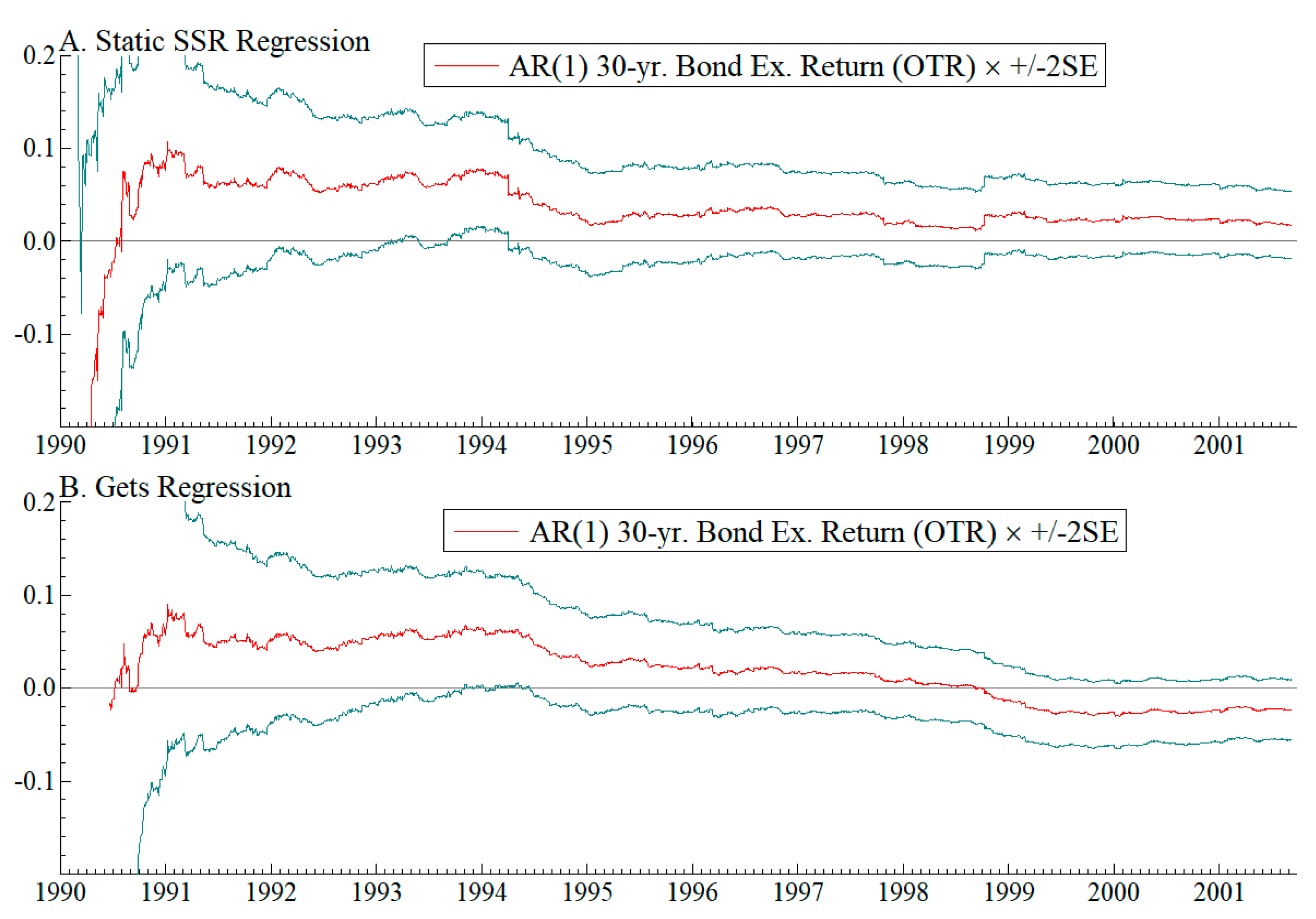
Appendix A.4. Recursive Stability Graphics

Appendix A.5. Recursive Parameters—Common Coefficients

Appendix A.6. Parameter Stability
| Panel A. SSR Models. | ||||
| OTR 30-Year | FTR 30-Year | OTR 10-Year | FTR 10-Year | |
| Hansen Instability Tests | ||||
| Variance | 1.779 ** | 2.184 ** | 0.770 * | 0.822 ** |
| Joint | 6.890 ** | 7.748 ** | 6.254 * | 6.241 * |
| Individual Instability Tests | ||||
| Constant | 0.037 | 0.035 | 0.043 | 0.043 |
| SS_AUTOS | 0.114 | 0.108 | 0.175 | 0.143 |
| SS_BUSINV | 0.103 | 0.086 | 0.185 | 0.138 |
| SS_CAPACIT | 0.460 | 0.381 | 0.470 | 0.485 * |
| SS_CONFIDN | 0.093 | 0.090 | 0.101 | 0.099 |
| SS_CONSTRC | 0.175 | 0.218 | 0.247 | 0.277 |
| SS_CPI | 0.054 | 0.054 | 0.054 | 0.054 |
| SS_CPIXFE | 0.063 | 0.059 | 0.079 | 0.082 |
| SS_DURGDS | 0.139 | 0.163 | 0.102 | 0.184 |
| SS_ECI | 0.074 | 0.080 | 0.111 | 0.110 |
| SS_GDP | 0.047 | 0.055 | 0.052 | 0.056 |
| SS_GDPPRIC | 0.125 | 0.115 | 0.237 | 0.215 |
| SS_GDSSERV | 0.148 | 0.157 | 0.158 | 0.169 |
| SS_HREARN | 0.127 | 0.126 | 0.071 | 0.090 |
| SS_HSLS | 0.066 | 0.064 | 0.057 | 0.058 |
| SS_HSTARTS | 0.575 * | 0.572 * | 0.749 * | 0.671 * |
| SS_INDPROD | 0.329 | 0.175 | 0.311 | 0.292 |
| SS_LEI | 0.107 | 0.114 | 0.104 | 0.108 |
| SS_NAPM | 0.249 | 0.303 | 0.138 | 0.157 |
| SS_NONFARM | 0.157 | 0.146 | 0.138 | 0.134 |
| SS_PCE | 0.438 | 0.525 * | 0.508 * | 0.514 * |
| SS_PERSINC | 0.152 | 0.172 | 0.108 | 0.099 |
| SS_PPI | 0.175 | 0.165 | 0.226 | 0.189 |
| SS_PPIXFE | 0.488 * | 0.400 | 0.582 * | 0.534 * |
| SS_RETSLS | 0.455 | 0.383 | 0.548 * | 0.479 * |
| SS_RSXAUTO | 0.052 | 0.046 | 0.061 | 0.063 |
| SS_UNEMP | 0.082 | 0.104 | 0.080 | 0.076 |
| Panel B. Gets Models with Indicator Saturates Removed. | ||||
| OTR 30-Year | FTR 30-Year | OTR 10-Year | FTR 10-Year | |
| Hansen Instability Tests | ||||
| Variance | 1.862 ** | 2.254 ** | 0.862 ** | 0.920 ** |
| Joint | 3.150 ** | 3.771 ** | 1.900 | 2.069 |
| Individual Instability Tests | ||||
| SS_CONFIDN | 0.109 | 0.107 | 0.118 | 0.113 |
| SS_CPIXFE | 0.069 | 0.074 | 0.093 | 0.103 |
| SS_DURGDS | 0.176 | 0.205 | 0.121 | 0.191 |
| SS_ECI | 0.040 | 0.113 | ||
| SS_HREARN | 0.140 | 0.143 | 0.086 | 0.108 |
| SS_HSLS | 0.067 | 0.065 | 0.061 | 0.061 |
| SS_NAPM | 0.237 | 0.293 | 0.140 | 0.158 |
| SS_NONFARM | 0.164 | 0.153 | 0.145 | 0.140 |
| NEG_SS_ECI | 0.112 | 0.124 | ||
| POS_SS_ECI | 0.077 | |||
Appendix A.7. Scenario Analysis—Selected Downside Announcement Surprises (U.S. Treasury OTR > 20 Years)
| Scenario | Model | Const | Beta 1 | Beta 2 | Shock | SS | YhatDiff | Value | Loss | ||
|---|---|---|---|---|---|---|---|---|---|---|---|
| 1 | Gets | 0.000 | −0.32 | Nonfarm Payrolls | 3 | −0.95 | $ | 4,817,689 | $ | 46,256 | |
| SSR | 0.013 | −0.39 | Nonfarm Payrolls | 3 | −1.17 | $ | 4,807,091 | $ | 56,855 | ||
| Difference | 3 | 0.22 | $ | 10,599 | |||||||
| 2 | Gets | 0.000 | −0.07 | Hourly Earnings | 3 | −0.20 | $ | 4,854,461 | $ | 9485 | |
| SSR | −0.035 | −0.24 | Hourly Earnings | 3 | −0.75 | $ | 4,827,661 | $ | 36,285 | ||
| Difference | 3 | 0.55 | $ | 26,800 | |||||||
| 3 | Gets | 0.000 | −0.32 | −0.10 | Nonfarm Payrolls and | 3 | −1.26 | $ | 4,802,806 | $ | 61,140 |
| SSR | 0.013 | −0.39 | −0.24 | Hourly Earnings | 3 | −1.90 | $ | 4,771,633 | $ | 92,313 | |
| Difference | 3 | 0.64 | $ | 31,173 | |||||||
| 4 | Gets | 0.000 | −0.79 | ECI | 3 | −2.36 | $ | 4,749,400 | $ | 114,546 | |
| SSR | 0.013 | −0.32 | ECI | 3 | −0.93 | $ | 4,818,473 | $ | 45,473 | ||
| Difference | 3 | −1.42 | $ | (69,073) |
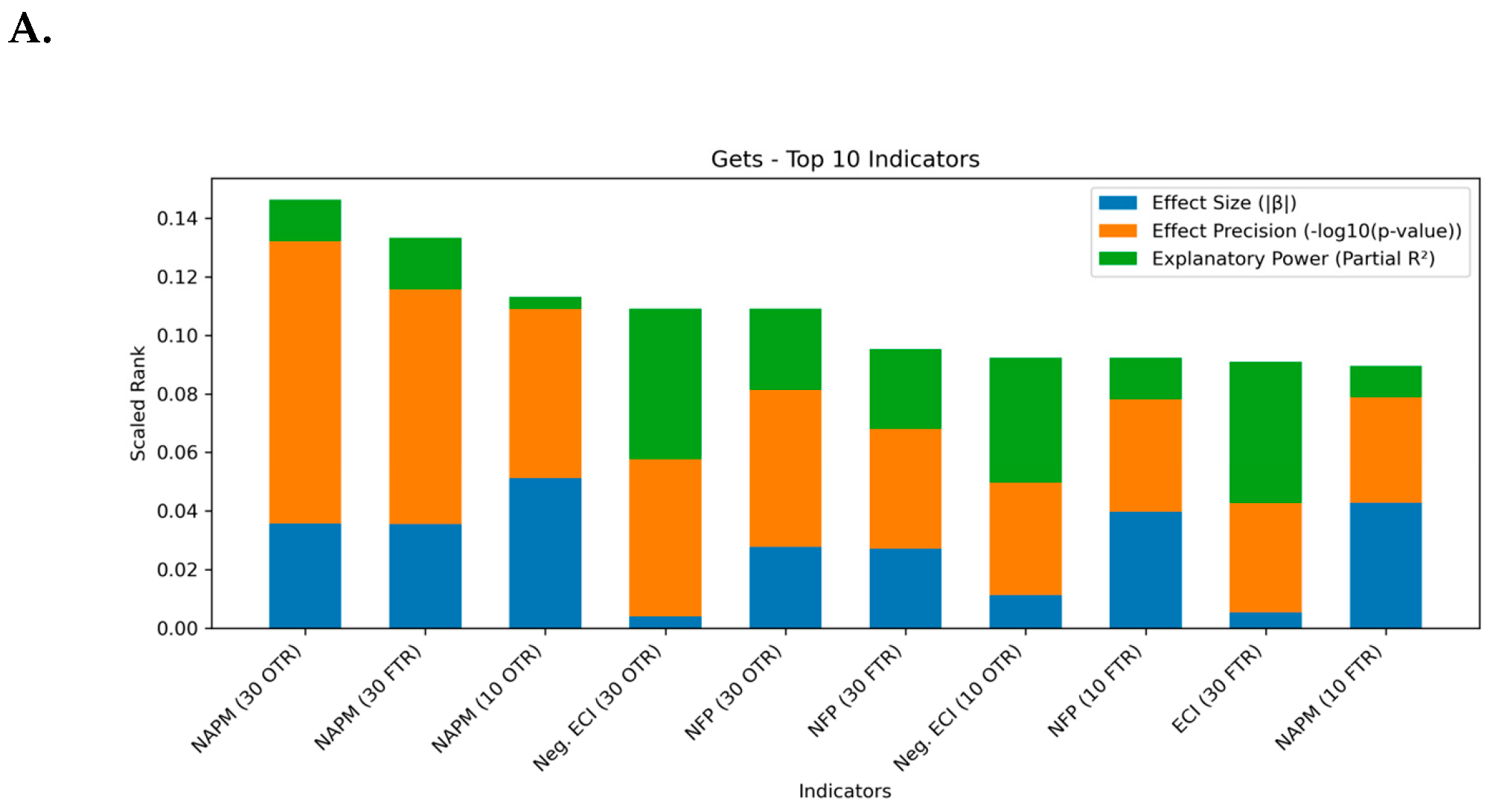
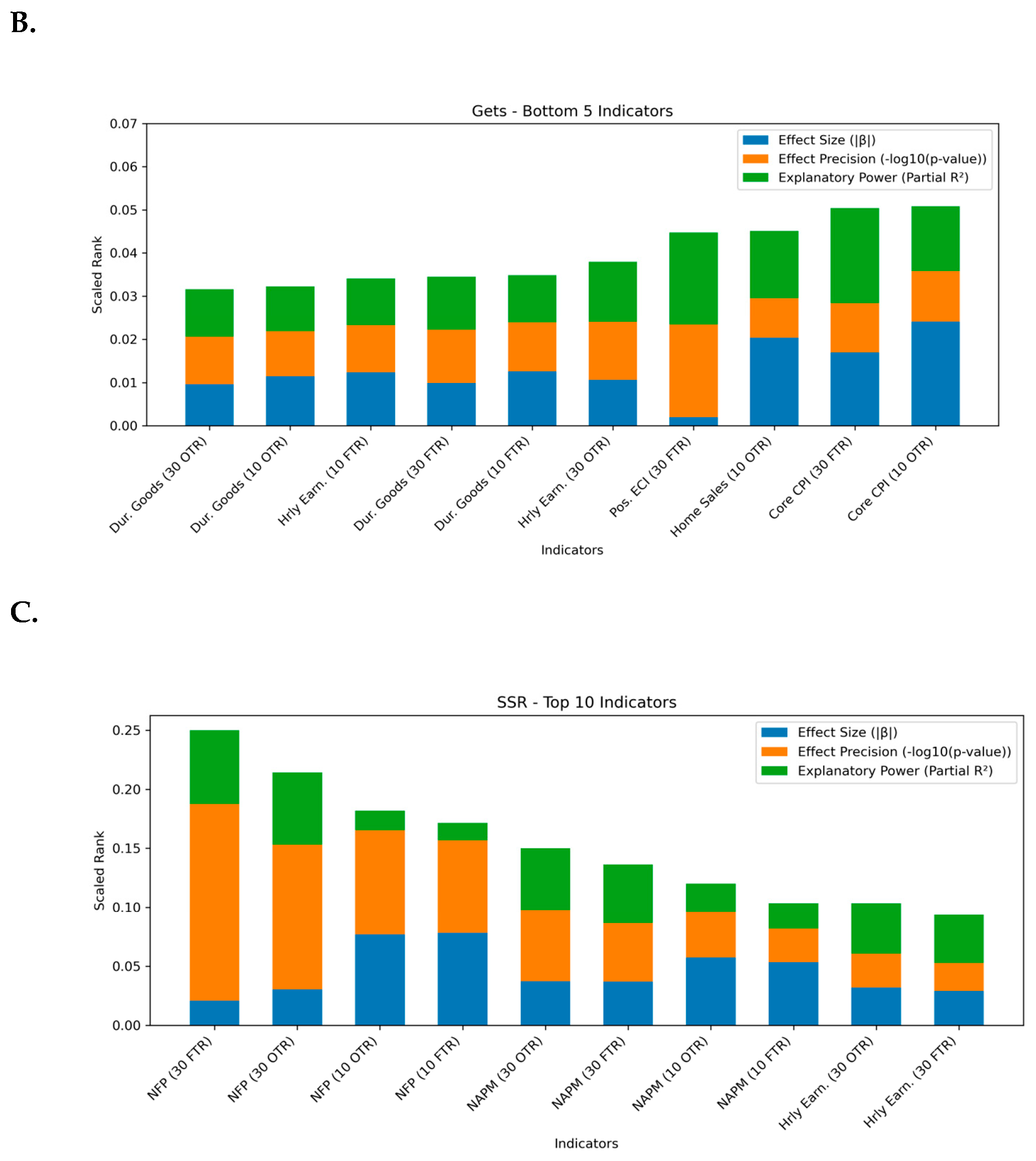
Appendix A.8. Effect Size, Precision, and Explanatory Power Analysis
| 1 | The Autometrics algorithm is discussed in detail in (Doornik, 2009) and the implementation is demonstrated in (Doornik & Hendry, 2022). |
| 2 | Indicator saturation is a statistical technique that enables models to account for structural breaks and outliers systematically, enhancing robustness and model accuracy. |
| 3 | Autometrics, part of the PcGive software suite, automates the model selection (Hendry & Doornik, 2014). |
| 4 | Details of Greenspan’s career can be found in (Sicilia & Cruikshank, 2000) and in (Greenspan, 2007). Note, a graphic depicting the path of US Treasury rates and spreads appears in Appendix A.1. |
| 5 | For examples of Greenspan’s pre-FRB scholarly works, see: (Greenspan et al., 1958; Greenspan, 1964, 1971, 1978, 1980; Hymans et al., 1973). |
| 6 | Other financial applications of Gets include: (Sucarrat & Escribano, 2012; Bekaert et al., 2012; Bekaert & Hoerova, 2014; Stillwagon, 2016, 2017; Frydman & Stillwagon, 2018; Frydman et al., 2020; Bekaert & Mehl, 2019; Bonnier, 2022; Gómez-Puig et al., 2023; Forest et al., 2024a; Marçal, 2024). |
| 7 | Here, ‘high-frequency’ refers to the Treasury return data, which are daily. While macro announcements are generally monthly or quarterly, their staggered timing across days produces continuous flows of information that can influence bond returns throughout each month. |
| 8 | For a more detailed description of the multiple path tree search used in the modern Autometrics package, see (Doornik, 2009). |
| 9 | See www.doornik.com (accessed on 1 May 2025) for additional details on the software. Given the large amount of data and candidate regressors, the computation can take several hours for each model. |
| 10 | The model selection literature often uses the term gauge to describe the false retention probability. |
| 11 | Computations were performed on an AMD Ryzen 5 laptop with 8 GB of RAM with 4 cores. Additional memory and processing power would likely improve computation time. |
| 12 | The Markov-switching models used here are standard two-state models with regime-dependent means and variances, estimated using PcGive. These models are intended to test whether regime-sensitive behavior is amplified or mitigated. |
| 13 | Notable studies using MMS Survey Data include: (T. Urich & Wachtel, 2012, 1984; T. J. Urich, 1982; Jain, 1988; Aggarwal et al., 1995; Li & Engle, 1998; Almeida et al., 1998; Balduzzi et al., 2001; Andersen et al., 2003, 2007; Ramchander et al., 2005; Kilian & Vega, 2012). |
| 14 | Stationarity of both the dependent variables (Treasury excess returns) and the standardized macroeconomic surprise regressors was confirmed using ADF-Fisher unit root tests. The null hypothesis of a unit root was rejected at the 1% level for all series. |
| 15 | See also: (Pasquariello & Vega, 2007) regarding the “on-the-run liquidity phenomenon”. |
| 16 | Recent work has rebranded the moniker to include Oxford, as the automation of model discovery methods were pioneered at Oxford University by Prof. Sir David F. Hendry and his coauthors. |
| 17 | Alternative Appendix A.1, available upon request. |
| 18 | Auto sales are subject to structural changes, particularly during labor strikes, and excluding them from retail sales may provide a better estimate of underlying consumer demand. |
| 19 | It is possible, but not tested here, that such key contemporaneous pairs may be best combined with an interaction term. |
| 20 | This is consistent with the concerns of (Smales, 2021), who provided supplementary regression for robustness for the same reason. Within the LSE/Oxford modelling framework, it is advised to reformulate the GUM to account for state dependencies and/or interactions of interest to explore this phenomena deeper. |
| 21 | Additional recursive stability diagnostics are given in Appendix A.5. |
| 22 | Visual inspection of terminal models suggests strong agreement amongst competing terminal models with respect to significant macro variables. Disagreement between competing models was observed to be concentrated in the adjacent dates of IIS and SIS alternatives. |
| 23 | See answer 5. |
| 24 | Autometrics allows the user to force retention of unrestricted fixed variables that are theoretically meaningful for evaluation. Therefore, we re-estimated Equation (2) with the first order lagged dependent variable fixed. |
| 25 | Although a rich literature on bond market reversals and momentum exists, I am not aware of any examples where Gets and saturation methods are used. See the following: (Khang & King, 2004; Zaremba & Kambouris, 2018; Li & Galvani, 2021; Zhang et al., 2021). |
| 26 | It is notable that the shrinkage of parameters under Gets is done post estimation, in contrast with penalty-based methods, such as Lasso. |
| 27 | It is also notable that the market did not appear to be affected by the anchoring bias suggested in the literature for several of the retained regressors. This implies that market participants adeptly adjust to the predictable bias of those economists participating in the MMS survey. |
References
- Aggarwal, R., Mohanty, S., & Song, F. (1995). Are survey forecasts of macroeconomic variables rational? The Journal of Business, 68(1), 99–119. [Google Scholar] [CrossRef]
- Aktas, N., de Bodt, E., & Levasseur, M. (2004). Heterogeneity effects from market interventions. The European Journal of Finance, 10(5), 412–436. [Google Scholar] [CrossRef]
- Almeida, A., Goodhart, C., & Payne, R. (1998). The effects of macroeconomic news on high frequency exchange rate behavior. The Journal of Financial and Quantitative Analysis, 33(3), 383–408. [Google Scholar] [CrossRef]
- Almon, S. (1965). The distributed lag between capital appropriations and expenditures. Econometrica, 33(1), 178–196. [Google Scholar] [CrossRef]
- Amin, S., & Tédongap, R. (2023). The changing landscape of treasury auctions. Journal of Banking & Finance, 148, 106714. [Google Scholar] [CrossRef]
- Andersen, T. G., Bollerslev, T., Diebold, F. X., & Vega, C. (2003). Micro effects of macro announcements: Real-time price discovery in Foreign exchange. American Economic Review, 93(1), 38–62. [Google Scholar] [CrossRef]
- Andersen, T. G., Bollerslev, T., Diebold, F. X., & Vega, C. (2007). Real-time price discovery in global stock, bond and foreign exchange markets. Journal of International Economics, 73(2), 251–277. [Google Scholar] [CrossRef]
- Balduzzi, P., Elton, E. J., & Green, T. C. (2001). Economic news and bond prices: Evidence from the U.S. treasury market. The Journal of Financial and Quantitative Analysis, 36(4), 523–543. [Google Scholar] [CrossRef]
- Balduzzi, P., & Moneta, F. (2017). Economic risk premia in the fixed-income markets: The intraday evidence. Journal of Financial and Quantitative Analysis, 52(5), 1927–1950. [Google Scholar] [CrossRef]
- Becker, W., Paruolo, P., & Saltelli, A. (2021). Variable selection in regression models using global sensitivity analysis. Journal of Time Series Econometrics, 13(2), 187–233. [Google Scholar] [CrossRef]
- Bekaert, G., Hodrick, R. J., & Zhang, X. (2012). Aggregate idiosyncratic volatility. Journal of Financial and Quantitative Analysis, 47(6), 1155–1185. [Google Scholar] [CrossRef]
- Bekaert, G., & Hoerova, M. (2014). The VIX, the variance premium and stock market volatility. Journal of Econometrics, 183(2), 181–192. [Google Scholar] [CrossRef]
- Bekaert, G., & Mehl, A. (2019). On the global financial market integration “swoosh” and the trilemma. Journal of International Money and Finance, 94, 227–245. [Google Scholar] [CrossRef]
- Bessembinder, H., Chan, K., & Seguin, P. J. (1996). An empirical examination of information, differences of opinion, and trading activity. Journal of Financial Economics, 40(1), 105–134. [Google Scholar] [CrossRef]
- Billio, M., Donadelli, M., Paradiso, A., & Riedel, M. (2017). Which market integration measure? Journal of Banking & Finance, 76, 150–174. [Google Scholar] [CrossRef]
- Blinder, A. S., Ehrmann, M., Fratzscher, M., De Haan, J., & Jansen, D.-J. (2008). Central Bank communication and monetary policy: A survey of theory and evidence. Journal of Economic Literature, 46(4), 910–945. [Google Scholar] [CrossRef]
- Bollerslev, T., Cai, J., & Song, F. M. (2000). Intraday periodicity, long memory volatility, and macroeconomic announcement effects in the US Treasury bond market. Journal of Empirical Finance, 7(1), 37–55. [Google Scholar] [CrossRef]
- Bonnier, J.-B. (2022). Forecasting crude oil volatility with exogenous predictors: As good as it Gets? Energy Economics, 111, 106059. [Google Scholar] [CrossRef]
- Bontemps, C., & Mizon, G. E. (2003). Congruence and encompassing. In Econometrics and the philosophy of economics: Theory-data confrontations in economics. Princeton University Press. [Google Scholar] [CrossRef]
- Bontemps, C., & Mizon, G. E. (2008). Encompassing: Concepts and implementation*. Oxford Bulletin of Economics and Statistics, 70(s1), 721–750. [Google Scholar] [CrossRef]
- Brockman, P., Chung, D. Y., & Pérignon, C. (2009). Commonality in liquidity: A global perspective. Journal of Financial and Quantitative Analysis, 44(4), 851. [Google Scholar] [CrossRef]
- Campbell, C. J., Kazemi, H. B., & Nanisetty, P. (1999). Time-Varying risk and return in the bond market: A test of a new equilibrium pricing model. The Review of Financial Studies, 12(3), 631–642. [Google Scholar] [CrossRef]
- Campbell, S. D., & Sharpe, S. A. (2009). Anchoring bias in consensus forecasts and its effect on market prices. Journal of Financial and Quantitative Analysis, 44(2), 369–390. [Google Scholar] [CrossRef]
- Campos, J., Hendry, D. F., & Krolzig, H.-M. (2003). Consistent model selection by an automatic Gets approach. Oxford Bulletin of Economics and Statistics, 65, 803–819. [Google Scholar] [CrossRef]
- Castle, J. L., Doornik, J., Hendry, D., & Pretis, F. (2015). Detecting location shifts during model selection by step-indicator saturation. Econometrics, 3(2), 240–264. [Google Scholar] [CrossRef]
- Castle, J. L., Doornik, J. A., & Hendry, D. F. (2013). Evaluating automatic model selection. Journal of Time Series Econometrics, 3(3), 1941–1928. [Google Scholar] [CrossRef]
- Choi, J. (2013). What drives the value premium?: The role of asset risk and leverage. Review of Financial Studies, 26(11), 2845–2875. [Google Scholar] [CrossRef]
- Chong, Y. Y., & Hendry, D. F. (1986). Econometric evaluation of linear macro-economic models. The Review of Economic Studies, 53(4), 671–690. [Google Scholar] [CrossRef]
- Chow, G. C. (1960). Tests of equality between sets of coefficients in two linear regressions. Econometrica, 28, 591–605. [Google Scholar] [CrossRef]
- Christie-David, R., Chaudhry, M., & Khan, W. (2002). News releases, market integration, and market leadership. Journal of Financial Research, 25, 223–245. [Google Scholar] [CrossRef]
- Connolly, R., & Stivers, C. (2005). Macroeconomic News, stock turnover, and volatility clustering in daily stock returns. Journal of Financial Research, XXVIII(2), 235–259. [Google Scholar] [CrossRef]
- Desboulets, L. D. D. (2018). A review on variable selection in regression analysis. Econometrics, 6(4), 45. [Google Scholar] [CrossRef]
- Dhrymes, P. J. (1971). Distributed lags: Problems of estimation and formulation. Holden-Day. [Google Scholar]
- Doornik, J. A. (2008). Encompassing and automatic model selection*. Oxford Bulletin of Economics and Statistics, 70(s1), 915–925. [Google Scholar] [CrossRef]
- Doornik, J. A. (2009). Autometrics. Oxford University Press. [Google Scholar] [CrossRef]
- Doornik, J. A., & Hansen, H. (2008). An omnibus test for univariate and multivariate normality*. Oxford Bulletin of Economics and Statistics, 70(s1), 927–939. [Google Scholar] [CrossRef]
- Doornik, J. A., & Hendry, D. F. (2022). PcGive 16. Timberlake Consultants. [Google Scholar]
- Ederington, L., & Lee, J. H. (1993). How markets process information: News releases and volatility. Journal of Finance, 48(4), 1161–1191. [Google Scholar] [CrossRef]
- Eijffinger, S. C. W., & Pieterse-Bloem, M. (2023). Eurozone government bond spreads: A tale of different ECB policy regimes. Journal of International Money and Finance, 139, 102965. [Google Scholar] [CrossRef]
- Engle, R. F. (1982). Autoregressive conditional heteroscedasticity with estimates of the variance of United Kingdom inflation. Econometrica, 50(4), 987–1007. [Google Scholar] [CrossRef]
- Engle, R. F., Hansen, M. K., & Lunde, A. (2012). And now, the rest of the News: Volatility and firm specific news arrival. CREATES Research Papers. Department of Economics and Business Economics. [Google Scholar]
- Epprecht, C., Guégan, D., Veiga, Á., & Correa da Rosa, J. (2019). Variable selection and forecasting via automated methods for linear models: Lasso/Adalasso and autometrics. Communications in Statistics—Simulation and Computation, 50(1), 103–122. [Google Scholar] [CrossRef]
- Ericsson, N. R. (2008). The fragility of sensitivity analysis: An encompassing perspective. Oxford Bulletin of Economics and Statistics, 70(s1), 895–914. [Google Scholar] [CrossRef]
- Ericsson, N. R. (2017). How biased are U.S. government forecasts of the federal debt? International Journal of Forecasting, 33(2), 543–559. [Google Scholar] [CrossRef]
- Ericsson, N. R., Dore, M. H. I., & Butt, H. (2022). Detecting and quantifying structural breaks in climate. Econometrics, 10(4), 33. [Google Scholar] [CrossRef]
- Fleming, M., & Remolona, E. (1999). Price formation and liquidity in the U.S. treasury market: The response to public information. Journal of Finance, 54(5), 1901–1915. [Google Scholar] [CrossRef]
- Forest, J. J. (2018). Essays in financial economics: Announcement effects in fixed income markets [Doctoral dissertation, University of Massachusetts-Amherst]. Available online: https://scholarworks.umass.edu/dissertations_2/1339 (accessed on 1 May 2025).
- Forest, J. J., Branch, B. S., & Berry, B. T. (2024a). Trading activity in the corporate bond market: A sad tale of macro-announcements and behavioral seasonality? Risks, 12(5), 80. [Google Scholar] [CrossRef]
- Forest, J. J., Chang, D. M., Doronkina, S., & Panahova, A. (2024b). Midas meets Fsher & Friedman: Assessing QTM as a short-term forecasting device. SUNY New Paltz. [Google Scholar] [CrossRef]
- Forest, J. J., & Doronkina, S. (2025). Rational expectations in housing markets: The case of survey forecasts. Working Paper. SUNY New Paltz. [Google Scholar] [CrossRef]
- Forest, J. J., & Mackey, S. (2023). The effect of treasury auction announcements on interest rates: 1990–1999. Academy of Economics and Finance Journal, 14, 1–10. [Google Scholar] [CrossRef]
- Forest, J. J., & Turner, P. (2013). Alternative estimators of cointegrating parameters in models with Non-stationary data: An application to US export demand. Applied Economics, 45(5), 629–636. [Google Scholar] [CrossRef]
- Frydman, R., Mangee, N., & Stillwagon, J. (2020). How market sentiment drives forecasts of stock returns. Journal of Behavioral Finance, 22(4), 351–367. [Google Scholar] [CrossRef]
- Frydman, R., & Stillwagon, J. R. (2018). Fundamental factors and extrapolation in stock-market expectations: The central role of structural change. Journal of Economic Behavior & Organization, 148, 189–198. [Google Scholar] [CrossRef]
- Gigante, G., Guarniero, P., & Pasini, S. (2024). Markovian analysis of U.S. Treasury volatility: Asymmetric responses to macroeconomic announcements. Economics Letters, 239, 111723. [Google Scholar] [CrossRef]
- Godfrey, L. G. (1978). Testing for higher order serial correlation in regression equations when the regressors include lagged dependent variables. Econometrica, 46(6), 1303–1310. [Google Scholar] [CrossRef]
- Govaerts, B., Hendry, D. F., & Richard, J.-F. (1994). Encompassing in stationary linear dynamic models. Journal of Econometrics, 63(1), 245–270. [Google Scholar] [CrossRef]
- Gómez-Puig, M., Pieterse-Bloem, M., & Sosvilla-Rivero, S. (2023). Dynamic connectedness between credit and liquidity risks in euro area sovereign debt markets. Journal of Multinational Financial Management, 68, 100800. [Google Scholar] [CrossRef]
- Granger, C. W. J., & Hendry, D. F. (2005). A dialogue concerning a new instrument for econometric modeling. Econometric Theory, 21(01), 278–297. [Google Scholar] [CrossRef]
- Greenspan, A. (1964). Liquidity as a determinant of industrial prices and interest rates. The Journal of Finance, 19(2), 159–169. [Google Scholar] [CrossRef]
- Greenspan, A. (1971). A model of capital expenditures and internal rates of return for the U.S. Economy. Business Economics, 6(3), 44–49. [Google Scholar]
- Greenspan, A. (1978). Inflation and economic activity. Business Economics, 13(3), 11–14. [Google Scholar]
- Greenspan, A. (1980). The great malaise. Challenge, 23(1), 37–40. [Google Scholar] [CrossRef]
- Greenspan, A. (2007). The age of turbulence. Penguin Books. [Google Scholar]
- Greenspan, A., Simpson, P. B., & Cutler, A. T. (1958). Discussion. The American Economic Review, 48(2), 171–177. [Google Scholar]
- Gürkaynak, R. S., Sack, B. P., & Swanson, E. T. (2007). Market-Based measures of monetary policy expectations. Journal of Business & Economic Statistics, 25(2), 201–212. [Google Scholar] [CrossRef]
- Hansen, B. E. (1992). Tests for parameter instability in regressions with 1(1) processes. Journal of Business & Economic Statistics, 10(3), 321–335. [Google Scholar] [CrossRef]
- Hendry, D. F. (1995). Dynamic econometrics. Oxford University Press. [Google Scholar] [CrossRef]
- Hendry, D. F. (2024). A Brief History of General-to-specific Modelling*. Oxford Bulletin of Economics and Statistics, 86, 1–20. [Google Scholar] [CrossRef]
- Hendry, D. F., & Doornik, J. A. (2014). Empirical model discovery and theory evaluation. MIT Press. [Google Scholar] [CrossRef]
- Hendry, D. F., & Krolzig, H. M. (1999). Improving on ‘Data mining reconsidered’ by K.D. Hoover and S.J. Perez. The Econometrics Journal, 2(2), 202–219. [Google Scholar] [CrossRef]
- Hendry, D. F., & Krolzig, H.-M. (2001). Computer automation of general-to-specific model selection procedures. Journal of Economic Dynamics and Control, 25, 831–866. [Google Scholar] [CrossRef]
- Hendry, D. F., & Krolzig, H.-M. (2005). The properties of automatic Gets modelling. The Economic Journal, 115(502), C32–C61. [Google Scholar] [CrossRef]
- Hendry, D. F., Pagan, A. R., & Sargan, J. D. (1984). Chapter 18 dynamic specification. In Z. Griliches, & D. Michael (Eds.), Handbook of econometrics (pp. 1023–1100). Intriligator. [Google Scholar] [CrossRef]
- Hess, D., & Orbe, S. (2013). Irrationality or efficiency of macroeconomic survey forecasts? Implications from the anchoring bias test*. Review of Finance, 17(6), 2097–2131. [Google Scholar] [CrossRef]
- Hoover, K. D., & Perez, S. (1999). Data mining reconsidered: Encompassing and the general-to-specific approach to specification search. Econometrics Journal, 2(2), 167–191. [Google Scholar] [CrossRef]
- Hymans, S. H., Greenspan, A., Shiskin, J., & Early, J. (1973). On the use of leading indicators to predict cyclical turning points. Brookings Papers on Economic Activity, 1973(2), 339–384. [Google Scholar] [CrossRef]
- Jain, P. C. (1988). Response of hourly stock prices and trading volume to economic News. Journal of Business, 61(2), 219–231. [Google Scholar] [CrossRef]
- Jones, C. M., Lamont, O., & Lumsdaine, R. L. (1998). Macroeconomic news and bond market volatility. Journal of Financial Economics, 47(3), 315–337. [Google Scholar] [CrossRef]
- Khang, K., & King, T. (2004). Return reversals in the bond market: Evidence and causes. Journal of Banking and Finance, 28, 569–593. [Google Scholar] [CrossRef]
- Kilian, L., & Vega, C. (2012). Replication data for: Do energy prices respond to U.S. macroeconomic News? A test of the hypothesis of predetermined energy prices. Harvard Dataverse. [Google Scholar] [CrossRef]
- Koyck, L. M. (1954). Distributed lags and investment analysis. North-Holland. [Google Scholar] [CrossRef]
- Krishnamurthy, A. (2002). The bond/old-bond spread. Journal of Financial Economics, 66(2–3), 463–506. [Google Scholar] [CrossRef]
- Li, L., & Engle, R. F. (1998). Macroeconomic announcements and volatility of treasury futures. UCSD Economics Discussion Papers. University of California San Diego. Available online: https://ssrn.com/abstract=145828 (accessed on 1 May 2025).
- Li, L., & Galvani, V. (2021). Informed trading and momentum in the corporate bond market*. Review of Finance, 25(6), 1773–1816. [Google Scholar] [CrossRef]
- Marçal, E. F. (2024). Testing rational expectations in a cointegrated VAR with structural change. International Review of Financial Analysis, 95, 103435. [Google Scholar] [CrossRef]
- Mizon, G. E., & Richard, J.-F. (1986). The encompassing principle and its application to testing non-nested hypotheses. Econometrica, 54(3), 657–678. [Google Scholar] [CrossRef]
- Muhammadullah, S., Urooj, A., Khan, F., Alshahrani, M. N., Alqawba, M., Al-Marzouki, S., & Zhu, P. (2022). Comparison of weighted lag adaptive Lasso with autometrics for covariate selection and forecasting using time-series data. Complexity, 2022, 2649205. [Google Scholar] [CrossRef]
- Pasquariello, P., & Vega, C. (2007). Informed and strategic order flow in the bond markets. Review of Financial Studies, 20(6), 1975–2019. [Google Scholar] [CrossRef]
- Phillips, P. C. B. (2005). Automated discovery in econometrics. Econometric Theory, 21(1), 3–20. [Google Scholar] [CrossRef]
- Pretis, F., Schneider, L., Smerdon, J. E., & Hendry, D. F. (2016). Detecting volcanic eruptions in temperature reconstructions by designed break-indicator saturation. Journal of Economic Surveys, 30(3), 403–429. [Google Scholar] [CrossRef]
- Ramchander, S., Simpson, M. W., & Chaudhry, M. K. (2005). The influence of macroeconomic news on term and quality spreads. The Quarterly Review of Economics and Finance, 45(1), 84–102. [Google Scholar] [CrossRef]
- Ramsey, J. B. (1969). Tests for specification errors in classical linear least-squares regression analysis. Journal of the Royal Statistical Society Series B: Statistical Methodology, 31(2), 350–371. [Google Scholar] [CrossRef]
- Sargan, J. D. (1959). The estimation of relationships with autocorrelated residuals by the use of instrumental variables. Journal of the Royal Statistical Society: Series B (Methodological), 21(1), 91–105. [Google Scholar] [CrossRef]
- Schirm, D. C. (2003). A comparative analysis of the rationality of consensus forecasts of U.S. Economic indicators. The Journal of Business, 76(4), 547–561. [Google Scholar] [CrossRef]
- Sicilia, D. B., & Cruikshank, J. L. (2000). The greenspan effect. McGraw-Hill. [Google Scholar]
- Smales, L. A. (2021). Macroeconomic news and treasury futures return volatility: Do treasury auctions matter? Global Finance Journal, 48, 100537. [Google Scholar] [CrossRef]
- Stillwagon, J. R. (2016). Non-linear exchange rate relationships: An automated model selection approach with indicator saturation. The North American Journal of Economics and Finance, 37, 84–109. [Google Scholar] [CrossRef]
- Stillwagon, J. R. (2017). TIPS and the VIX: Spillovers from financial panic to breakeven inflation in an automated, nonlinear modeling framework. Oxford Bulletin of Economics and Statistics, 80(2), 218–235. [Google Scholar] [CrossRef]
- Sucarrat, G., & Escribano, A. (2012). Automated model selection in finance: General-to-specific modelling of the mean and volatility specifications. Oxford Bulletin of Economics and Statistics, 74(5), 716–735. [Google Scholar] [CrossRef]
- Swanson, E. T. (2006). Have increases in federal reserve transparency improved private sector interest rate forecasts? Journal of Money, Credit, and Banking, 38(3), 791–819. [Google Scholar] [CrossRef]
- Tibshirani, R. (1996). Regression shrinkage and selection via the Lasso. Journal of the Royal Statistical Society: Series B (Methodological), 58(1), 267–288. [Google Scholar] [CrossRef]
- Tibshirani, R. (2011). Regression shrinkage and selection via the lasso: A retrospective. Journal of the Royal Statistical Society. Series B (Statistical Methodology), 73(3), 273–282. [Google Scholar] [CrossRef]
- Urich, T., & Wachtel, P. (1984). The effects of inflation and money supply announcements on interest rates. Journal of Finance, 39(4), 1177–1188. [Google Scholar] [CrossRef]
- Urich, T., & Wachtel, P. (2012). Market response to the weekly money supply announcements in the 1970s. The Journal of Finance, 36(5), 1063–1072. [Google Scholar] [CrossRef]
- Urich, T. J. (1982). The information content of weekly money supply announcements. Journal of Monetary Economics, 10(1), 73–88. [Google Scholar] [CrossRef]
- White, H. (1980). A heteroskedasticity-consistent covariance matrix estimator and a direct test for heteroskedasticity. Econometrica, 48(4), 817–838. [Google Scholar] [CrossRef]
- Zaremba, A., & Kambouris, G. (2018). The sources of momentum in international government bond returns. Applied Economics, 51, 848–857. [Google Scholar] [CrossRef]
- Zhang, W., Wang, P., & Li, Y. (2021). Bond intraday momentum. Journal of Behavioral and Experimental Finance, 31, 100515. [Google Scholar] [CrossRef]


| Range | Distribution | ||||||
|---|---|---|---|---|---|---|---|
| Indicators | Abbreviation | # Obs. | Avg. Abs. | Min. | Max. | Skewness | Kurtosis |
| SS | SS | SS | |||||
| Auto Sales | AUTOS | 199 | 0.78 | −2.92 | 2.47 | 0.17 | 3.05 |
| Business Inventories ab | BUSINV | 142 | 0.76 | −2.30 | 2.76 | 0.17 | 3.31 |
| Capacity Utilization ab | CAPACIT | 141 | 0.78 | −2.69 | 4.19 | 0.37 | 4.32 |
| Consumer Confidence ab | CONFIDN | 130 | 0.76 | −2.16 | 2.71 | 0.12 | 2.93 |
| Construction Spending ab | CONSTRC | 142 | 0.78 | −2.29 | 2.33 | −0.09 | 2.61 |
| Consumer Price Index r, ab | CPI | 130 | 0.74 | −2.48 | 2.48 | 0.24 | 3.35 |
| Core CPI (ex: food and energy) ab | CPIXFE | 141 | 0.66 | −1.68 | 3.36 | 1.07 | 4.46 |
| Durable Goods Orders nr, ab | DURGDS | 141 | 0.76 | −2.60 | 3.46 | 0.13 | 4.51 |
| Employment Cost Index | ECI | 30 | 0.83 | −2.03 | 3.04 | 0.50 | 3.41 |
| Gross Domestic Product | GDP | 138 | 0.77 | −2.19 | 3.10 | 0.59 | 3.48 |
| GDP Price Deflator | GDPPRIC | 117 | 0.63 | −3.79 | 1.89 | −1.33 | 5.95 |
| Goods and Services r, nb | GDSSERV | 142 | 0.79 | −2.40 | 3.79 | 0.29 | 3.78 |
| Hourly Earnings ab | HREARN | 142 | 0.82 | −2.22 | 2.66 | 0.02 | 2.39 |
| Home Sales nb | HSLS | 141 | 0.81 | −2.42 | 2.19 | −0.04 | 2.69 |
| Housing Starts r, ab | HSTARTS | 142 | 0.80 | −2.42 | 3.41 | 0.17 | 3.05 |
| Industrial Production nr, ab | INDPROD | 142 | 0.77 | −2.62 | 3.37 | 0.06 | 3.69 |
| Index of Lead. Econ. Ind. nr, ab | LEI | 142 | 0.72 | −4.43 | 3.16 | −0.22 | 5.68 |
| Nat. Assoc. of Purch. Mgrs. ab | NAPM | 142 | 0.80 | −2.65 | 2.25 | −0.05 | 2.81 |
| Nonfarm Payrolls r, nb | NONFARM | 143 | 0.77 | −2.53 | 3.30 | 0.01 | 3.43 |
| Personal Cons. Expenditures ab | PCE | 140 | 0.77 | −3.96 | 2.48 | −0.65 | 4.75 |
| Personal Income r, nb | PERSINC | 141 | 0.69 | −3.90 | 3.47 | 0.06 | 5.93 |
| Producer Price Index nr, ab | PPI | 143 | 0.77 | −2.88 | 3.24 | 0.20 | 3.60 |
| Core PPI (ex: food and energy) ab | PPIXFE | 143 | 0.71 | −5.22 | 2.61 | −0.89 | 7.38 |
| Retail Sales nr, ab | RETSLS | 142 | 0.78 | −4.02 | 2.68 | −0.35 | 4.07 |
| Retail Sales (ex: Auto Sales) ab | RSXAUTO | 142 | 0.72 | −3.36 | 2.52 | −0.52 | 4.40 |
| Unemployment Rate r, nb | UNEMP | 143 | 0.76 | −2.72 | 2.72 | 0.16 | 3.04 |
| 30-Year On-the-Run | 30-Year 1st Off-the-Run | ||||
|---|---|---|---|---|---|
| Indicators | Abbreviation | SSR | GETS | SSR | GETS |
| Coefficient | Coefficient | Coefficient | Coefficient | ||
| Constant | C | 0.105 * | 0.116 ** | ||
| Auto Sales | SS_AUTOS | −0.266 | −0.253 | ||
| Business Inventories | SS_BUSINV | 0.051 | 0.077 | ||
| Capacity Utilization | SS_CAPACIT | −0.474 | −0.498 | ||
| Consumer Confidence | SS_CONFIDN | −0.848 ** | −0.986 ** | −0.816 ** | −0.900 ** |
| Construction Spending | SS_CONSTRC | −0.058 | −0.041 | ||
| Consumer Price Index | SS_CPI | −0.247 | −0.253 | ||
| Core CPI (ex: food and energy) | SS_CPIXFE | −0.664 ** | −0.738 ** | −0.657 ** | −0.700 ** |
| Durable Goods Orders | SS_DURGDS | −0.680 ** | −0.529 ** | −0.675 ** | −0.617 ** |
| Employment Cost Index | SS_ECI | −1.174 ** | −1.156 ** | −2.557 ** | |
| Gross Domestic Product | SS_GDP | −0.122 | −0.102 | ||
| GDP Price Deflator | SS_GDPPRIC | −0.393 | −0.344 | ||
| Goods and Services | SS_GDSSERV | 0.030 | 0.050 | ||
| Hourly Earnings | SS_HREARN | −0.886 ** | −0.662 ** | −0.864 ** | −0.780 ** |
| Home Sales | SS_HSLS | −0.715 ** | −0.752 ** | −0.737 ** | −0.856 ** |
| Housing Starts | SS_HSTARTS | −0.057 | −0.030 | ||
| Industrial Production | SS_INDPROD | −0.021 | 0.087 | ||
| Index of Lead. Econ. Ind. | SS_LEI | −0.139 | −0.160 | ||
| Nat. Assoc. of Purch. Mgrs. | SS_NAPM | −1.138 ** | −1.355 ** | −1.085 ** | −1.287 ** |
| Nonfarm Payrolls | SS_NONFARM | −1.438 ** | −1.243 ** | −1.467 ** | −1.063 ** |
| Personal Cons. Expenditures | SS_PCE | −0.038 | −0.057 | ||
| Personal Income | SS_PERSINC | −0.318 | −0.320 | ||
| Producer Price Index | SS_PPI | 0.229 | 0.228 | ||
| Core PPI (ex: food and energy) | SS_PPIXFE | −0.582 ** | −0.622 ** | ||
| Retail Sales | SS_RETSLS | −0.697 * | −0.707 ** | ||
| Retail Sales (ex: Auto Sales) | SS_RSXAUTO | 0.085 | 0.090 | ||
| Unemployment Rate | SS_UNEMP | 0.244 | 0.262 | ||
| Negative ECI | NEG_SS_ECI | −2.726 ** | |||
| Positive ECI | POS_SS_ECI | 2.311 ** | |||
| sigma | 2.26 | 1.98 | 2.22 | 1.94 | |
| log-likelihood | −6523.74 | −6090.81 | −6468.16 | −6031.68 | |
| #. of observations | 2928 | 2927 | 2927 | 2927 | |
| RSS | 14,769.32 | 11,000.149 | 14,235.678 | 10,564.589 | |
| #. of parameters | 27 | 113 | 28 | 115 | |
| Adj. R2 | 0.064 | 0.309 | 0.065 | 0.313 | |
| Panel A. 30-Year Bond. | 30-Year OTR Bonds | 30-Year FTR Bonds | ||||||
|---|---|---|---|---|---|---|---|---|
| SSR | GETS | SSR | GETS | |||||
| Congruent | No | Yes | No | Yes | ||||
| AR 1-2 test | 0.5138 | 0.7579 | 0.8790 | 0.9120 | ||||
| ARCH 1-1 test | 0.0000 | ** | 0.4069 | 0.0000 | ** | 0.3816 | ||
| Normality test | 0.0000 | ** | 0.3021 | 0.0000 | ** | 0.9165 | ||
| Hetero test | 0.0058 | ** | 0.1181 | 0.0004 | ** | 0.0428 | * | |
| RESET23 test | 0.2951 | 0.2919 | 0.1642 | 0.3003 | ||||
| Panel B. 10-Year Note. | 10-Year OTR Notes | 10-Year FTR Notes | ||||||
| SSR | GETS | SSR | GETS | |||||
| Congruent | No | Yes | No | Yes | ||||
| AR 1-2 test | 0.0093 | ** | 0.1084 | 0.0125 | * | 0.1096 | ||
| ARCH 1-1 test | 0.0000 | ** | 0.8413 | 0.0000 | ** | 0.4914 | ||
| Normality test | 0.0000 | ** | 0.7605 | 0.0000 | ** | 0.8567 | ||
| Hetero test | 0.0002 | ** | 0.0101 | * | 0.0034 | ** | 0.0213 | * |
| RESET23 test | 0.0657 | 0.2033 | 0.0911 | 0.1548 | ||||
| Panel A. 30-Year Bond. | ||||||||||
| 30-Year OTR | 30-Year FTR | |||||||||
| A. | B. | C. | D. | E. | A. | B. | C. | D. | E. | |
| SSR | Gets | Gets | Gets | SSR | SSR | Gets | Gets | Gets | SSR | |
| Bias Corr. | Bias % | OV Bias % | Bias Corr. | Bias % | OV Bias % | |||||
| SS_CONFIDN | −0.85 | −0.99 | −0.98 | 1.0% | −13.3% | −0.82 | −0.90 | −0.90 | 0.0% | −8.9% |
| SS_CPIXFE | −0.66 | −0.74 | −0.72 | 2.8% | −8.3% | −0.66 | −0.70 | −0.67 | 4.5% | −1.5% |
| SS_DURGDS | −0.68 | −0.53 | −0.39 | 35.9% | 74.4% | −0.68 | −0.62 | −0.56 | 10.7% | 21.4% |
| SS_HREARN | −0.89 | −0.66 | −0.62 | 6.5% | 43.5% | −0.86 | −0.78 | −0.77 | 1.3% | 11.7% |
| SS_HSLS | −0.72 | −0.75 | −0.73 | 2.7% | −1.4% | −0.74 | −0.86 | −0.85 | 1.2% | −12.9% |
| SS_NAPM | −1.14 | −1.36 | −1.36 | 0.0% | −16.2% | −1.09 | −1.29 | −1.29 | 0.0% | −15.5% |
| SS_NONFARM | −1.44 | −1.24 | −1.24 | 0.0% | 16.1% | −1.47 | −1.06 | −1.06 | 0.0% | 38.7% |
| Panel B. 10-Year Note. | ||||||||||
| 10-Year OTR | 10-Year FTR | |||||||||
| SS_CONFIDN | −0.65 | −0.63 | −0.63 | 0.0% | 3.2% | −0.63 | −0.69 | −0.69 | 0.0% | −8.7% |
| SS_CPIXFE | −0.43 | −0.57 | −0.57 | 0.0% | −24.6% | −0.39 | −0.58 | −0.58 | 0.0% | −32.8% |
| SS_DURGDS | −0.42 | −0.39 | −0.36 | 8.3% | 16.7% | −0.41 | −0.40 | −0.42 | −4.8% | −2.4% |
| SS_HREARN | −0.58 | −0.63 | −0.63 | 0.0% | −7.9% | −0.56 | −0.41 | −0.38 | 7.9% | 47.4% |
| SS_HSLS | −0.52 | −0.49 | −0.47 | 4.3% | 10.6% | −0.55 | −0.61 | −0.61 | 0.0% | −9.8% |
| SS_NAPM | −0.82 | −0.88 | −0.88 | 0.0% | −6.8% | −0.77 | −0.77 | −0.77 | 0.0% | 0.0% |
| SS_NONFARM | −1.07 | −0.77 | −0.77 | 0.0% | 39.0% | −1.03 | −0.80 | −0.80 | 0.0% | 28.8% |
| Test | Model 1 vs. Model 2 | Model 2 vs. Model 1 |
|---|---|---|
| 30-Year OTR Bonds | ||
| Sargan | Chi2(106) = 771.62 [0.0000] ** | Chi2(20) = 41.113 [0.0036] ** |
| Joint Model | F(106,2794) = 9.556 [0.0000] ** | F(20,2794) = 2.0713 [0.0035] ** |
| sigma(M1) = 2.25673 | sigma(M2) = 1.97714 | sigma(Joint) = 1.96965 |
| 30-Year FTR Bonds | ||
| Sargan | Chi2(107) = 774.99 [0.0000] ** | Chi2(19) = 35.361 [0.0126] * |
| Joint Model | F(107,2793) = 9.5197 [0.0000] ** | F(19,2793) = 1.8721 [0.0123] * |
| Sigma(M1) = 2.21563 | sigma(M2) = 1.93829 | sigma(Joint) = 1.9326 |
| 10-Year OTR Notes | ||
| Sargan | Chi2(152) = 1029 [0.0000] ** | Chi2(20) = 27.436 [0.1234] |
| Joint Model | F(152,2748) = 9.9429 [0.0000] ** | F(20,2748) = 1.3755 [0.1227] |
| Sigma(M1) = 1.47236 | sigma(M2) = 1.21655 | sigma(Joint) = 1.2149 |
| 10-Year FTR Notes | ||
| Sargan | Chi2(154) = 1038.1 [0.0000] ** | Chi2(19) = 32.957 [0.0243] * |
| Joint Model | F(154,2746) = 9.9414 [0.0000] ** | F(19,2746) = 1.7435 [0.0239] * |
| Sigma(M1) = 1.41527 | sigma(M2) = 1.16836 | sigma(Joint) = 1.16539 |
Disclaimer/Publisher’s Note: The statements, opinions and data contained in all publications are solely those of the individual author(s) and contributor(s) and not of MDPI and/or the editor(s). MDPI and/or the editor(s) disclaim responsibility for any injury to people or property resulting from any ideas, methods, instructions or products referred to in the content. |
© 2025 by the author. Licensee MDPI, Basel, Switzerland. This article is an open access article distributed under the terms and conditions of the Creative Commons Attribution (CC BY) license (https://creativecommons.org/licenses/by/4.0/).
Share and Cite
Forest, J.J. The Effect of Macroeconomic Announcements on U.S. Treasury Markets: An Autometric General-to-Specific Analysis of the Greenspan Era. Econometrics 2025, 13, 24. https://doi.org/10.3390/econometrics13030024
Forest JJ. The Effect of Macroeconomic Announcements on U.S. Treasury Markets: An Autometric General-to-Specific Analysis of the Greenspan Era. Econometrics. 2025; 13(3):24. https://doi.org/10.3390/econometrics13030024
Chicago/Turabian StyleForest, James J. 2025. "The Effect of Macroeconomic Announcements on U.S. Treasury Markets: An Autometric General-to-Specific Analysis of the Greenspan Era" Econometrics 13, no. 3: 24. https://doi.org/10.3390/econometrics13030024
APA StyleForest, J. J. (2025). The Effect of Macroeconomic Announcements on U.S. Treasury Markets: An Autometric General-to-Specific Analysis of the Greenspan Era. Econometrics, 13(3), 24. https://doi.org/10.3390/econometrics13030024