Abstract
Applications of high-frequency data, including energy management, economics, and finance, frequently require time-series forecasting characterized by complex seasonality. Recognizing prevailing seasonal trends continues to be difficult, given that the majority of solutions depend on basic decomposition techniques. This study introduces a new approach employing periodograms from spectral density analysis to identify predominant seasonal periods. When analyzing hourly electricity consumption data from Brazil, we identified three significant seasonal patterns: sub-daily (6 h), half-daily (12 h), and daily (24 h). We assessed the predictive efficacy of the BATS, TBATS, and STL + ETS models using these seasonal periods. We performed data analysis and model fitting in R 4.4.1 and used accuracy metrics like MAE, MAPE, and others to compare the models. The STL + ETS model exhibited an enhanced performance, surpassing both BATS and TBATS in energy forecasting. These findings improve our understanding of multiple seasonal patterns, assist us in selecting dominating periods, provide new practical forecasting approaches for time-series analysis, and inform professionals seeking superior forecasting solutions in various fields.
Keywords:
time series; periodogram; energy; complex seasonality; forecasting; BATS; TBATS; STL models 1. Introduction
Time-series forecasting is becoming more and more important in fields such as energy, finance, economics, and healthcare, among others. Conventional models have a challenging time explaining these systems because of their complicated seasonal changes. Periodograms and other forms of spectral analysis have recently become reliable tools for identifying time series’ dominant frequencies, which allows for a more accurate representation of seasonal components in models.
Time-series analysis uses different types of models, such as non-seasonal, univariate seasonal, and multiple seasonal models, to predict future values of the time-series variable and figure out the underlying phenomenon by investigating the sequence of data. Based on the works of Shumway et al. (2000) and Sahu et al. (2022), the Autoregressive Integrated Moving Average (ARIMA) model is a common way to predict trends in univariate time-series data. However, it does not work for time series that have seasonal components. SARIMA extends ARIMA by allowing for the direct modeling of the seasonal component of the series.
Words in the seasonal component of the model involve seasonal backshifts, although they are otherwise similar to the non-seasonal components. In this way, the ARIMA model is altered. In the ARIMA and SARIMA models, we consider non-seasonal or relatively simple seasonal patterns such as seasonality in daily, weekly, monthly, quarterly, and annual time-series data. Yet, time series with a greater frequency and more seasonalities frequently show more intricate seasonal patterns (Ketabi et al., 2019; Borucka, 2023).
BATS and TBATS are advanced time-series forecasting models that handle complex seasonal patterns and nonlinear trends. BATS uses classic decomposition methods with ARMA error modeling, while TBATS models several seasonal cycles using trigonometric functions, making it ideal for high-frequency data with complex seasonality. STL (Seasonal and trend decomposition using Loess) is a robust non-parametric method that decomposes a time series into seasonal, trend, and residual components, providing flexibility and interpretability for evaluating time series with different seasonal patterns. These models forecast and comprehend time-series data, each having strengths based on data structure and complexity.
The specific goals of this study were that, by identifying the most dominant frequency, we would perform parameter estimation for time-series models with multiple seasonal periods (STL, BATS, and TBATS), carry out model selection and forecasting of the best fitted time-series model with multiple seasonality, and evaluate the forecasting performance of time-series models with multiple seasonal periods of hourly electricity consumption.
We use the periodogram that was discussed by Shumway and Stoffer (2016) to analyze spectral density and identify key seasonalities (sub-day, half-day, daily). Next, we develop a systematic method to select and incorporate these dominant seasonal periods into models. Then, we train and compare BATS, TBATS, and STL models with the selected seasonalities using standard accuracy metrics. So, the proposed spectral density-based method effectively identifies dominant seasonalities, improving model configurations. The work underlines the need of combining spectral analysis and advanced forecasting approaches to overcome the obstacles presented by high-frequency, complicated time-series analysis. The findings of this study are applicable to practitioners searching for reliable forecasting techniques in ever-changing scenarios.
The article is structured as follows: Section 2 presents a review of the existing literature and its scientific findings; Section 3 outlines the statistical methodology employed in this study; Section 4 delves into the results and gives a discussion; and Section 5 concludes this article by summarizing the key insights and implications.
2. Literature Review
In numerous time series, complex seasonality can be observed. According to the papers by De Livera et al. (2011), among the most prevalent complex seasonality types are “multiple nested seasonality periods”, numerous “non-nested and non-integer seasonality periods”, and “non-integer seasonality periods”. As they show, the current exponential smoothing models have several flaws when it comes to simulating complicated seasonality, including overparameterization and the incapacity to take into account “dual calendar effects and non-integer period effects”. They have introduced a new trigonometric framework for state-space modeling to solve these seasonal problems.
The “Box–Cox Transformation, ARMA Residuals, Trend, and Seasonality” (BATS) and “Seasonal Trigonometric, Box–Cox Transformation, ARMA Residuals, Trend, and Seasonality” (TBATS) models are used to predict complex seasonal time series with “multiple seasonal periods”, “high-frequency seasonality”, “non-integer seasonality”, and “dual-calendar effects”, as mentioned by De Livera et al. (2011) and Hyndman and Athanasopoulos (2021). The new model uses ARMA error correction and Fourier representations of the Box–Cox transformation with time-varying coefficients. We established a clear and comprehensive method for predicting complex seasonal time series on the basis of the assumption of Gaussian errors. Included in this strategy were mathematical expressions for interval predictions, point forecasts, and likelihood evaluation.
The seasonal models underlying the popular Holt–Winters multiplicative and additive approaches are the most widely utilized in the innovation state-space framework. As later suggested by De Livera et al. (2011), Hyndman and Athanasopoulos (2021), and Taylor (2003), the Holt–Winters technique can be expanded by adding a second seasonal component.
Numerous scholars have explored the concept of multiple seasonality in time-series forecasting. Ajeng (2019) discusses the forecasting performance of the TBATS model and compares its results with the STL (seasonal and trend decomposition using Loess) model, which accommodates multiple seasonal periods. The researcher employed R soft-ware 4.4.1 to analyze daily and weekly seasonality utilizing hourly power usage data sourced from PJM’s website. In conclusion, the STL model demonstrates a superior performance compared to the TBATS model. Using exponential smoothing time-series (ETS) models and the STL resilient approach for time-series decomposition is a good way to deal with complicated seasonal time-series data. We use Loess as a technique to forecast nonlinear relationships (Stefenon et al., 2023).
Three components make up the STL time-series filtering process: the trend, seasonality, and residual. Its straightforward design, comprising a sequence of Loess smoother applications, allows for fast computations, even for very large time series with several trends and seasonal smoothing, as well as the examination of the procedure’s properties, as cited by Cleveland et al. (1990) and Kranda and Samli (2022).
This is one method of addressing the overparameterization of the model parameters, and we noted from the works of De Livera et al. (2011) and Cleveland et al. (1990) that the MLEs of the parameters are not shown in the final fitted models for mathematical formulations. They also generalized their own models as the top-performing models for prediction. Furthermore, the STL model produces better forecasts than the TBATS model, according to Ajeng (2019). By using the hourly power consumption in Brazil from 2015 to 2022, this research study identifies the most dominant frequency and performs modeling and forecasting with many seasonal time-series periods to give a clear understanding in parameter estimations for the best fitted models and evaluate the forecasting abilities of the models with multiple seasonality.
An estimate of the demand for electricity is necessary for power system control and scheduling (Taylor & Snyder, 2012). Forecasts are necessary for lead times ranging from hourly to weekly. It is becoming more and more important for organizations to comprehend the advantages and disadvantages of various time-series models as they depend more and more on precise forecasts for operations and planning.
The ARIMA model was utilized to predict the peak demand for the subsequent 24 h, based on a continuous 168 h (one-week) dataset for five buildings. A preliminary analysis of these data was performed to ascertain the peak and off-peak hours for these buildings within the forthcoming 24 h. The hours fluctuated based on whether it was a weekday or the weekend (Alduailij et al., 2021).
Velasquez et al. (2022) stated that power forecasting helps determine electricity needs for system expansion, power plant availability based on installed capacity, and system functioning. The authors examined three time-series approximations and their combinations, using historical data from Brazil (SIN) and its subsystems to predict the electricity demand from 2021 to 2025. For the same time frame, the researchers also determined the percentage of incorrect EPE predictions. Using SIN and its subsystems’ historical data, the second method calculated the percentage of inaccurate power demand from 2014 to 2019. According to the results, the best strategy is regression with seasonality, and approximation errors can be decreased by combining time-series methods. In general, these results were used as a baseline to achieve our research objectives.
3. Materials and Methods
3.1. The Dataset
This research study utilized Brazil’s hourly electricity consumption (in megawatts) dataset from Kaggle (https://www.kaggle.com/datasets/arusouza/23-years-of-hourly-eletric-energy-demand-brazil, accessed on 1 March 2025) (Souza, 2022). It is a valuable resource for time-series analysis. We performed an extensive analysis of the last 7-year dataset (2015–2022) of Brazilian hourly electric energy demand to identify and model the different seasonal variations. Our literature study revealed the presence of multiple seasonal trends in a time series of power consumption data collected at hourly intervals.
3.2. A State-Space Model of Innovations for the Multiple Seasonal (MS) Processes
Multiple seasonal (MS) processes are included in the Innovation State-Space Model (ISSM), a flexible framework for modeling time-series data. This gives a method for breaking down the observed series into different elements, such as the trend, seasonality, and irregular fluctuations, while also enabling the insertion of further explanatory factors. The ISSM can be extended to account for these patterns when working with MS processes where multiple seasonal periods are present in the data. By using the model of De Livera et al. (2011) and the Springer Series in Statistics (2023), “an Innovation State-Space Model for multiple seasonal processes”, we can successfully represent the intricate interaction and patterns found in the data, which also enables the inclusion of other explanatory variables.
De Livera (2010) has shown that, given exponential smoothing, the BATS model is able to exceed the basic state-space model in terms of accuracy for prediction. But when seasonality is both complex and high frequency, the BATS model performs poorly. That is why De Livera et al. (2011) suggested the TBATS model. The trigonometric representation of seasonality terms can significantly lower the model’s parameters and increase its adaptability to complicated seasonality when there is a high frequency of seasonality.
3.2.1. BATS Model
De Livera et al. (2011) stated that “the nonlinear versions of the state space models underpin exponential smoothing”. The following is the modified form of the Double Seasonal (DS) model, which incorporates three seasonal patterns, ARMA errors, and a Box–Cox transformation (De Livera et al., 2011; Hyndman & Athanasopoulos, 2021):
since, in our data, , where refers to the value of Box–Cox transformation.
The general formulas for are given as follows:
These were formulated by De Livera et al. (2011) and Hyndman and Athanasopoulos (2021) and included only the three dominant frequencies in our dataset, namely, sub-daily (6 h), half-day (12 h), and daily (24 h) seasonalities. Refer to Section 3.2 of this article.
The local time frame at time t − 1 is given by
The period t short-term trend is given by
In our study, the dominant seasonal component in period t is given by
The ARMA errors (ARMA (5, 0)) process at time t in our study is given as
A Gaussian white-noise process characterized by a mean of zero (µ) and constant variance (σ2) is denoted as εt.
3.2.2. TBATS Model
De Livera et al. (2011) discuss the trigonometric representation of seasonal components, derived from the Fourier series, previously introduced by Harvey et al. (1997) and Herbert et al. (2021), as follows:
Model:
Box–Cox transformation: since, in our data, , where refers to the value of Box–Cox transformation, and is a series at time t.
The general formulas for are given as follows:
These were formulated by De Livera et al. (2011) and our new method of selection of the dominant frequencies.
The local time frame at time t − 1 is given by
The period t short-term trend is given by
As indicated in the BATS model above, the dominant seasonal component in period t is given by
An ARMA (p, q)—in our case, ARMA (3, 4)—process at time t is given as follows:
Seasonal part of the model:
In general, the method that we used to select the dominant seasonality is applied through the seasonal components , modeled using a trigonometric representation, as in the following formula:
where
= the dominant seasonal frequency identified from the periodogram.
and = coefficients to be estimated.
According to Herbert et al. (2021), the number of harmonics for the jth seasonal period is denoted as kj, with α, β, , and representing the smoothing parameters. The quantity of harmonics associated with the jth seasonal period is denoted as kj. A Gaussian white-noise process characterized by a zero mean (μ), and constant variance () is denoted by εt.
3.3. Multiple Seasonal (MS) Processes: A State-Space Model
State-space models (SSMs) can be extended to handle time-series data with multiple seasonal patterns. By incorporating multiple seasonal components into a state-space model, we can effectively capture the complex dynamics and interactions of different seasonal patterns in the data. This method makes it possible to model and forecast time series with numerous seasonal variations with greater accuracy (Puindi & Silva, 2021).
Seasonal and Trend Decomposition Utilizing the Loess (STL) Model
The STL model is a widely used method for breaking down a time series into its seasonal part, trend component, and remainder part, as mentioned in the study of Stefenon et al. (2023). The main STL model was designed to operate for just one seasonal period, but it can be extended to support various seasonal periods as well. By extending the STL model to cover multiple seasonal patterns, we obtained decomposed elements, which captured the numerous seasonal and trend patterns in our time-series data. Multiple seasonal time-series decomposition with the Exponential Smoothing Trend model is added to the STL model to develop MSTL + EST “Multiple seasonal time-series decomposition plus the Exponential Smoothing Trend”.
The equation for the MSTL + EST model can be described as follows:
In our data case, this formula is given as follows:
where
- —observed value.
- —local level, representing the overall average level or baseline.
- —local trend element, representing the rate of sloping.
- —ith seasonal component.
- n—number of seasonal periods.
- —error term, representing the random or unexplained component at time t.
3.4. Prediction
As stated by De Livera (2010) and Hyndman et al. (2005), let theta be a vector containing all of the parameters in a model that need to be estimated, n be the size, h be the forecasting length, and be a random variable that denotes the series’ future values given the model at the last observation , its estimated parameters, and the state vector. Assuming the error terms are Gaussian, the following formula determines the mean and variance, so must also be normally distributed.
as stated by Hyndman et al. (2005) and De Livera (2010)
where , with w′ and g representing the row and column vectors, respectively. At time t, the unobserved state vector is represented by , and a matrix is symbolized by F.
4. Results and Discussion
4.1. Preliminary Analysis
Our analysis examined 23 years of Brazilian hourly electric energy demand data (Souza, 2022). There are 201,318 observations. For the sake of simplicity in the statistical study, we utilized data from the last seven years (2015 to 2022) and rounded the observations to zero decimal places. Missed hourly observations were substituted with the average of the corresponding daily observations.
We carried out a thorough analysis of the Brazilian hourly electric energy demand dataset over the past 7 years to identify and model the various seasonal fluctuations. We anticipated several seasonal patterns, including sub-daily, half-day, and daily, would emerge due to the hourly nature of the data. Understanding the underlying dynamics of energy consumption and enhancing the accuracy of demand forecasts in the time-series field of research depend on accurately detecting these seasonalities.
Version 4.4.1 of the R program was used to analyze the data and fit the models (R Core Team, 2020). As indicated in Table 1, as an introduction, we performed a preliminary statistical analysis of the Brazilian data. From 1 January 2015 to 1 January 2023, the Brazilian electric power hourly consumption average was 64,670 MW per hour. During the specified period, the consumption ranged from 40,168 MW at the least to 90,120 MW at the maximum, with a standard deviation value of 9056. Naturally, seasonal variation accounts for a significant portion of the fluctuation. Strong seasonal patterns are frequently seen in the amount of electricity used, with lower levels of use during the summer months due to greater use of air conditioning and higher levels during the winter months for heating purposes. The data may become more complex as a result of several seasonal periods, which can increase variation. A simple representation of the time series illustrating Brazil’s hourly electricity usage from 1 January 2015 to 1 January 2023 is shown in Figure 1.

Table 1.
Hourly consumption of Brazilian electric power from 2015 to 2022 in megawatts.
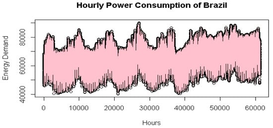
Figure 1.
Hourly power consumption of Brazil from 2015 to 2022.
The analyses’ findings are depicted in Figure 1. The plot has a definite seasonality and trend pattern over time. We modeled the time series before using the data for further analysis by considering or changing the seasonality term and trend patterns. Power usage peaked between the summer and winter months, as shown in Figure 1, because people use electricity more during these months for cooling and heating. We illustrated the pattern of seasonality in the data by using the ACF and spectrum analysis. A model of the time series was constructed by taking into account or making adjustments for the seasonality factor, as mentioned by De Livera et al. (2011), Shumway and Stoffer (2016), and Chudo (2022). This was carried out before the data were used for further research. It is our advice that researchers should make use of strategies that modify models and approaches in order to take into consideration the seasonality of the data.
4.2. Methods of Detecting the Multiple Seasonality in the Dataset
Due to a variety of operational, environmental, and human factors that affect energy use, hourly electric power consumption exhibits multiple seasonalities, including sub-daily, half-day, daily, weekly, and annual patterns. According to our dataset, the first three of these seasonalities occur for the following reasons:
- Sub-Daily: Due to a mix of environmental influences (such as temperature variations) and human activities (such as meals, industrial shifts, or midday routines), which result in recurring patterns throughout the day, the 6 h cycle most likely represents mid-cycle changes in demand.
- Half-Day: This cycle lasts for twelve hours. Daytime and nighttime energy power consumption varies significantly in many regional areas. In general, people’s energy consumption increases in the morning when they start their day and use appliances, and then again in the evening when they arrive home. A noticeable half-day seasonality results from these variations, peaking around breakfast and early evening.
- Daily: In this cycle, there are 24 h. Daily activities, like domestic operations, business processes, and working hours, follow a regular twenty-four-hour standard schedule. In general, the amount of electricity used rises throughout the day and drops at night. This produces an everyday cycle of activity: heating, cooling, and lighting changes in appliance usage.
Because of their close links to social, economic, and environmental cycles, these various seasonalities are essential in time series for estimating, modeling, and forecasting the demand for electricity.
4.2.1. Histogram
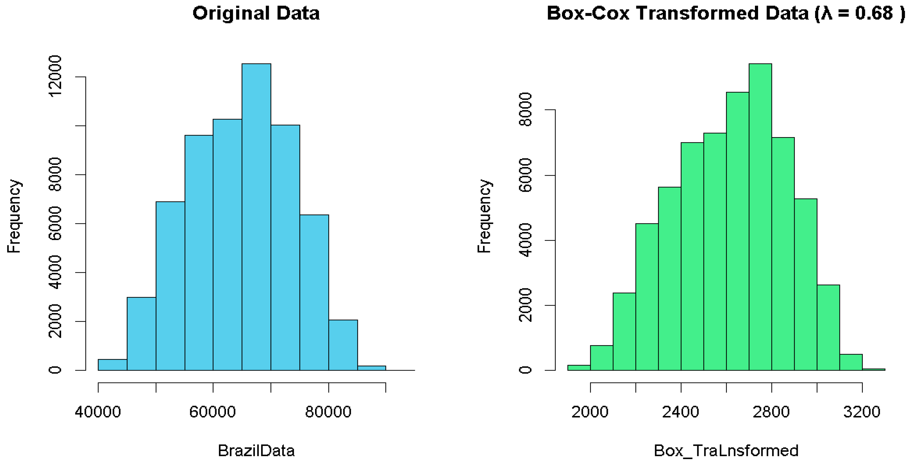
Examining the data distribution is a fundamental and essential aspect of data analysis. In our study, we examined the distribution of the original data and the Box–Cox transformed data, selecting the one that had a more normal distribution through the use of a histogram. We compared the normal distributions of the original and transformed data. Before that, we calculated the “optimal Box–Cox lambda” value using R soft-ware 4.4.1, which was 0.68. This was the minimum estimated value in the 95% CI. As shown in Figure 2, we used this (0.68) lambda value when plotting the histogram to check its normality and compared it with the first plot for the original data. Then, we used the Box–Cox transformed data for further analysis since they showed a better normal distribution than the original data.
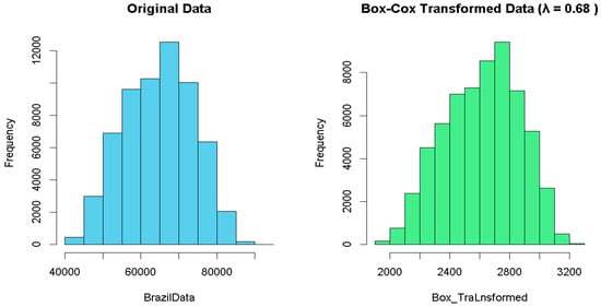
Figure 2.
Histogram of Brazil’s power consumption data from 2015 to 2022.
4.2.2. Plotting the Original, Box-Transformed, and Detrended Data Series for Comparison
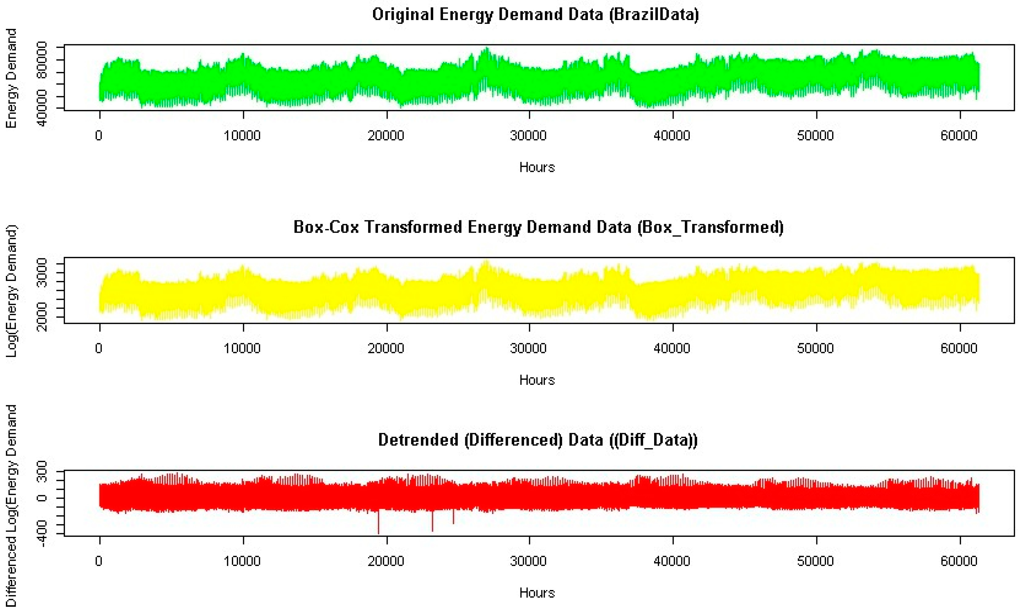
Verifying the data distribution, Figure 2 displays histograms for both the original and Box–Cox transformed data with lambda = 0.68. It indicates that the Box–Cox modified data were more normally distributed than the original data. Therefore, for our next investigation, we utilized the modified information rather than the original data. We examined the former to see if there was a trend and discovered some fluctuation. So, we took the Box–Cox transformed data’s initial difference, or de-trend. The plots of the original energy demand data, Box–Cox transformed energy demand data, and de-trended data are displayed in Figure 3. Lastly, we apply the de-trended data for multiple seasonality determination and model application in line with the Box–Cox transformation of the energy demand data.

Figure 3.
Original, Box-transformed, and detrended data series for comparison.
4.2.3. Periodogram
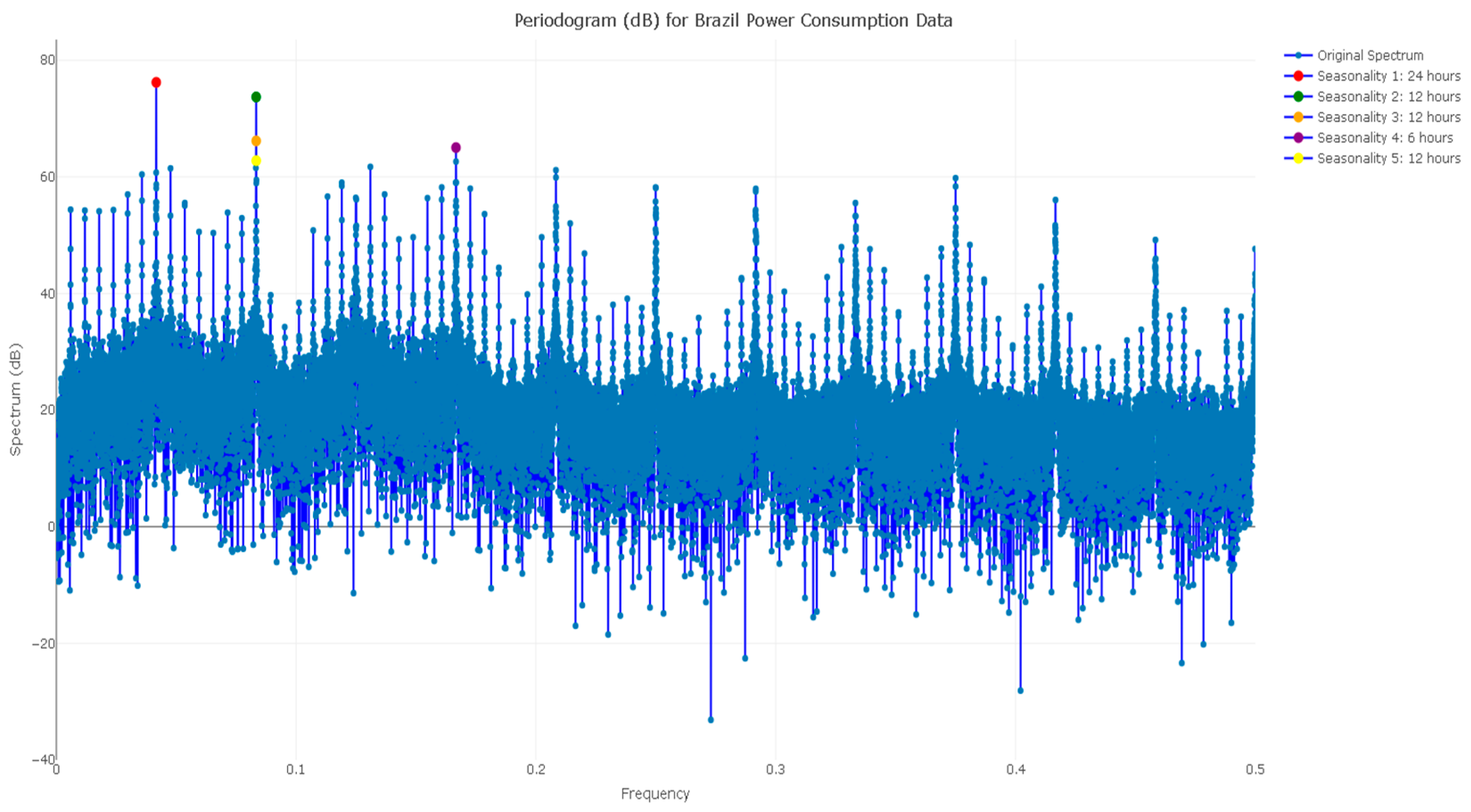
The second and most effective technique we employed to determine the peak periods in Brazil’s hourly power usage data was this one. Accurate time-series modeling, especially in energy demand forecasts, requires an understanding of multiple seasons. In order to model multiple seasonal time series, we utilized the periodogram produced through spectral density analysis to identify the top five most dominant frequencies. We can increase the forecasting accuracy by integrating patterns at different time periods after recognizing these seasonality components. The initial stage in the investigation is to compute the periodogram of the hourly power usage data. The periodogram provides an estimate of the spectral density by plotting the variance of the time series across several frequencies. We use the spec.pgram function to calculate the periodogram and convert the resulting power spectrum into decibels (dB) for simpler reading. To identify the most important seasonalities, we extract the top five dominating frequencies with the highest spectrum values. To facilitate visualization, these are shown in Figure 4.

Figure 4.
Periodogram (dB) of Brazil’s power consumption data from 2015 to 2022.
The periodogram shows several peaks, each of which corresponds to a different seasonal trend in the data. The periodogram values are ranked, allowing us to identify the frequencies with the highest spectra, which indicates the clearest repeating cycles in the data. The sub-daily (6 h cycle), half-day (12 h cycle), and daily (24 h cycle) seasonalities are the primary ones in energy use. The periodicities contribute most to the overall variation in the dataset when we plot the periodogram with markers for the top five dominating frequencies. The five most significant seasonal components in Brazil’s hourly power consumption statistics were successfully identified through this periodogram study. These frequencies were used to construct multiple seasonal time-series models, which accounted for the identified seasonal periods and improved the accuracy of energy demand forecasting in time series.
Figure 5 shows the STL decomposition (Data = Trend + Seasonal6 + Seasonal12 + Seasonal24 + Remainder) that we used for our further analysis after Box–Cox transformation and the first difference in the original data. It illustrates the breakdown of a time series for Brazilian data, verifying the presence of multiple seasonal patterns. As indicated in Figure 1, the series clearly shows seasonal patterns. Figure 5 decomposes the trend, seasonality, and remainder components of the series using functions in R soft-war 4.4.1. This mathematical formula can estimate the trend, seasonality, and irregular components of the time-series data. The decomposition of the transformed data reveals the presence of sub-daily (6 h cycle), half-day (12 h cycle), and daily (24 h cycle) seasonality in the data. As a result, we can observe the use of numerous or complicated seasonality techniques in our future modeling and forecasting, rather than relying on basic seasonality. To achieve the aim of this study, we apply the multiple time-series class, which manages several seasonality series. This allows us to specify every important frequency. Its flexibility enables the retention of non-integer frequencies within the series. Furthermore, the data in Figure 5’s fifth panel reveal a more pronounced and dominant period, which is the 24 h cycle. As the Springer Series in Statistics (2023) indicates, the data also appear to have an additive seasonal pattern, meaning that the fluctuation is unaffected by the time series’ level. As a result, we concentrated solely on additive models rather than multiplicative models. As we noted at the beginning of this analysis, the Brazil data contained a variety of seasonalities, including weekly and yearly patterns. However, in order to make model computations easier, only sub-daily, half-daily, and daily patterns were incorporated in this study based on the periodogram’s dominant frequency ranks.
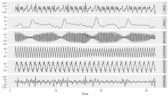
Figure 5.
Decomposition of a time series for sub-daily, half-day, and daily seasonalities.
4.3. BATS, TBATS, and STL Models
As mentioned by De Livera (2010) and Hyndman and Athanasopoulos (2021), many time series possess “multiple seasonality”, “complex seasonality”, “non-integer seasonality”, and multiple nested seasonality, in addition to simple seasonality. For basic seasonal patterns with short integer-valued periods, the majority of the current simple time-series models may be utilized, though using the most sophisticated forecasting models and techniques is crucial.
In this study, we applied forecasting time-series models like BATS “Box–Cox Transformation, ARMA Residuals, Trend, and Seasonality”, TBATS “Seasonal Trigonometric, Box–Cox Transformation, ARMA Residuals, Trend, and Seasonality”, and STL “Seasonal and Trend Decomposition utilizing the Loess Model” (De Livera et al., 2011; Ghane, 2020). The fundamental goal of these models is to use exponential smoothing to anticipate time series with multiple or complex seasonal trends. When using the Box–Cox transformation method, nonlinear data can be handled. BATS and TBATS models are simply the extensions of triple exponential smoothing (Holt–Winters) models, which were developed by De Livera et al. (2011) and cited by (Ajeng, 2019). We can consider these models with and without Box–Cox transformation, the trend, trend damping, the ARMA residual, non-seasonality, and harmonics used to model seasonal effects. Conversely, Taylor (2003) produced the Double Seasonal Holt–Winters model, which expanded upon the linear version of the Holt–Winters methodology.
We decomposed our data to check for multiple seasonality before forecasting the BATS, TBATS, and MSTL models. The calculated trend component indicated the presence of a pattern, as can be seen in Figure 1. The pattern in the trend source shows extra seasonality, which was not recorded because of longer natural periods in this data output. This revealed multi-seasonal data behavior. We segmented our data into a training set (Brazil-train) and testing set (Brazil-test) to facilitate comparison and forecasting analysis. The last seven years’ data (hourly power consumption in Brazil from 2015 to 2022) were chosen from the whole dataset. The last 912 h, or 38 days, of data were then utilized for data training, with the final week of data being used for data testing. Cyclical patterns in the modeling data were not shown since these occur usually after three years, according to time-series reports. The results from the application of multiple time-series BATS, TBATS, and STL models are presented herein. Because our original data decomposition was addictive and had no calendar fluctuation, we used the STL model in this study for multiple seasonality forecasting purposes.
In the following table, we compare the models (STL, BATS, and TBATS) on the energy power hourly consumption data for Brazil. They are evaluated by considering the least values of ME “Mean Error”, RMSE “Root Mean Square Error”, MAE “Mean Absolute Error”, MPE “Mean Percentage Error”, MAPE “Mean Absolute Percentage Error”, autocorrelation function (ACF1), and Theil’s U (a statistic used to evaluate whether or not a forecasting model is superior to naive forecasting). To evaluate how well the forecasting techniques performed on the provided data, we use MAPE since it is easy to understand. According to the least significant MAPE, which is indicated in Table 2, STL models showed better performances than BATS and TBATS models, with TBATS the second-best model. See Table 2 for more details.
Table 2.
Performance measurement values of the models.
4.3.1. Forecasting Time Series with BATS Model
As noted by De Livera (2010) and Herbert et al. (2021), the BATS model combines the “ARMA model for residuals”, “Box–Cox Transformation”, and the “Exponential Smoothing Method”. Time-series data are de-correlated using nonlinear data involving Box–Cox transformation and the ARMA model for residuals. The BATS model, when replacing the straightforward state-space model, can enhance forecast performance. However, the BATS model’s inability to suit complex and high-frequency seasonality is among its key weaknesses.
Data forecasting of Brazil’s hourly power consumption from BATS (1, {5, 0}, 0.998, {6, 12, 24}) is presented in Figure 6. The forecast generated by BATS fitted model is depicted in blue in Figure 6, whilst the grey hue indicates the 95% confidence interval of the forecast value.
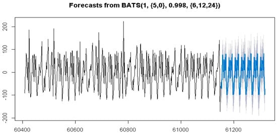
Figure 6.
Hourly electricity power consumption forecasting by the BATS model.
The basic approach reported in this subsection is to estimate the unknown parameters with a linear space model, like Box–Cox transformation parameters, ARMA coefficients, smoothing parameters, damping parameters, and so on. According to De Livera’s general formula, the BATS-fitted forecast model uses the following general formula in exponential smoothing methods: “BATS (1, {5, 0}, 0.998, {6, 12, 24})” and the estimated parameters listed in Table 3 with Sigma: 24.137 and AIC: 9779.919.
Table 3.
Parameter estimation for the BATS model.
In the BATS (1, {5, 0}, 0.998, {6, 12, 24}) model, the first value “1” represents the Box–Cox value. Accordingly, Box–Cox transformation is not suggested since this was considered with the lambda value 0.68 in the primary analysis of the data before the BATS model was applied. The ARMA error model was fitted, and the coefficient values were 5 and 0, indicating the fifth-order autoregressive and zero-order moving average coefficient values, respectively. Similarly, 0.998 represents the value of a damping parameter in the trend (the trend in the forecast will be reduced to 99.8 percent in each future period). The last set of values shows the sub-daily, half-daily, and daily seasonality periods, respectively.
Based on these, we could have fitted the following general BATS model for hourly energy power consumption in Brazil by using the De Livera et al. (2011) formula:
In our study, the Box–Cox transformation for and the first difference were applied. So,
where
4.3.2. Forecasting Time Series with the TBATS Model
Multiple seasonality is supported by both the BATS and TBATS models. The TBATS model, a variant of the BATS model, allows for many non-integer seasonality cycles in the time-series process. De Livera (2010) proposed the TBATS model, which incorporates the BATS model and trigonometric seasonality. More complex seasonality may be handled by the model thanks to the trigonometric representation of seasonality terms. Nonlinearity is handled using the Box–Cox transformation, and residual autocorrelation in the residuals is taken into consideration using the residual ARMA correction.
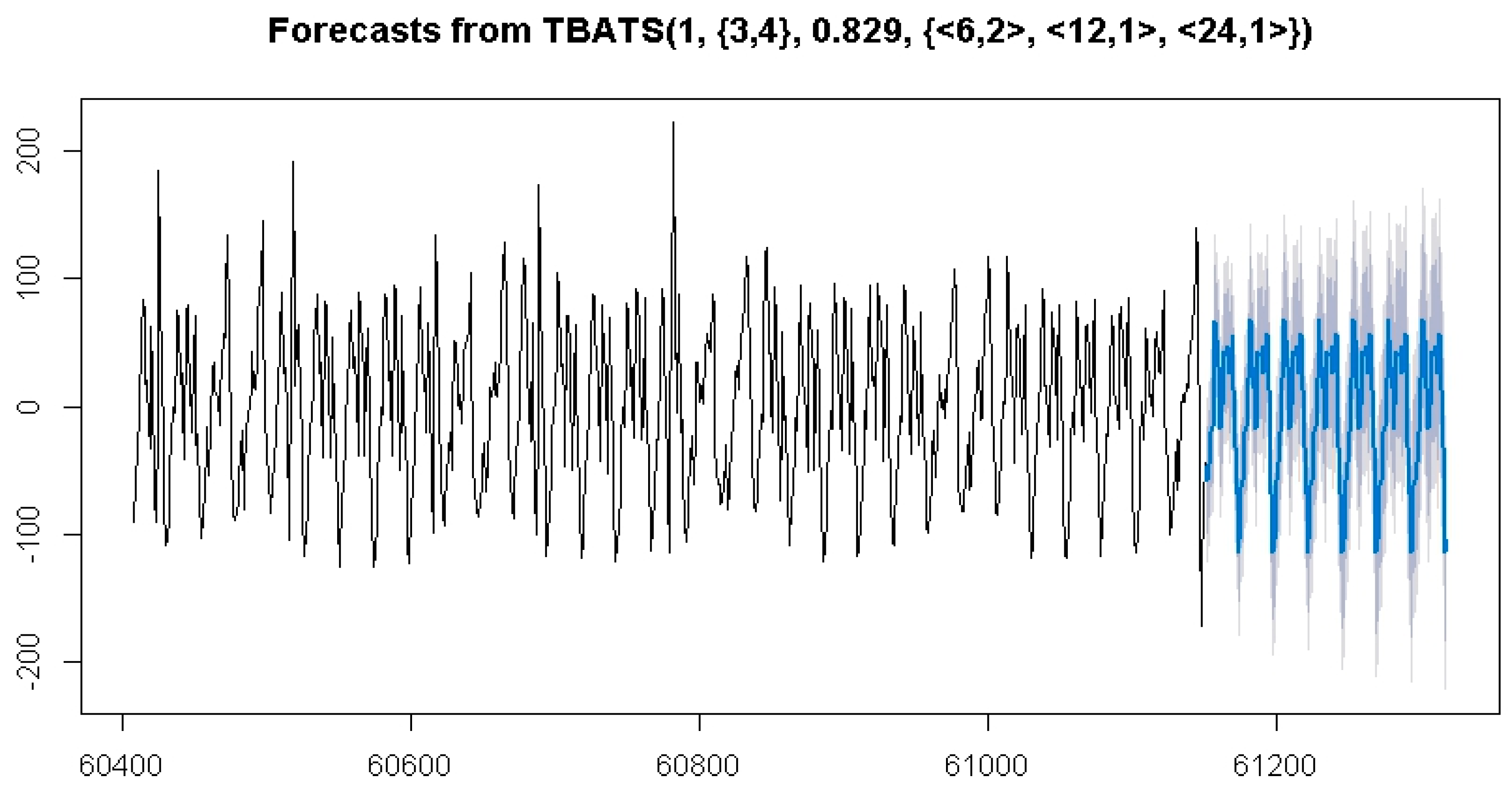
In Figure 7, the fitted model is designated TBATS [1, (3, 4), 0.829, (6, 2), (12, 1), (24, 1)] for hourly energy power consumption in Brazil. The value of lambda is one, which means that the Box–Cox transformation is not suggested because we already applied a transformation to the data before the application of the model. The damping parameter phi is 0.829, meaning that the trend will be dampened (the trend in the forecast will be reduced to 82.9% in each future period). The ARMA error was modeled as an ARMA (3, 4) process. The ARMA error model was fitted, and the values of the coefficients were 3 and 4, indicating the third-order autoregressive and fourth-order moving average coefficient values, respectively. The numbers 6, 12, and 24 represent the seasonal periods used in the model, which are sub-daily, half-day, and daily, with corresponding numbers of seasonal harmonics 2, 1, and 1, respectively, of Fourier terms used for each seasonality in the time series. This interpretation holds similarly with the BATS fitted model, except in the case of Fourier terms. In Figure 7, the blue color represents the forecast for TBATS fitted model, while the grey color indicates the 95% confidence interval of the forecast value.
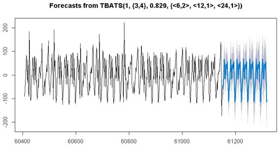
Figure 7.
Hourly electricity power consumption forecasting by the TBATS model.
The fitted forecast model, TBATS [1, (3, 4), 0.829, (6, 2), (12, 1), (24, 1)], takes its roots by using De Livera’s general formula and estimated parameters listed in Table 4 with Sigma: 28.643 and AIC: 9977.474.
Table 4.
Parameters estimation for the TBATS model.
Therefore, we could fit the following general TBATS model for hourly energy power consumption by using De Livera et al.’s (2011) formula:
Since we performed the Box–Cox transformation for on = 0.68,
where ;
4.3.3. Forecasting Time Series with the Multiple STL + ETS Model
Cleveland et al. (1990) introduced the STL model, a versatile and robust approach for decomposing time-series data. We used the Loess method to compute nonlinear relationships. In time series, the STL model was presented as a model for various seasonal processes. However, STL has significant shortcomings as well. For example, it only offers services for additive decomposition and does not automatically accommodate calendar variation.
The STL approach is Loess (LOcal regrESSion) smoothing, as Cleveland et al. (1990) illustrate. A time series can be filtered using STL to separate its trend, seasonal, and remaining components (Springer Series in Statistics, 2023). Additionally, Kranda and Samli (2022) noted the use of STL for long-term time series, significant trends, and seasonal smoothing. It is composed of a succession of the Loess smoother applications in a basic design that allows the study of the qualities’ simplicity.
The ETS (Error, Trend, Seasonal) model was defined by Hyndman and Khandakar (2008) and Jian Chai et al. (2021). In order to fit and anticipate the hourly electricity consumption from Brazilian data, the single exponential smoothing model ETS (A, N, N) was ultimately chosen based on the AIC. Errors are compounded in our model instance. According to researchers, algorithms with additive and multiplicative errors provide point forecasts that are identical but differ in terms of prediction intervals.
Smoothing parameter estimation of the exponential time-series model was performed as follows according to the outputs of the R software 4.4.1 with model ETS (A, N, N), alpha = 0.9999, I0 = −24.323, sigma = 23.7481, AIC = 7314.078, AICc = 7314.120, and BIC = 7327.146.
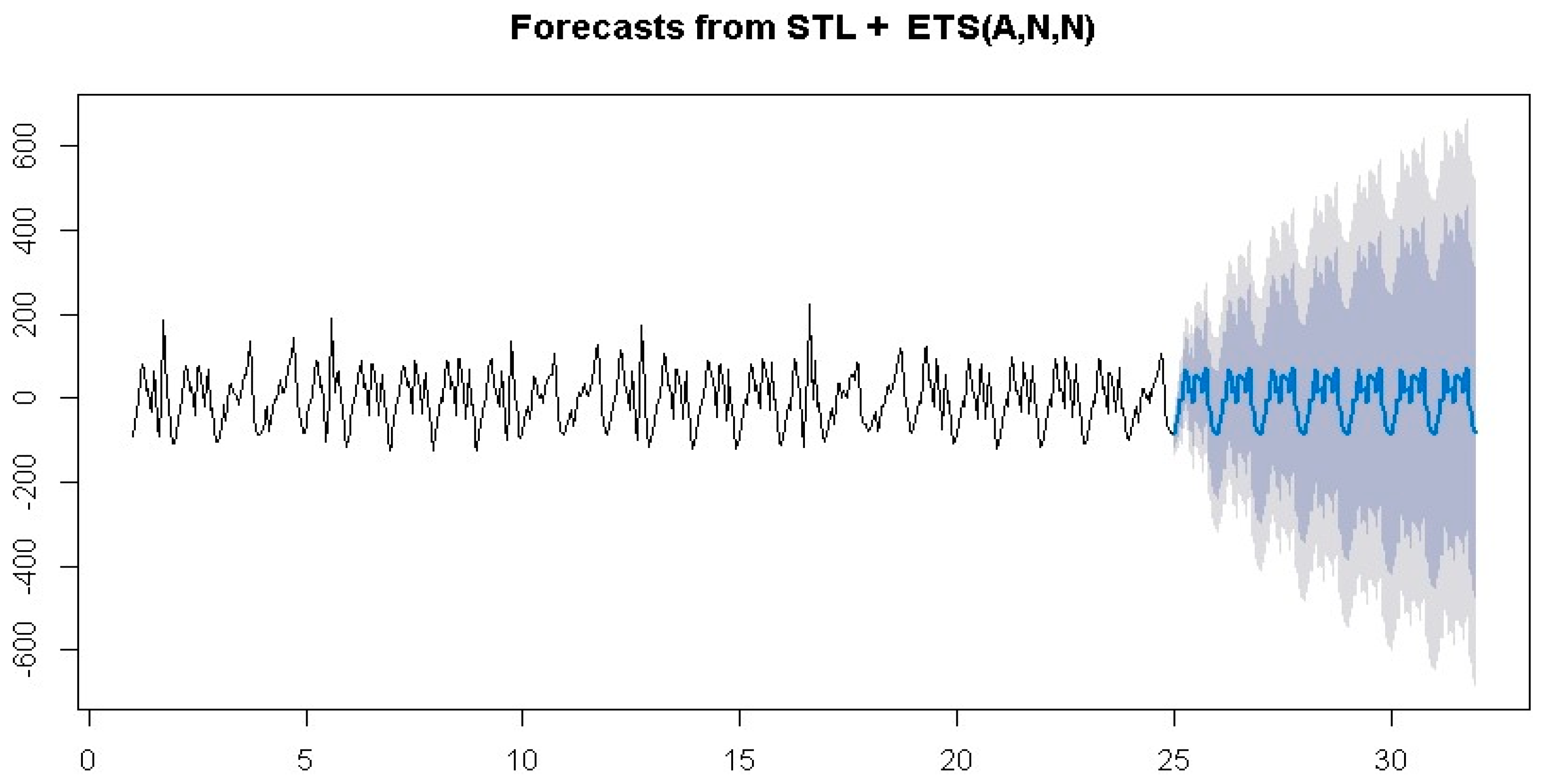
Figure 8 shows the forecasts for STL + ETS (A, N, N) of the hourly electricity power consumption according to Brazil’s data. Figure 8 displays the predicted value according to STL fitted model in blue, with the 95% confidence interval (CI) shown in grey and the 90% CI in silver.
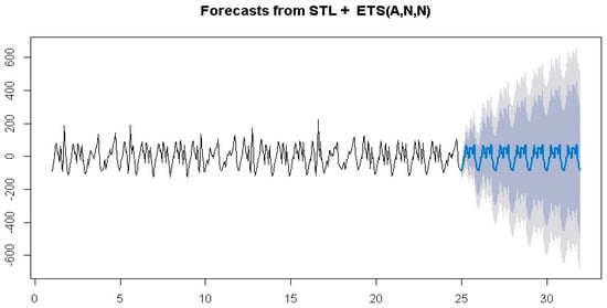
Figure 8.
Hourly electricity power consumption forecasting by the STL + ETS model. The blue part shows the forecasting and 95$ CI of it.
4.3.4. Checking the Different Performance Levels of Models by Charting Plots
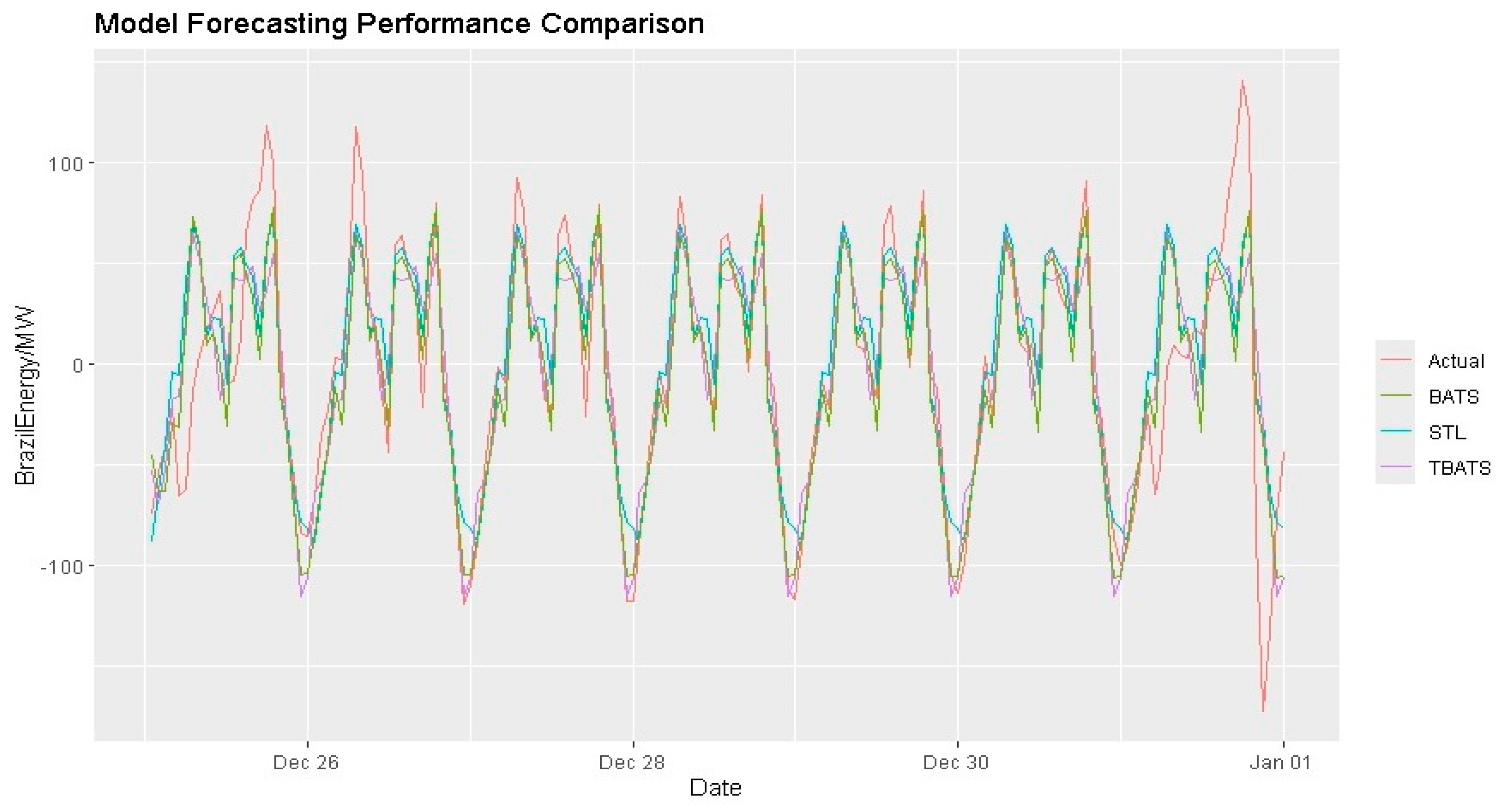
In the previous subsections, we demonstrated how the fitted BATS, TBATS, and STL models individually forecasted their performances. Next, we use a plot to illustrate the forecasting performance and compare the available models for multiple seasonal datasets in Brazil. This analysis employs the BATS, TBATS, and multiple STL models for the multi-seasonal data series. As indicated in Figure 9, the multiple STL (cyan color) models showed a better performance in forecasting the multi-seasonal Brazilian data than the BATS (olive color) and TBATS (purple color) models.
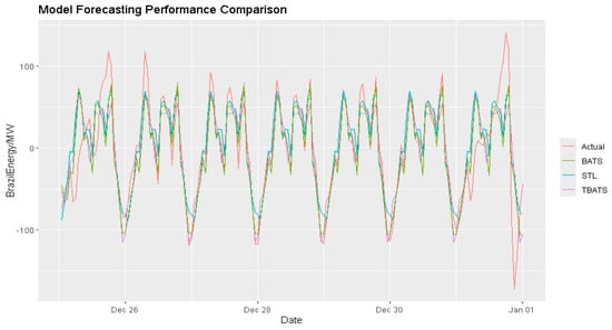
Figure 9.
Comparing the forecasting performances of the BATS, TBATS, and STL models.
5. Conclusions
We have demonstrated a new method for using spectral density analysis to detect multiple seasonalities. We selected sub-daily, half-daily, and daily seasonalities as the dominant frequencies. The original observations showed a combination of these three seasonal periods.
We fitted the models with their newly estimated parameters and compared the forecasting performances of multiple seasonal time-series models on hourly power consumption data in megawatts, sourced from a Brazilian database. We drew conclusions from the preliminary and further analyses of the dataset, along with the results and discussion of the data outputs. We applied three different seasonal time-series models: the TBATS model, the BATS model, and the multiple STL model. These complex seasonal time-series models also served as the basis for forecasting and comparisons.
We used the multiple time-series class, which is suitable for series with various seasonalities, rather than limiting the model to a single seasonality by seasonal difference. This made it possible for us to identify any frequency that might be significant while still having the flexibility to grasp integer and non-integer frequencies in the series.
We demonstrated well-fitted multi-seasonal models with statistically significant parameter estimations, and a description of every model’s mathematical formulas was given in the Discussion section. These, we hope, will aid others in building new fitting models for their fields and provide some guidance. Also, models based on the hourly power consumption data were compared and combined, determining the models with the lowest mean error, RME, MPE, MAPE, autocorrelation function, and Theil’s U statistic. Based on the indicated least values, the STL + ETS (A, N, N) models outperformed the TBATS and BATS models. Hence, the STL models showed a better performance in forecasting multi-seasonal data than the TBATS and BATS models.
In general, it is becoming more and more important for organizations to comprehend the advantages and disadvantages of various time-series models with different dominant frequencies, as they depend more and more on precise forecasts for operations and planning. The goal of the study was to identify the most dominant frequency and shed light on how well models of multiple seasonal periods performed when compared, paying particular attention to how well they could identify and forecast several seasonal components. This study provides practitioners with an efficient and methodical method for identifying dominant seasonal periods, estimating parameters, and developing robust time-series models. The findings have immediate implications for energy management systems, economics, finance, and other technical applications that require accurate projections of high-frequency data with complex seasonal patterns.
Author Contributions
Conceptualization, both authors; methodology, both authors; software, both authors; validation, both authors; formal analysis, S.B.C.; investigation, G.T.; resources, both authors; data curation, both authors; writing—original draft preparation, S.B.C.; writing—review and editing, both authors; visualization, S.B.C.; supervision, G.T.; project administration, both authors; funding acquisition, both authors. All authors have read and agreed to the published version of the manuscript.
Funding
This research was supported by the project TKP2021-NKTA of the University of Debrecen, Hungary. Project no. TKP2021-NKTA-34 has been implemented with support from the Ministry of Culture and Innovation of Hungary from the National Research, Development and Innovation Fund, financed under the TKP2021-NKTA funding scheme.
Data Availability Statement
Hourly energy demand data from Brazil were used https://www.kaggle.com/datasets/arusouza/23-years-of-hourly-eletric-energy-demand-brazil (accessed on 1 February 2025).
Conflicts of Interest
The authors declare no conflict of interest.
Abbreviations
The following abbreviations are used in this manuscript:
| BATS | Box–Cox Transformation, Autoregressive Moving Average Residuals, Trend, and Seasonality |
| TBATS | Seasonal Trigonometric, Box–Cox Transformation, Autoregressive Moving Average Residuals, Trend, and Seasonality |
| STL | Seasonal and Trend Decomposition utilizing the Loess Model |
| RMSE | Root Mean Squared Error |
| MAE | Mean Absolute Error |
| MPE | Mean Percentage Error |
| MAPE | Mean Absolute Percentage Error |
| ACF1 | Autocorrelation of Errors at Lag 1 |
| Theil’s U | Theil’s Unbiased Statistic |
| ETS | Exponential Smoothing |
| AIC | Akaike Information Criterion |
| ARIMA | Autoregressive Integrated Moving Average |
| SARIMA | Seasonal Autoregressive Integrated Moving Average |
| MSTL | Multiple Seasonal and Trend Decomposition utilizing the Loess Model |
| dB | Decibels |
| ACF | Autocorrelation Function |
| MW | Megawatt |
| MS | Multiple Seasonal |
| SSM | State-Space Model |
| DS | Double Seasonal |
| ISSM | Innovation State-Space Model |
| MLE | Maximum Likelihood Estimation |
| PJM | Pennsylvania–Jersey–Maryland |
| CI | Confidence interval |
References
- Ajeng, P. (2019). Forecasting time series with multiple seasonal. Available online: https://rpubs.com/AlgoritmaAcademy/multiseasonality (accessed on 5 July 2024).
- Alduailij, M. A., Petri, I., Rana, O., Alduailij, M. A., & Aldawood, A. S. (2021). Forecasting peak energy demand for smart buildings. The Journal of Supercomputing, 77(6), 6356–6380. [Google Scholar]
- Borucka, A. (2023). Seasonal methods of demand forecasting in the supply chain as support for the company’s sustainable growth. Sustainability, 15(9), 7399. [Google Scholar] [CrossRef]
- Chai, J., Zhao, C., Hu, Y., & Zhang, Z. G. (2021). Structural analysis and forecast of gold price returns. Journal of Management Science and Engineering, 6(2), 135–145. [Google Scholar] [CrossRef]
- Chudo, S. B. (2022, May 13–15). Multiplicative seasonal ARIMA modeling and forecasting of COVID_19 daily deaths in hungary. 10th International Conference on Bioinformatics and Computational Biology (ICBCB) (pp. 142–147), Hangzhou, China. [Google Scholar]
- Cleveland, R. B., Cleveland, W. S., McRae, J. E., & Terpenning, I. (1990). STL: A seasonal-trend decomposition. Journal of Official Statistics, 6(1), 3–73. [Google Scholar]
- De Livera, A. M. (2010). Automatic forecasting with a modified exponential smoothing state space framework. Monash Econometrics and Business Statistics Working Papers, 10(10), 6. [Google Scholar]
- De Livera, A. M., Hyndman, R. J., & Snyder, R. D. (2011). Forecasting time series with complex seasonal patterns using exponential smoothing. Journal of the American Statistical Association, 106(496), 1513–1527. [Google Scholar]
- Ghane, K. (2020, March 9–12). Big data pipeline with ML-based and crowd sourced dynamically created and maintained columnar data warehouse for structured and unstructured big data. 3rd International Conference on Information and Computer Technologies (ICICT) (pp. 60–67), San Jose, CA, USA. [Google Scholar]
- Harvey, A., Koopman, S. J., & Riani, M. (1997). The modeling and seasonal adjustment of weekly observations. Journal of Business & Economic Statistics, 15(3), 354–368. [Google Scholar]
- Herbert, Z. C., Asghar, Z., & Oroza, C. A. (2021). Long-term reservoir inflow forecasts: Enhanced water supply and inflow volume accuracy using deep learning. Journal of Hydrology, 601, 126676. [Google Scholar] [CrossRef]
- Hyndman, R. J., & Athanasopoulos, G. (2021). Forecasting: Principles and practice (3rd ed.). OTexts. Available online: https://otexts.com/fpp3/ (accessed on 5 August 2024).
- Hyndman, R. J., & Khandakar, Y. (2008). Automatic time series forecasting: The forecast package for R. Journal of Statistical Software, 27, 1–22. [Google Scholar]
- Hyndman, R. J., Koehler, A. B., Ord, J. K., & Snyder, R. D. (2005). Prediction intervals for exponential smoothing using two new classes of state space models. Journal of Forecasting, 24(1), 17–37. [Google Scholar] [CrossRef]
- Ketabi, R., Al-Qathrady, M., Alipour, B., & Helmy, A. (2019, November 25–29). Vehicular traffic density forecasting through the eyes of traffic cameras; a spatio-temporal machine learning study. 9th ACM Symposium on Design and Analysis of Intelligent Vehicular Networks and Applications (pp. 81–88), Miami Beach, FL, USA. [Google Scholar]
- Kranda, Y. T., & Samli, R. (2022). A novel clustering based algorithm to mitigate the demand of forecasting errors for newly deployed LTE cells with insufficient historical data. Computer Communications, 190, 190–200. [Google Scholar] [CrossRef]
- Puindi, A. C., & Silva, M. E. (2021). Dynamic structural models with covariates for short-term forecasting of time series with complex seasonal patterns. Journal of Applied Statistics, 48(5), 804–826. [Google Scholar] [PubMed]
- R Core Team. (2020). R: A language and environment for statistical computing. R Foundation for Statistical Computing. Available online: https://www.R-project.org/ (accessed on 10 January 2025).
- Sahu, M., Jhariya, D. C., Singh, R., Srivastava, I., & Mishra, S. K. (2022). Gis based spatial analysis and prediction of COVID-19 cases. In Journal of physics: Conference series (Vol. 2273, p. 012021). IOP Publishing. [Google Scholar]
- Shumway, R. H., & Stoffer, D. S. (2016). Time series analysis and its application with R examples (4th ed.). Springer Book. [Google Scholar]
- Shumway, R. H., Stoffer, D. S., & Stoffer, D. S. (2000). Time series analysis and its applications (Vol. 3, p. 4). Springer. [Google Scholar]
- Souza, A. (2022). 23 years of hourly electric energy demand (Brazil) data. Available online: https://www.kaggle.com/datasets/arusouza/23-years-of-hourly-eletric-energy-demand-brazil (accessed on 12 January 2025).
- Springer Series in Statistics (SSS). (2023). Available online: https://www.springer.com/series/692 (accessed on 17 July 2024).
- Stefenon, S. F., Seman, L. O., Mariani, V. C., & Coelho, L. D. S. (2023). Aggregating prophet and seasonal trend decomposition for time series forecasting of Italian electricity spot prices. Energies, 16(3), 1371. [Google Scholar] [CrossRef]
- Taylor, J. W. (2003). Short-term electricity demand forecasting using double seasonal exponential smoothing. Journal of the Operational Research Society, 54(8), 799–805. [Google Scholar]
- Taylor, J. W., & Snyder, R. D. (2012). Forecasting intraday time series with multiple seasonal cycles using parsimonious seasonal exponential smoothing. Omega, 40(6), 748–757. [Google Scholar]
- Velasquez, C. E., Zocatelli, M., Estanislau, F. B., & Castro, V. F. (2022). Analysis of time series models for Brazilian electricity demand forecasting. Energy, 247, 123483. [Google Scholar] [CrossRef]


Disclaimer/Publisher’s Note: The statements, opinions and data contained in all publications are solely those of the individual author(s) and contributor(s) and not of MDPI and/or the editor(s). MDPI and/or the editor(s) disclaim responsibility for any injury to people or property resulting from any ideas, methods, instructions or products referred to in the content. |
© 2025 by the authors. Licensee MDPI, Basel, Switzerland. This article is an open access article distributed under the terms and conditions of the Creative Commons Attribution (CC BY) license (https://creativecommons.org/licenses/by/4.0/).