
Explosive Episodes and Time-Varying Volatility: A New MARMA–GARCH Model Applied to Cryptocurrencies


Abstract
1. Introduction
2. Materials and Methods
2.1. MARMA()–GARCH() Processes
- GARCH Component.
2.1.1. Causal and Invertible Representation
2.1.2. Spectral Representations
- Higher-Order Periodogram.
2.2. Parameter Estimation and Identification
2.2.1. Two-Step Approach
- First Step (MARMA Identification).
- Fit a Causal–Invertible ARMA. Estimate the orders p and q (where and ) using information criteria (AIC, BIC) and significance tests. Treat the process as if it were causal and invertible, which allows for a standard ARMA() fit in the frequency or time domain (e.g., Whittle or Gaussian maximum likelihood).
- Redistribute Roots via Factorization. Once the ARMA() fit is obtained, factorize its polynomials and systematically explore all possible root allocations, corresponding to distinct causal/noncausal and invertible/noninvertible configurations. In practice, this step involves flipping certain roots inside/outside the unit disk (see Section 2.1).
- Select Final Representation. For each candidate, compute residual diagnostics such as higher-order spectral measures (Hecq & Velasquez-Gaviria, 2022, 2024; Velasco & Lobato, 2018) or a portmanteau-type test on and . The representation with the weakest remaining serial dependence (in both levels and squares) is chosen as the final MARMA specification.
- Second Step (GARCH(p,q) Estimation).
- Estimate GARCH. Using the final residual series from the identified MARMA model, estimate the parameters of a GARCH process (commonly GARCH in many financial applications).
- Whittle vs. MLE. We compare frequency-domain Whittle estimation (which typically requires higher-order moment assumptions) against time-domain maximum likelihood methods (which may hold under weaker moment conditions). Our Monte Carlo experiments suggest that MLE often exhibits smaller bias and variance, although Whittle remains a practical alternative if the required moments exist.
2.2.2. Estimation and Identification of the MARMA() Process
- Whittle Estimation.
- Redistributing Roots.
2.2.3. Spectral Identification Function
2.2.4. Portmanteau-Type Tests
2.2.5. Whittle Estimation for the GARCH() Model
- Whittle Criterion for GARCH.
2.2.6. Maximum Likelihood Estimation for the GARCH() Model
- Likelihood Function.
2.3. Detrending Methods
- Our Implementation.
2.3.1. Cubic Splines
2.3.2. Fourier Detrending
3. Results
3.1. Simulation Study
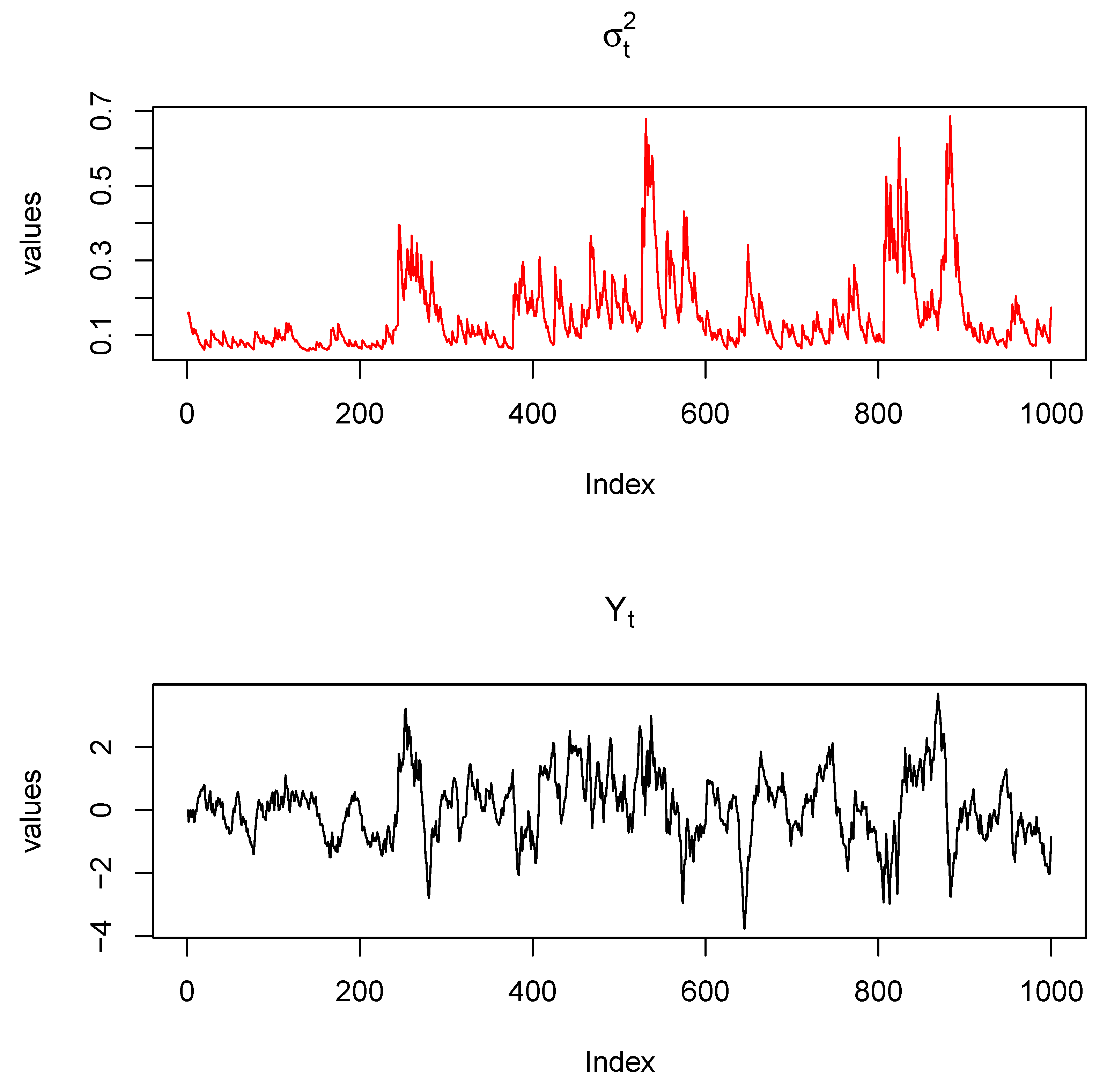
- Simulation Design.
- Generate Innovations: Draw an i.i.d. sequence of length T from a chosen distribution (e.g., Student’s t, skew-t, or exponential), with and .
- Simulate GARCH() Variance: Initialize . Recursively computeensuring remains strictly positive.
- Form GARCH Innovations:
- Fourier Representation of Residuals: Compute the DFT of :
- MARMA Transfer Function: Select parameters for the MARMA part. The frequency-domain transfer function is
- Construct the MARMA Process: Multiply the DFT of the innovations by the transfer function:
- Inverse DFT (Real Part):This final step yields , a realization from the specified MARMA–GARCH) process, provided stationarity and positivity conditions are met.
3.1.1. Whittle vs. Maximum Likelihood for Pure GARCH()
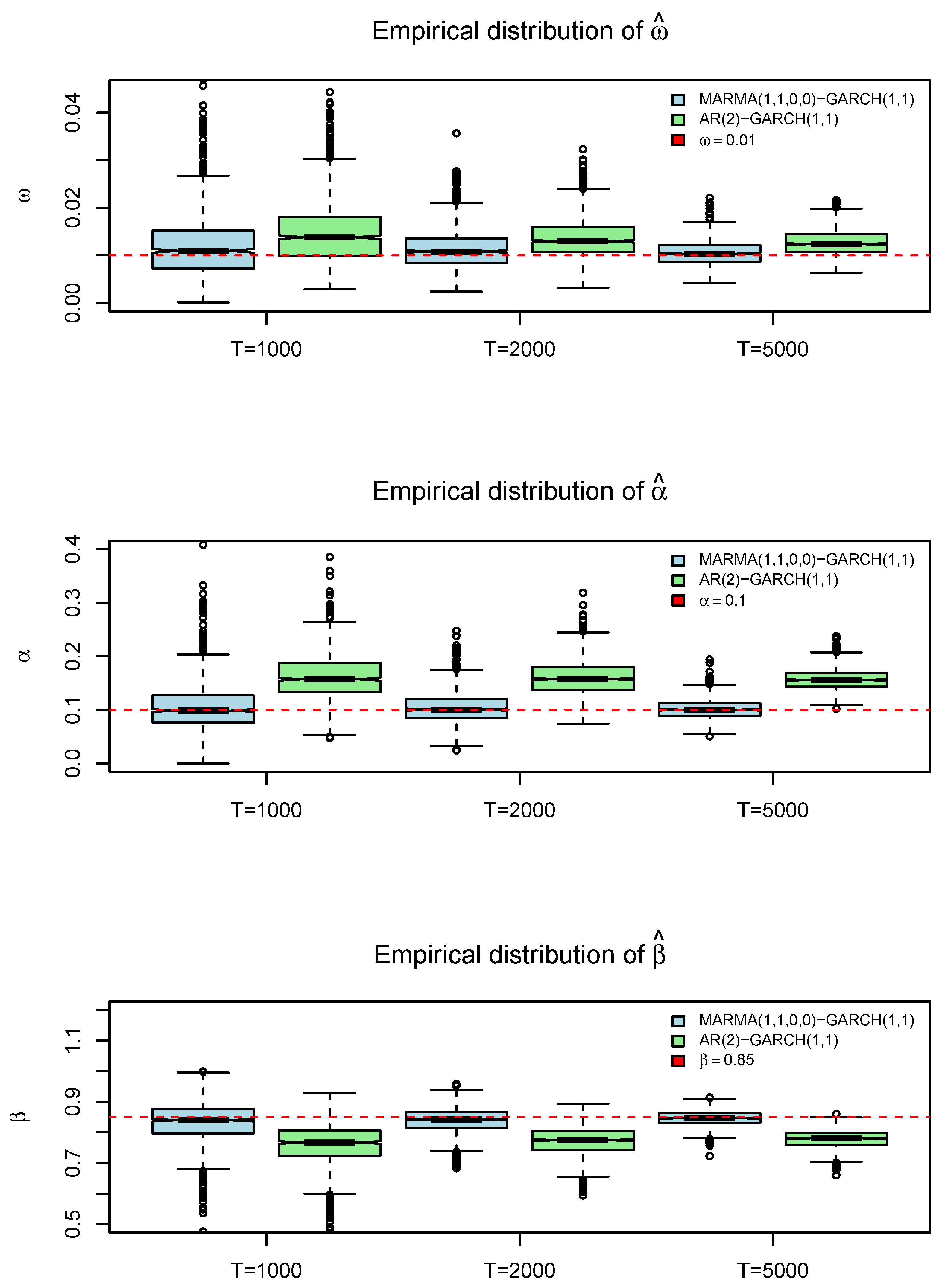
3.1.2. Estimating MARMA()–GARCH()
- Whittle vs. MLE for GARCH: Maximum likelihood estimation more accurately recovers the GARCH parameters, particularly in heavy-tailed environments, while Whittle estimation exhibits larger bias and RMSE.
- Importance of Correct MARMA Specification: Using a purely causal ARMA representation when the data are partially noncausal can distort the higher-order structure and lead to biased GARCH estimates. Correctly assigning the roots to causal/noncausal polynomials (as in a MARMA model) mitigates this issue.
3.2. Empirical Applications in Cryptocurrencies
- Detrending.
- Cubic Splines: Following Hall and Jasiak (2024), we employ a piecewise cubic spline with knots every 30 days. Additional experiments (e.g., quadratic vs. cubic, varying knot frequencies) suggested that a 30-day cubic spline balances flexibility with parsimony for these data.
- Fourier Filtering: We remove the lowest and highest 32 frequency components in the discrete Fourier transform of , corresponding to low-frequency trends and ultra-long cycles (Lobato & Velasco, 2022). This approach effectively zeroes out the first (and last) 32 harmonics before an inverse transform.
- Fitting MARMA–GARCH.
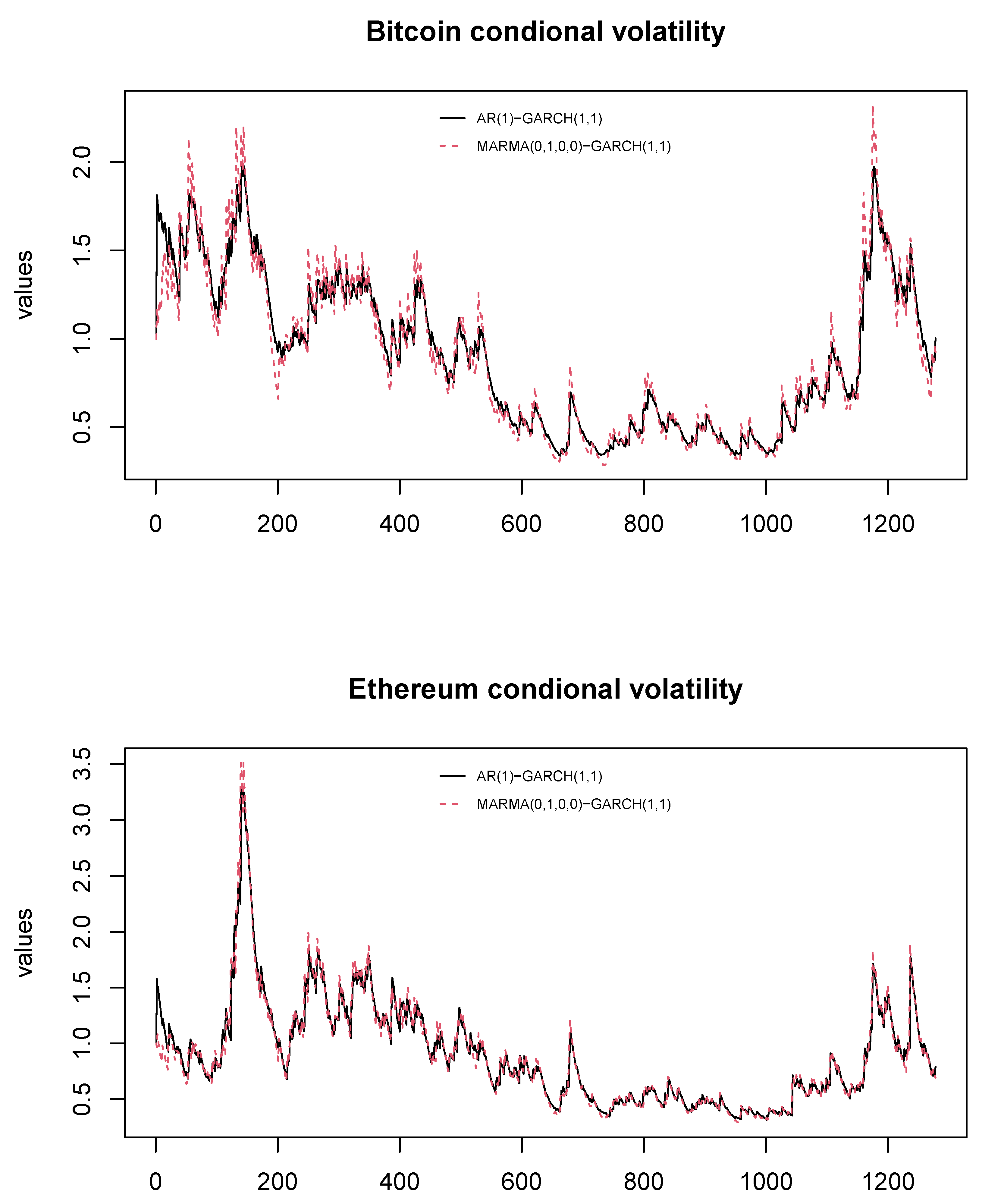
- GARCH(1,1) Estimation.
- Long-Run Volatility (ω): The noncausal MARMA–GARCH model consistently yields higher estimates of than the causal AR(1)–GARCH(1,1). Hence, ignoring noncausality may understate the baseline variance level.
- Reactivity to Shocks (α): The noncausal specification produces larger , suggesting that these cryptocurrencies exhibit more immediate responses to new information when future expectations (or bubble-like feedback) are accounted for.
- Volatility Persistence (β): Reflecting the stronger short-run reactivity, is lower in the MARMA–GARCH model, implying reduced persistence once the noncausal feedback is captured.
- Diagnostic Checks.
4. Discussion and Conclusions
- Practical and Societal Implications.
Author Contributions
Funding
Data Availability Statement
Conflicts of Interest
References
- Aguirre, A., & Lobato, I. N. (2024). Evidence of non-fundamentalness in OECD capital stocks. Empirical Economics, 67(2), 761–772. [Google Scholar]
- Ardia, D., Bluteau, K., & Rüede, M. (2019). Regime changes in Bitcoin GARCH volatility dynamics. Finance Research Letters, 29, 266–271. [Google Scholar] [CrossRef]
- Bazán-Palomino, W. (2022). Interdependence, contagion and speculative bubbles in cryptocurrency markets. Finance Research Letters, 49, 103132. [Google Scholar]
- Blasques, F., Koopman, S. J., & Mingoli, G. (2023). Observation-driven filters for time-series with stochastic trends and mixed causal non-causal dynamics (Tech. Rep.). Tinbergen Institute Discussion Paper. [Google Scholar]
- Blasques, F., Koopman, S. J., Mingoli, G., & Telg, S. (2024). A novel test for the presence of local explosive dynamics (Tech. Rep.). Tinbergen Institute Discussion Paper. [Google Scholar]
- Bollerslev, T. (1986). Generalized autoregressive conditional heteroskedasticity. Journal of Econometrics, 31(3), 307–327. [Google Scholar]
- Breidt, F. J., Davis, R. A., & Trindade, A. A. (2001). Least absolute deviation estimation for all-pass time series models. The Annals of Statistics, 29(4), 919–946. [Google Scholar]
- Cheah, E.-T., & Fry, J. (2015). Speculative bubbles in Bitcoin markets? An empirical investigation into the fundamental value of Bitcoin. Economics Letters, 130, 32–36. [Google Scholar] [CrossRef]
- Corbet, S., Meegan, A., Larkin, C., Lucey, B., & Yarovaya, L. (2017). Exploring the dynamic relationships between cryptocurrencies and other financial assets. Economics Letters, 165, 28–34. [Google Scholar] [CrossRef]
- Dalla, V., Giraitis, L., & Phillips, P. C. (2020). Robust tests for white noise and cross-correlation. Econometric Theory, 38(5), 913–941. [Google Scholar]
- Engle, R. F. (1982). Autoregressive conditional heteroscedasticity with estimates of the variance of United Kingdom inflation. Econometrica: Journal of the Econometric Society, 50, 987–1007. [Google Scholar]
- Francq, C., & Zakoian, J.-M. (2019). GARCH models: Structure, statistical inference and financial applications. John Wiley & Sons. [Google Scholar]
- Fries, S., & Zakoïan, J.-M. (2019). Mixed causal-noncausal AR processes and the modelling of explosive bubbles. Econometric Theory, 35(6), 1234–1270. [Google Scholar]
- Giancaterini, F., & Hecq, A. (2022). Inference in mixed causal and noncausal models with generalized Student’s t-distributions. Econometrics and Statistics, 33, 1–12. [Google Scholar] [CrossRef]
- Giraitis, L., Robinson, P. M., & Surgailis, D. (2000). A model for long memory conditional heteroscedasticity. Annals of Applied Probability, 10, 1002–1024. [Google Scholar]
- Gouriéroux, C., & Zakoïan, J.-M. (2017). Local explosion modelling by non-causal process. Journal of the Royal Statistical Society: Series B (Statistical Methodology), 79(3), 737–756. [Google Scholar] [CrossRef]
- Hafner, C. M. (2018). Hedging properties of Bitcoin: A GARCH-extended analysis. Finance Research Letters, 30, 151–155. [Google Scholar]
- Hall, M. K., & Jasiak, J. (2024). Modelling common bubbles in cryptocurrency prices. Economic Modelling, 139, 106782. [Google Scholar] [CrossRef]
- Hannan, E. J. (1973). The asymptotic theory of linear time-series models. Journal of Applied Probability, 10(1), 130–145. [Google Scholar] [CrossRef]
- Hecq, A., Telg, S., & Lieb, L. (2017). Do seasonal adjustments induce noncausal dynamics in inflation rates? Econometrics, 5(4), 48. [Google Scholar] [CrossRef]
- Hecq, A., & Velasquez-Gaviria, D. (2022). Spectral estimation for mixed causal-noncausal autoregressive models. arXiv, arXiv:2211.13830. [Google Scholar] [CrossRef]
- Hecq, A., & Velasquez-Gaviria, D. (2024). Spectral estimation for mixed causal-noncausal autoregressive models. Econometric Reviews, 1–24. [Google Scholar] [CrossRef]
- Hecq, A., & Voisin, E. (2023). Predicting bubble bursts in oil prices during the COVID-19 pandemic with mixed causal-noncausal models. In Essays in honor of Joon Y. Park: Econometric methodology in empirical applications (Vol. 45, pp. 209–233). Emerald Group Publishing Limited. [Google Scholar]
- Hencic, A., & Gouriéroux, C. (2015). Noncausal autoregressive model in application to bitcoin/USD exchange rates. In Econometrics of risk (pp. 17–40). Springer. [Google Scholar]
- Jasiak, J., & Neyazi, A. M. (2023). GCov-Based Portmanteau Test. arXiv, arXiv:2312.05373. [Google Scholar]
- Lanne, M., & Saikkonen, P. (2011). Noncausal autoregressions for economic time series. Journal of Time Series Econometrics, 3(3). [Google Scholar]
- Lobato, I. N., & Velasco, C. (2022). Single step estimation of ARMA roots for nonfundamental nonstationary fractional models. The Econometrics Journal, 25(2), 455–476. [Google Scholar]
- Lof, M., & Nyberg, H. (2017). Noncausality and the commodity currency hypothesis. Energy Economics, 65, 424–433. [Google Scholar]
- Meitz, M., & Saikkonen, P. (2013). Maximum likelihood estimation of a noninvertible ARMA model with autoregressive conditional heteroskedasticity. Journal of Multivariate Analysis, 114, 227–255. [Google Scholar] [CrossRef]
- Mikosch, T., & Straumann, D. (2002). Whittle estimation in a heavy-tailed GARCH (1, 1) model. Stochastic Processes and Their Applications, 100(1–2), 187–222. [Google Scholar] [CrossRef]
- Velasco, C., & Lobato, I. N. (2018). Frequency domain minimum distance inference for possibly noninvertible and noncausal ARMA models. The Annals of Statistics, 46(2), 555–579. [Google Scholar]


| Bias | RMSE | |||||||||||
|---|---|---|---|---|---|---|---|---|---|---|---|---|
| Whittle Estimation | Maximum Likelihood | Whittle Estimation | Maximum Likelihood | |||||||||
| T | ||||||||||||
| Exp(1) Innovations | ||||||||||||
| 1000 | 0.089 | −0.030 | −0.030 | 0.020 | 0.006 | −0.020 | 0.288 | 0.073 | 0.182 | 0.067 | 0.063 | 0.081 |
| 2000 | 0.076 | −0.028 | −0.016 | 0.010 | 0.006 | −0.011 | 0.163 | 0.049 | 0.100 | 0.030 | 0.028 | 0.035 |
| 5000 | 0.073 | −0.024 | −0.016 | 0.002 | 0.000 | −0.002 | 0.115 | 0.032 | 0.075 | 0.010 | 0.011 | 0.013 |
| Student’s t (8) Innovations | ||||||||||||
| 1000 | 0.055 | −0.018 | −0.015 | 0.014 | −0.001 | −0.009 | 0.136 | 0.039 | 0.092 | 0.034 | 0.026 | 0.036 |
| 2000 | 0.043 | −0.011 | −0.013 | 0.007 | 0.001 | −0.005 | 0.064 | 0.030 | 0.050 | 0.015 | 0.012 | 0.015 |
| 5000 | 0.039 | −0.008 | −0.012 | 0.001 | −0.001 | 0.000 | 0.042 | 0.016 | 0.031 | 0.006 | 0.005 | 0.006 |
| Student’s t (4.5) Innovations | ||||||||||||
| 1000 | 0.103 | −0.023 | −0.039 | 0.020 | 0.003 | −0.017 | 0.248 | 0.054 | 0.152 | 0.046 | 0.039 | 0.051 |
| 2000 | 0.079 | −0.024 | −0.020 | 0.012 | 0.004 | −0.012 | 0.120 | 0.033 | 0.072 | 0.022 | 0.022 | 0.026 |
| 5000 | 0.054 | −0.024 | −0.008 | 0.003 | 0.000 | −0.003 | 0.063 | 0.019 | 0.045 | 0.007 | 0.008 | 0.009 |
| skew-t (4.5,1.5) Innovations | ||||||||||||
| 1000 | 0.128 | −0.022 | −0.051 | 0.021 | 0.007 | −0.022 | 0.327 | 0.064 | 0.166 | 0.049 | 0.050 | 0.062 |
| 2000 | 0.107 | −0.021 | −0.033 | 0.008 | 0.007 | −0.011 | 0.197 | 0.034 | 0.095 | 0.021 | 0.024 | 0.027 |
| 5000 | 0.103 | −0.019 | −0.037 | 0.004 | 0.004 | −0.005 | 0.097 | 0.025 | 0.065 | 0.009 | 0.011 | 0.012 |
| AR(2)–GARCH(1,1) Fit | MARMA(1,1,0,0)–GARCH(1,1) Fit | |||||||
|---|---|---|---|---|---|---|---|---|
| T | ||||||||
| Exp(1) Innovations | ||||||||
| 1000 | 0.893 | −0.143 | 0.023 | 0.358, 0.542 | 0.675 | 0.218 | 0.012 | 0.108, 0.828 |
| (0.048) | (0.047) | (0.009) | (0.087, 0.116) | (0.064) | (0.089) | (0.009) | (0.060, 0.093) | |
| 2000 | 0.896 | −0.142 | 0.022 | 0.359, 0.549 | 0.686 | 0.211 | 0.011 | 0.106, 0.836 |
| (0.036) | (0.036) | (0.006) | (0.060, 0.077) | (0.048) | (0.065) | (0.005) | (0.041, 0.054) | |
| 5000 | 0.899 | −0.141 | 0.021 | 0.359, 0.558 | 0.695 | 0.204 | 0.011 | 0.104, 0.843 |
| (0.025) | (0.024) | (0.004) | (0.040, 0.049) | (0.030) | (0.041) | (0.003) | (0.028, 0.033) | |
| Student’s t (8) Innovations | ||||||||
| 1000 | 0.896 | −0.141 | 0.013 | 0.115, 0.820 | 0.685 | 0.211 | 0.012 | 0.102, 0.836 |
| (0.040) | (0.039) | (0.006) | (0.032, 0.055) | (0.059) | (0.076) | (0.006) | (0.031, 0.054) | |
| 2000 | 0.900 | −0.141 | 0.011 | 0.115, 0.828 | 0.694 | 0.206 | 0.011 | 0.100, 0.844 |
| (0.032) | (0.030) | (0.004) | (0.021, 0.034) | (0.038) | (0.053) | (0.004) | (0.021, 0.033) | |
| 5000 | 0.899 | −0.140 | 0.011 | 0.115, 0.830 | 0.698 | 0.201 | 0.010 | 0.101, 0.846 |
| (0.020) | (0.019) | (0.002) | (0.013, 0.021) | (0.024) | (0.033) | (0.002) | (0.013, 0.020) | |
| Student’s t (4.5) Innovations | ||||||||
| 1000 | 0.897 | −0.140 | 0.016 | 0.180, 0.736 | 0.685 | 0.212 | 0.013 | 0.111, 0.825 |
| (0.047) | (0.047) | (0.009) | (0.050, 0.088) | (0.066) | (0.089) | (0.008) | (0.053, 0.078) | |
| 2000 | 0.898 | −0.142 | 0.014 | 0.177, 0.751 | 0.689 | 0.209 | 0.012 | 0.108, 0.834 |
| (0.037) | (0.037) | (0.005) | (0.036, 0.053) | (0.049) | (0.068) | (0.005) | (0.040, 0.050) | |
| 5000 | 0.901 | −0.142 | 0.013 | 0.175, 0.756 | 0.695 | 0.205 | 0.011 | 0.104, 0.842 |
| (0.026) | (0.025) | (0.003) | (0.021, 0.032) | (0.032) | (0.044) | (0.003) | (0.024, 0.032) | |
| skew-t (4.5,1.5) Innovations | ||||||||
| 1000 | 0.897 | −0.144 | 0.017 | 0.222, 0.683 | 0.678 | 0.219 | 0.012 | 0.111, 0.825 |
| (0.050) | (0.048) | (0.009) | (0.063, 0.103) | (0.067) | (0.090) | (0.010) | (0.065, 0.094) | |
| 2000 | 0.897 | −0.143 | 0.016 | 0.217, 0.699 | 0.684 | 0.213 | 0.012 | 0.109, 0.832 |
| (0.039) | (0.038) | (0.005) | (0.040, 0.063) | (0.051) | (0.070) | (0.006) | (0.046, 0.061) | |
| 5000 | 0.899 | −0.140 | 0.015 | 0.214, 0.708 | 0.695 | 0.204 | 0.011 | 0.104, 0.843 |
| (0.028) | (0.027) | (0.003) | (0.025, 0.037) | (0.036) | (0.049) | (0.003) | (0.028, 0.036) | |
| Mean | Std. Dev. | Min | Max | Skewness | Kurtosis | |
|---|---|---|---|---|---|---|
| Bitcoin | ||||||
| Price | 38,384.65 | 15,015.49 | 15,787.28 | 73,083.50 | 0.473 | 2.188 |
| Cubic Splines | 0.000 | 2190.83 | −8347.69 | 8712.28 | 0.034 | 4.210 |
| Fourier | 0.000 | 2177.26 | −19,449.88 | 12,595.56 | −0.874 | 13.362 |
| Ethereum | ||||||
| Price | 2324.60 | 888.75 | 730.37 | 4812.09 | 0.680 | 2.439 |
| Cubic Splines | 0.000 | 172.25 | −858.58 | 1003.89 | 0.193 | 6.543 |
| Fourier | 0.000 | 175.12 | −1433.18 | 1162.61 | −0.434 | 13.595 |
| Bitcoin | Ethereum | |||||||
|---|---|---|---|---|---|---|---|---|
| Cubic Splines | Fourier | Cubic Splines | Fourier | |||||
| Noncausal | Causal | Noncausal | Causal | Noncausal | Causal | Noncausal | Causal | |
| Estimated Parameters | ||||||||
| 0.8115 (0.0197) | 0.8115 (0.0197) | 0.8341 (0.0157) | 0.8341 (0.0157) | 0.8243 (0.1580) | 0.8243 (0.1580) | 0.8395 (0.0154) | 0.8395 (0.0154) | |
| 0.0048 (0.0017) | 0.0029 (0.0010) | 0.0035 (0.0016) | 0.0031 (0.0011) | 0.0053 (0.0021) | 0.0056 (0.0017) | 0.0065 (0.0020) | 0.0057 (0.0018) | |
| 0.0952 (0.0179) | 0.0564 (0.0106) | 0.0717 (0.0215) | 0.0593 (0.0117) | 0.0937 (0.0195) | 0.0828 (0.0147) | 0.1142 (0.0208) | 0.0856 (0.0156) | |
| 0.9037 (0.0171) | 0.9406 (0.0102) | 0.9274 (0.0210) | 0.9382 (0.0111) | 0.9053 (0.0187) | 0.9137 (0.0141) | 0.8847 (0.0297) | 0.9116 (0.0149) | |
| Residuals: Ljung–Box Test p-values | ||||||||
| Lag(1) | 0.7320 | 0.6234 | 0.3571 | 0.6033 | 0.5967 | 0.6533 | 0.4724 | 0.8152 |
| Lag(2) | 0.3611 | 0.2300 | 0.3124 | 0.1920 | 0.3602 | 0.1375 | 0.2636 | 0.1378 |
| Lag(3) | 0.2495 | 0.1177 | 0.1752 | 0.1663 | 0.1543 | 0.1506 | 0.0768 | 0.0861 |
| Lag(4) | 0.1799 | 0.1193 | 0.1608 | 0.1393 | 0.4288 | 0.1074 | 0.2514 | 0.1522 |
| Lag(5) | 0.2680 | 0.1801 | 0.2524 | 0.2210 | 0.1006 | 0.2217 | 0.1296 | 0.2971 |
| Standardized Residuals: McLeod–Li Test p-values | ||||||||
| Lag(1) | 0.5715 | 0.4675 | 0.2073 | 0.3690 | 0.7695 | 0.7769 | 0.6491 | 0.9418 |
| Lag(2) | 0.7797 | 0.4635 | 0.4348 | 0.4882 | 0.8757 | 0.8125 | 0.8982 | 0.9142 |
| Lag(3) | 0.3872 | 0.2529 | 0.3059 | 0.3532 | 0.7137 | 0.5604 | 0.5430 | 0.5474 |
| Lag(4) | 0.5366 | 0.3933 | 0.4488 | 0.5099 | 0.8478 | 0.6703 | 0.6943 | 0.6602 |
| Lag(5) | 0.6540 | 0.3478 | 0.5191 | 0.5179 | 0.6248 | 0.4927 | 0.7015 | 0.4562 |
Disclaimer/Publisher’s Note: The statements, opinions and data contained in all publications are solely those of the individual author(s) and contributor(s) and not of MDPI and/or the editor(s). MDPI and/or the editor(s) disclaim responsibility for any injury to people or property resulting from any ideas, methods, instructions or products referred to in the content. |
© 2025 by the authors. Licensee MDPI, Basel, Switzerland. This article is an open access article distributed under the terms and conditions of the Creative Commons Attribution (CC BY) license (https://creativecommons.org/licenses/by/4.0/).
Share and Cite
Hecq, A.; Velasquez-Gaviria, D. Explosive Episodes and Time-Varying Volatility: A New MARMA–GARCH Model Applied to Cryptocurrencies. Econometrics 2025, 13, 13. https://doi.org/10.3390/econometrics13020013
Hecq A, Velasquez-Gaviria D. Explosive Episodes and Time-Varying Volatility: A New MARMA–GARCH Model Applied to Cryptocurrencies. Econometrics. 2025; 13(2):13. https://doi.org/10.3390/econometrics13020013
Chicago/Turabian StyleHecq, Alain, and Daniel Velasquez-Gaviria. 2025. "Explosive Episodes and Time-Varying Volatility: A New MARMA–GARCH Model Applied to Cryptocurrencies" Econometrics 13, no. 2: 13. https://doi.org/10.3390/econometrics13020013
APA StyleHecq, A., & Velasquez-Gaviria, D. (2025). Explosive Episodes and Time-Varying Volatility: A New MARMA–GARCH Model Applied to Cryptocurrencies. Econometrics, 13(2), 13. https://doi.org/10.3390/econometrics13020013