Abstract
The large spread of Distributed Energy Resources (DERs) and the related cyber-security issues introduce the need for monitoring. The proposed work focuses on an anomaly detection strategy based on the physical behavior of the industrial process. The algorithm extracts some measures of the physical parameters of the system and processes them with a neural network architecture called autoencoder in order to build a classifier making decisions about the behavior of the system and detecting possible cyber-attacks or faults. The results are quite promising for a practical application in real systems.
1. Introduction
1.1. Distributed Energy Resources (DERs)
Under the pressure of environmental problems, electrical grids are moving toward a large use of Renewable Energy Sources (RES). The uncertainty of RES’s energy production and the high scalability of some solutions (like solar panels) enable the shift from a centralized production of energy to a distributed one. With the term Distributed Energy Resources (DERs) we usually refer to a small or medium-scale unit of power generation which is connected to a larger power grid at the distribution level. DERs can be represented by generators that have different primary energy sources such as sun, wind, water movement, traditional thermal cycles and so on, but share electrical and power electronic technologies in order to convert and inject power to the main electrical grid. RES-based DERs are uncontrollable or partially controllable sources of energy. This feature implies the need for strong communication and coordination among the sources. DERs are automated systems often connected by a telecommunication network to a remote-control system, for example a Supervisory Control and Data Acquisition (SCADA) system. In this case telecommunication networks can be composed by multi-layer architectures, which use industrial protocols (like Modbus or IEC 61850) encapsulated both over internet protocols by using the TCP/IP stack and over a proper datalink layer such as the Ethernet, either directly if possible, or through independent solutions such as GOOSE. Moreover these networks are based on different communication media. For these reasons, DERs are prone to many cyber-vulnerabilities, which can affect the entire electrical power grid.
1.2. The Need for Anomaly Detection and Aim of the Paper
DERs physical behavior is typically monitored by a human expert. However, given the complexity and the increasing number of installed units, an anomaly detection system which can mimic human behavior may be a very important tool to manage the grid. The proposed idea is to develop a Deep Learning (DL)-based algorithm to monitor the physical behavior of a photovoltaic system connected to the grid. The aim is not just to identify faults, but all the possible undesired working conditions which can be caused by a variety of unintentional or intentional manumissions of the system, including cyber-attacks. In fact, it is possible for these systems to operate with a degradation of performance, resulting in an economic damage to the owners, or even causing problems to the grid without activating the proper electrical protections. In this paper, we propose to know which is the proper operating condition, but not to dispose of examples of malfunctions of the system. In practice, mimicking a widespread situation in DER environmments, we suppose we have large ground-truth data concerning normal behavior but no data about faults and cyber-attacks. The proposed approach can be defined as anomaly detection, or novelty detection, which is the strategy to find out unknown working conditions that can be also undesired. The paper is structured as follows. Section 2 reports a short review of the state of the art concerning anomaly detection applied to industrial systems and DERs. Section 3 presents the details of the proposed anomaly detection algorithm. Section 4 shows the use case and implemented simulation environment and Section 5 the results. Section 6 contains an analysis of the obtained results and issues for possible future research and Section 7 the conclusions.
2. State of The Art
2.1. Anomaly Detection in Industrial Control Systems (ICS)
Anomaly detection is an important issue that has been investigated within different research areas and application domains [1]. The action aimed at identifying all the behaviors that differ in some way from the normal one is usually called “novelty detection” or “outlier detection” [2,3], for which refs. [4,5] propose different architectures based on autoencoders and ref. [6] suggests a one-class neural network-based model. Different approaches have been investigated in the field of security monitoring of industrial control systems. A survey of Intrusion Detection Systems (IDS) specifically designed for SCADA systems is proposed in ref. [7], while ref. [8] focuses on the applications in the smart grid environment. Industrial Control Systems (ICS) present some unique features that distinguish them from traditional ICT environments: commonly used protocols present many vulnerabilities [9] that can be exploited by using Man in the Middle (MITM) attacks [10]; and approaches to security based only on traffic analysis could fail [11]. Anomaly detection in ICS should be faced by considering the physical behavior of the process. Anomaly can be defined as something that deviates from what is standard, normal, or expected. In this paper an anomaly is defined as an undesired physical working condition of the process, a deviation of the process from a known working condition defined as normal, or as an impossible observation of the state of the process because of an incoherence of the measurements. This definition includes working conditions caused by either faults or malicious manumissions of control devices, actuators, and sensors.
In the field of industrial processes and especially in power systems, typical anomaly detection strategies are based on the dynamic state estimation [12,13,14], basically composed by using the equations that describe the physical system, and on the comparison between the forecast behavior and the real measurements. Even if very efficient, this approach has some drawbacks: implementing the equations requires knowledge of the exact behavior of the system, i.e., the exact parameters of the equations; moreover, it could be very hard to write a closed form equation that takes into account heterogeneous types of parameters, and even if possible, it would require a customized design. Machine Learning (ML) approaches could be useful to face up such type of problems. A traditional classification of ML algorithms distinguishes between supervised algorithms, in which a training dataset containing examples of good and bad behavior is available, and unsupervised algorithms, where only a set of unlabeled examples is available. An hybrid case is semi-supervised machine learning, where there is a dataset containing both labeled and unlabeled data. As highlighted in the introduction, in the field of cyber-physical systems anomaly detection, it is quite common not to have a dataset containing examples of bad physical behavior during a cyberattack. So, it is mandatory to apply an algorithm that can “learn” a behavior considered to be normal and classify new examples.
2.2. DERs Anomaly Detection
Different ML solutions have been investigated to identify anomalies/faults in power generation systems: in ref. [15] a k-nn supervised algorithm is used to identify faults in the direct-current portion of a solar power plant composed by many arrays. A Support Vector Machine (SVM) classification algorithm is used in ref. [16] to detect faults in Power Generation Systems Based on Solid Oxide Fuel Cells. Artificial Neural Networks (NN) are applied in ref. [17] in order to identify malicious control of DERs in a grid with high penetration of photovoltaic (PV) generators. An artificial neural network is used in ref. [18] to solve a regression problem in order to predict the power produced by a photovoltaic plant and detect anomalies. An algorithm based on an autoencoder to detect faults within an electric motor is proposed in ref. [19], similarly as in our approach. Photovoltaic systems are prone to different types of anomalies [20,21] such as short circuited cells and aging, which can be noticed by the observation of the Voltage-Current characteristics of the panels. While electrical faults like short circuits must be considered by electrical protections, there are different problems that produce a degradation of the performance, like partial shading faults, open-circuits faults, soiling and so on. Moreover, cell aging translates into a loss of efficiency. Cyber-attacks can be carried out by the exploitation of remote-control capabilities of the inverter, which can cause the reduction of active power injection or the alteration of reactive power injection, or by bad data injection attack that can generate wrong decisions at the central control unit. In the first case we should notice a deviation from the regular behavior while in the second case, if only a small subset of measurements is modified we should notice the incoherence among the measurements. There are different types of techniques to detect such type of anomalies/faults; our paper proposes an approach based on the automatic analysis of data generated by DERs.
3. Proposed Method
The proposed solution uses a deep Neural Network (NN) architecture called autoencoder. Autoencoders are a type of unsupervised learning algorithms in which the neural network learns to reconstruct its input after a compression of the data, i.e., a reduction of dimensionality. In practice, the autoencoder generates a reduced representation of the set of data and tries to reconstruct a representation of the set of data from the reduced set, which is as close as possible to the input. The difference between the two sets is the reconstruction error. Autoencoders have many applications in the field of image processing but their scope can be much wider. In the mathematical theory of artificial neural networks, the universal approximation theorem states that a feed-forward network with a single hidden layer containing a finite number of neurons can approximate continuous functions on compact subsets of [22]. The idea used in this paper is that after training the autoencoder with physical measures, it will be able to learn the correlations among measures. Our approach follows the reconstruction-based novelty detection paradigm [3] where a model is trained to reconstruct normal data with low error. If the input is abnormal, the reconstruction error will be higher. In this way the magnitude of the error, and a consequent proper threshold, is used to classify new data.
The formalized process is the following. We collect all the available measures (also called features) at a discrete sampling time so to build a vector that we call state vector (1).
The aim is to detect an anomaly by the only static analysis of this vector. The entire dataset, composed of the state vectors collected over a period of time, which will be used to train the algorithm is called , while is another collection of state vectors used in the test phase. Therefore, for a given dataset, each row contains the measures collected at the same time and each column the measures of the same type over time. See Equation (2), where X is either or . Sampling time go from to in this example case.
3.1. Preprocessing
Each measure varies over time in different ranges and ways. In order to compare the measures, we must compensate these differences in a preprocessing phase. Considering the i-th column of , we compute the mean as in Equation (3) and the standard deviation as in Equation (4), for the training dataset.
3.2. Training Phase
Each state vector is sent to the autoencoder as input and it is reconstructed as output. We call the vector reconstructed by the autoencoder starting from the input . We define the reconstruction error as in Equation (7)
During the training phase the autoencoder is trained to reconstruct its input so to minimize the error in Equation (7). Details about this action are reported in the remainder of the paper.
The next step is to decide a threshold to build a classifier to be used in the Test Phase. For this purpose we compute the mean and standard deviation of the error on the training dataset as in Equations (8) and (9)
This structure to define the threshold is due to the hypothesis of a normal distribution of the error. If the probability density function of the error is Gaussian, Equation (10) allows the setting of a defined percentage of vectors of the training dataset as normal. For example, if h is set to 3, of the training vectors will be defined as normal. The choice will be analyzed and discussed in the Results section.
3.3. Test Phase
During the test phase, each test state vector at generic instant is normalized by using the mean and standard deviation of the training dataset, as shown in Equation (11)
So getting (12):
The error between input and output is computed as in Equation (14)
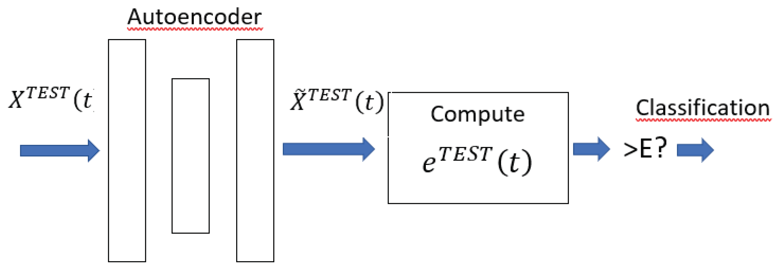
The classification is made by comparing the error with the threshold E in Equation (10) as indicated in Equation (15)
To summarize, the classifier is therefore built in two phases. During the training phase (Figure 1) the autoencoder learns to reconstruct vectors representing the normal behavior in an optimal way by setting the parameters of the neural network. This operation is done in this paper through a gradient descent, an iterative learning algorithm that uses several hyperparameters to update a model. At each iteration the model should be improved by updating the internal model parameters. Two hyperparameters that will be used in the performance evaluation are the batch size and number of epochs. The batch size controls the number of training samples (i.e., the number of rows in the matrix ) to use before the model’s internal parameters are updated. In practice, after the end of the batch, the input is compared with the output and the error is computed. Starting from the error the update algorithm is used to move down along the error gradient. The training dataset can be divided into one or more batches and this number is one parameter affecting the system performance analyzed in the Results section. The number of epochs defines the number of times that the learning algorithm will use the entire training dataset. An epoch is composed of one or more batches. The number of epochs should be large enough so that the learning algorithm can run until the error has been sufficiently minimized. The number of epochs is the second hyperparameter studied in the Results. After the training phase, a threshold E is set.
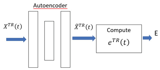
Figure 1.
Training phase.
In the test phase (Figure 2) the state vectors are sent to the autoencoder, and the reconstruction error is used to classify vectors.
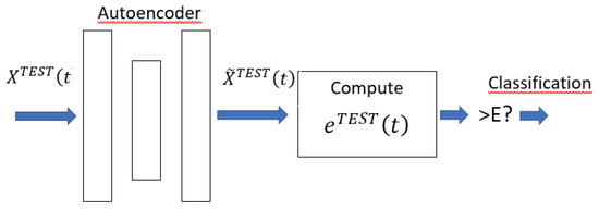
Figure 2.
Test phase.
4. Materials and Methods
The use case of this paper is a typical small-scale photovoltaic system connected to the grid at the distribution level. From an electrical point of view it is composed of solar panels, a DC-DC boost electronic converter controlled by the maximum power point tracking algorithm, a DC link and a current source inverter. The inverter acts also as a server sending information to and receiving commands from a control unit, which can be represented by a SCADA in the case of a microgrid or by a distribution management system in the case of distribution grid. The system is also equipped with different sensors that collect heterogeneous types of measurements. We categorize all the collectible information in five groups:
- Alternating Current (AC) side electrical information: active and reactive power, voltages (Root Mean Square, RMS), currents (RMS), frequencies, total harmonic distortion (THD)
- Direct-Current (DC) side electrical information: voltages and currents
- PV information: voltage, current, temperature of the cells
- Environmental information: irradiance, temperature of the air
- Electronic information: maximum power point, dc/dc converter duty cycle
As said, we would like to detect anomalies by the only observation of the collected measures. In order to validate the proposed approach, we set up a simulation environment. The physical behavior of the photovoltaic system is simulated by using MATLAB/Simulink software, as shown in Figure 3.

Figure 3.
Simulated environment on Simulink.
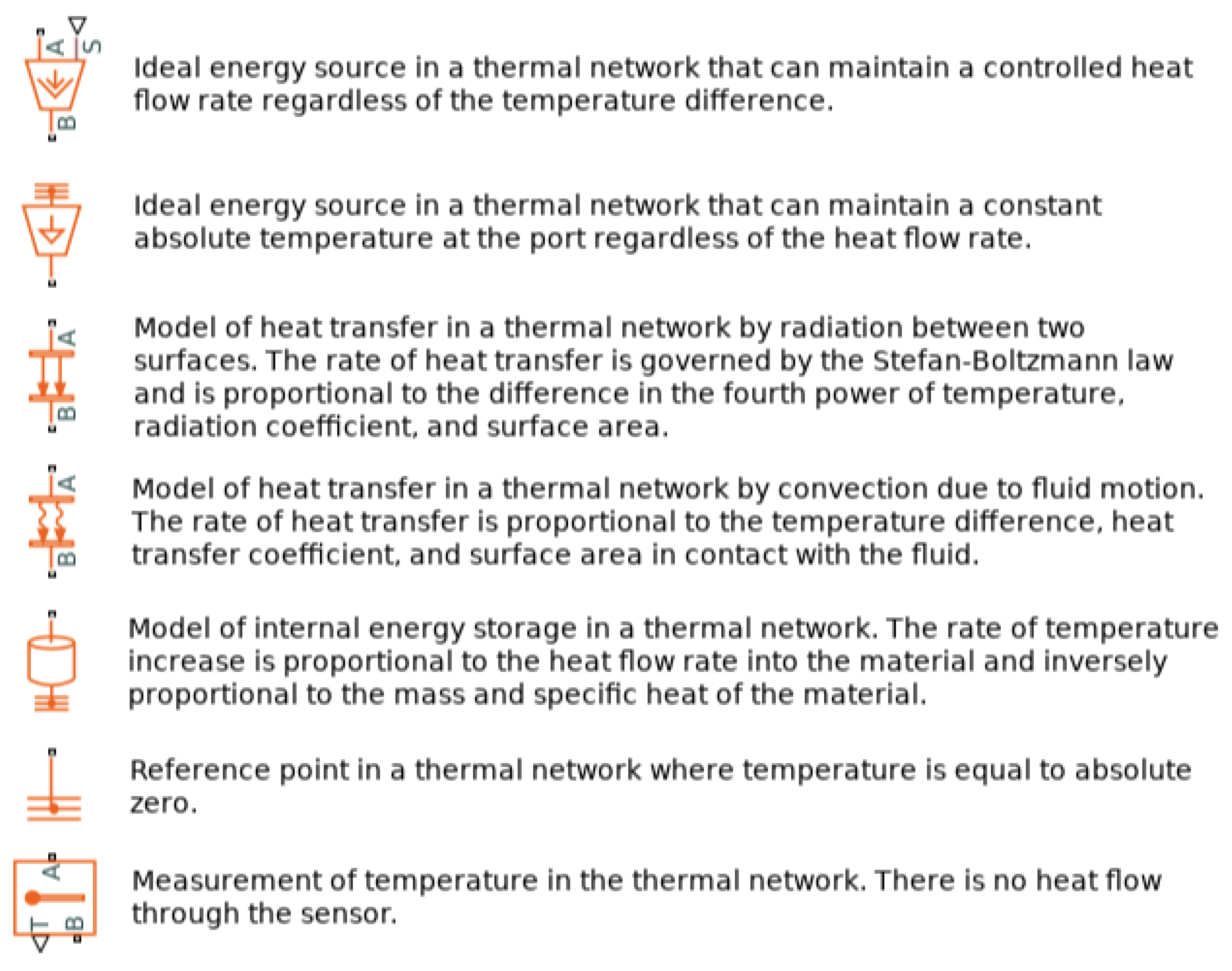
The scheme takes into account the heat exchange between the panels and the environment (in red in the left part of Figure 3) starting from the external data of solar irradiance and the temperature of the air. This is simulated by a radiation heat transfer coming from the sun, a convective heat exchange with the environment considered to be an ideal temperature source, and a thermal inertia of the photovoltaic panels. The legenda, taken directly in Simulink, concerning this part is reported in Figure 4.

Figure 4.
Legenda of thermal scheme.
Then we implemented an electromagnetic electrical model, the portion between the PV Array and the Inverter in Figure 3, starting from the blocks already present in the software. The grid is modeled by a small low voltage portion with some loads, and a transformer connected to the medium voltage distribution. We extract 22 features composing vector (1), which represent the physical parameters that are measured in many commercial solutions, especially in microgrids. The list of these features is reported in Table 1. The green boxes in Figure 3 are the points where we extract the measures listed in Table 1 from the system. Concerning the boxes that indicate the points where multiple measures are extracted: “PV_Meas” refers to and , i.e., and ; “AC measures” block is the point where we extract the measures from to . is measured within the MPPT converter. The model runs for different working conditions in order to create a large dataset.

Table 1.
List and description of the features.
We simulated three types of faults/cyber-attacks that have different impact on the measures:
- Reduction of active power injection
- Short circuit of some cells of the solar panel
- Bad data injection
In the first case, we use the remote-control capabilities of the inverter: the action implies a minor active power injection to the grid compared to the possible available power considering environmental conditions. In the second case, we consider a typical fault that can happen in a solar panel, which affects the performance of the panel itself. In the third case, we modify only one feature for sample, by changing its value of a percentage ranging from 25 to 50% of the original value, in order to create an unfeasible state vector. For instance, the injected power is modified maintaining unchanged voltage and current measures. A bad data injection attack can be dangerous for DERs because it can induce a wrong decision in a remote-control system.
The classification is performed offline on the test dataset. The autoencoder, implemented in Python by using Keras library [23], is a multilevel neural network (NN) architecture that uses input and output layers composed of the same number of neurons and a series of hidden layers whose dimension is strictly lower than the dimension of input and output layers. Neurons are fully connected, which means that each single neuron acts as an input for all the neurons of the following layer. The activation function of each neuron is a sigmoid. During the training phase, all the parameters of the neurons (i.e., the weights of the connections) are set by using the gradient descent technique. The impact on the performance of the following two hyperparameters, whose meaning is mentioned in Section 4, is evaluated in the following:
- Batch size
- Epochs
The variation of these hyperparameters can strongly influence the model learned by the NN.
5. Results
5.1. General Description
We extracted a training dataset composed of 7200 vectors, corresponding to about 30 days of operation under different weather conditions, and 3 test dataset composed of about 800 vectors corresponding to some hours of operation (because of a smaller sampling time with respect to the training set) in normal and abnormal conditions. Tests are made in order to evaluate the influence of different elements so to improve the efficiency of the detection method. We focused on the choice of the threshold E in Equation (10), on the neural network architecture, and on the hyperparameters used to train the NN.
5.2. Threshold E
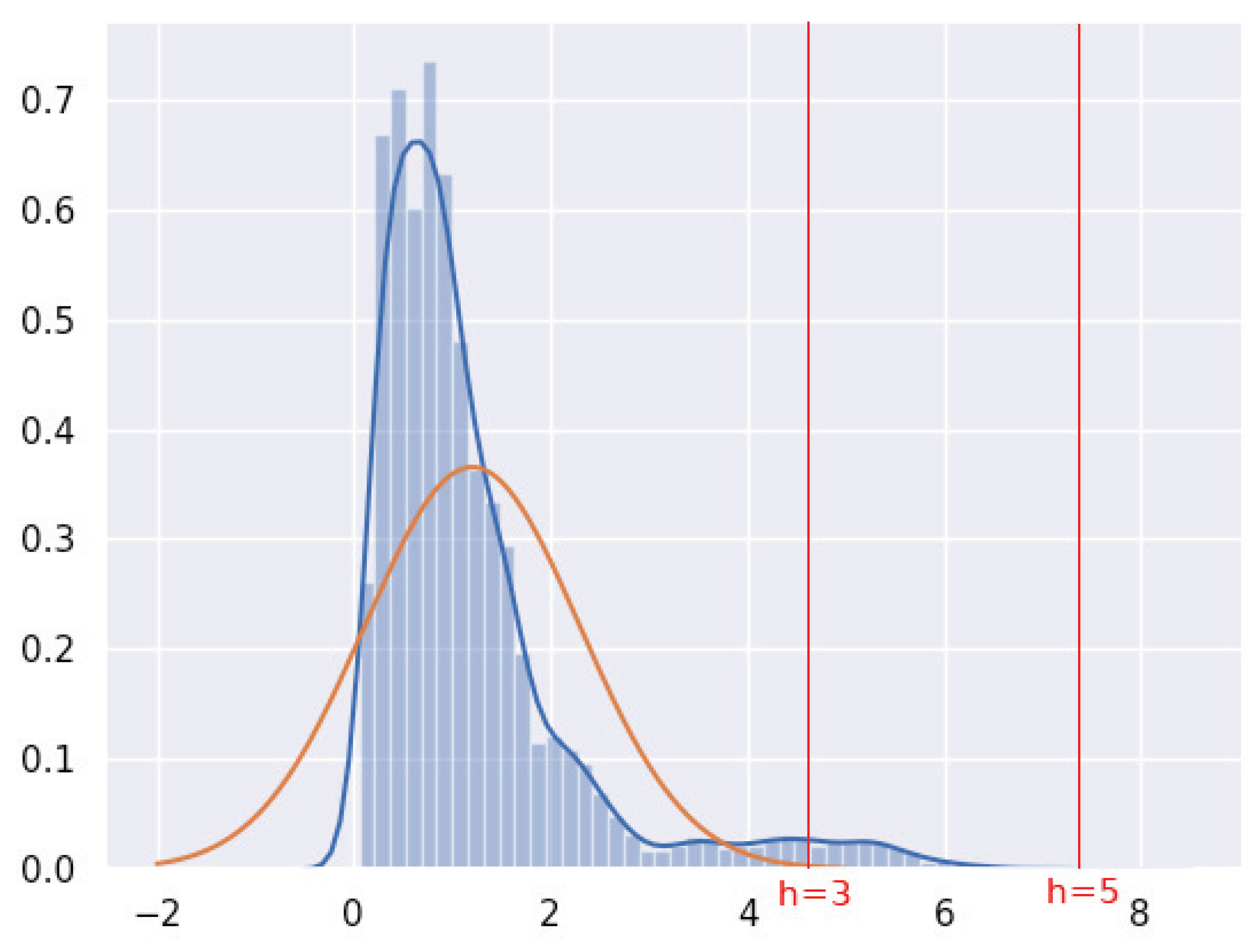
As indicated in Equation (10) we set the threshold E as the mean error plus h times the standard deviation of the error computed on the training dataset. As expressed in Section 4 the choice is theoretically fully justified if the probability density function of the error is Gaussian because, in this case, the area below the curve within the range identified by and is always equal to 0.6827, by and equal to 0.9545, by and equal to 0.9973, and so on, allowing h to control the probability that the random variable error is within the range defined by . Supposing that the distribution of is the same of the one of , h would allow the setting of a defined percentage of vectors as normal. Fixing the structure of the autoencoder with a single hidden layer of dimension 15, and low epochs (10) and high batch size (256), Figure 5 reports the histogram of the normalized errors, the curve that approximates the related probability density function, and the corresponding normal curve with the same mean and standard deviation (red line). The shapes are qualitatively similar by changing hidden layer dimension, epoch and batch size.
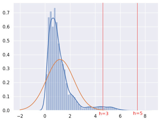
Figure 5.
Distribution of errors computed on training dataset.
We can notice that even if the distribution is different from the Gaussian, the proposed structure for the choice of the threshold may be still applied even if the selection of the h value must be heuristic. h can still select a percentage of vectors as normal, even if more coarsely than in the Gaussian case. In Figure 5 two values of the threshold are reported; the choice of has the intention to maintain a small number of false positives. To analyze numerically the effect on the performance we varied h from 3 to 7, as reported in Table 2. The motivation is that above and beyond results show that the performance decreases significantly. The acronyms TN, FN, FP and TP stand, respectively, for True and False Negative, and False and True Positive. Accuracy is the proportion of true results.

Table 2.
Impact of the choice of the threshold on accuracy.
These preliminary results highlight important aspects: the best threshold’s choice depends on the specific case because some physical anomalies produce higher errors that are more easily separable. For examples, anomalies that involve the modification of a high number of measures cause a higher reconstruction error. Therefore, setting a high value for the threshold E (through a higher h) reduces the number of false positives. On the contrary, anomalies that induce a small amount of measures to change cause a lower reconstruction error, consequently the threshold E should be maintained lower (through a lower h), even if this choice raises the number of false positives. If we want to avoid to loose generality, we must fix a threshold that is a compromise. On the first phase, we set .
5.3. Autoencoder Architecture
Subsequently, fixing , the impact of the NN architecture on the accuracy has been investigated. We tried different combinations of depth and number of neurons for hidden layer. For example, considering Table 3, “22-15-22” refers to an architecture composed of a single hidden layer whose dimension is 15 and an input and output layer each composed of 22 neurons corresponding to the number of features in Table 1, while “22-18-15-18-22" refers to an architecture composed of 3 hidden layers whose dimensions are 18, 15 and 18, respectively. The layers are fully connected, which means that each single neuron of a layer acts as an input for each neuron of the following layer.

Table 3.
Impact of the NN architecture on accuracy.
The number of neurons of the most compressed layer impacts on the accuracy more than the number of hidden layers. In the presented results, in some cases, the depth of the NN impacts negatively on the accuracy, but we can say, in general that the depth does not bring significant changes in the performance. A possible explanation is that the dimension of the smallest hidden layer is the element that mostly affects the reduced representation of the system and, consequently, the capability to learn the correlation between measures. If this dimension is too large, the autoencoder just reproduces its input; on the contrary, if the dimension is too small, the NN loses important information.
5.4. Training Parameters
Finally, we investigated the gradient descent’s hyperparameters, focusing on batch size and epochs. After the previous phases, we fixed the threshold to and the NN architecture to 22-18-15-18-22. We compared the results by using different learning hyperparameters. The first test focuses on the batch size, fixing the number of epochs to 10. Results are reported in Table 4

Table 4.
Impact of the batch size on accuracy.
The second test refers to the number of epochs. We fixed the batch size to 32 and we evaluated the impact on accuracy by varying the epochs (Table 5).

Table 5.
Impact of the epochs on accuracy.
There is a relevant impact of hyperparameters on the accuracy concerning anomalies caused by Short Circuited Cells and Bad Data Injection. More times the training samples are passed to the autoencoder during training phase, more accurate is the model fitted by the NN. The identification of anomalies that produces lower errors benefits from a more suitable model built around training samples.
6. Discussion and Future Research Issues
The previous chapter proposed a performance evaluation of the proposed algorithm to detect different anomalies. One of the main problem is to adapt the algorithm to perform well under different conditions. Setting specific parameters for each anomaly brings to significantly better results; however, if the algorithm can perform well with only specific anomalies, than it betrays its aim. The previous section allows getting a compromise. Concerning future research, it would be our intention to elaborate on the error distribution so finding out alternatives for the computation of the threshold E. A major investigation over the NN architecture can bring better results. This paper analyzed separately the impact of the threshold, of the architecture and of the gradient descent hyperparameters. Actually, these three elements are bounded: for example, the choice of the best threshold cannot be considered a totally separated problem with respect to the other two elements. In order to find a real optimal solution, we must consider all these elements at the same time. We could proceed by a brute-force strategy by trying all the possible combinations for discrete steps. Nevertheless, this would result in a huge amount of data. A better solution would be to implement a multi-parametric optimization during the design of the NN.
Many papers in the literature use supervised ML algorithms in order to detect anomalies. Supervised algorithms usually perform well in classification problems, but these methods cannot be exploited without disposing of labeled datasets. An idea may be comparing our approach with anomaly detection algorithms based on One-Class Support Vector Machine. A cyber-physical anomaly detection may be a complementary tool to traditional Intrusion Detection Systems that could be based on network traffic analysis. Many industrial protocols send measures on plain text to a centralized control system; an element that scans the network traffic and that can also perform a deep packet inspection could act together with the proposed scheme to detect possible anomalies.
7. Conclusions
The paper presents a novel approach to detect anomalies within a photovoltaic system connected to the grid. ML algorithms and in particular Deep Learning architectures may be fundamental tools for this kind of applications. The results show that the proposed method can be valid; still, further investigation has to be done to increase the efficiency and to generalize the proposal to different scenarios in DER application field.
Author Contributions
Conceptualization, G.B.G., M.M., M.R. and P.G.; methodology, G.B.G. and M.M.; software, G.B.G.; validation, G.B.G. and M.R.; formal analysis, G.B.G. and M.M.; investigation, G.B.G.; resources, M.M. and P.G.; data curation, G.B.G. and M.R.; writing–original draft preparation, G.B.G.; writing–review and editing, M.M.; visualization, G.B.G.; supervision, M.M.; project administration, M.M. and P.G.; funding acquisition, M.M. and P.G. All authors have read and agreed to the published version of the manuscript.
Funding
This research received no external funding.
Conflicts of Interest
The authors declare no conflict of interest.
Abbreviations
The following abbreviations are used in this manuscript:
| DER | Distributed Energy Resources |
| DL | Deep Learning |
| ICS | Industrial Control System |
| IDS | Intrusion Detection System |
| ML | Machine Learning |
| NN | Neural Network |
| RES | Renewable Energy Sources |
| SCADA | Supervisory Control and Data Acquisition |
References
- Chandola, V.; Arindam, B.; Vipin, K. Anomaly detection: A survey. ACM Comput. Surv. 2009, 41, 15. [Google Scholar] [CrossRef]
- Markou, M.; Sameer, S. Novelty detection: A review—Part 1: Statistical approaches. Signal Process. 2003, 83, 2481–2497. [Google Scholar] [CrossRef]
- Markou, M.; Sameer, S. Novelty detection: A Review—part 2: Neural network based approaches. Signal Process. 2003, 83, 2499–2521. [Google Scholar] [CrossRef]
- Amarbayasgalan, T.; Bilguun, J.; Keun, R. Unsupervised novelty detection using deep autoencoders with density based clustering. Appl. Sci. 2018, 8, 1468. [Google Scholar] [CrossRef]
- Chen, J.; Sathe, S.; Aggarwal, C.; Turaga, D. Outlier detection with autoencoder ensembles. In Proceedings of the SIAM International Conference on Data Mining, Houston, TX, USA, 27–29 April 2017; Society for Industrial and Applied Mathematics: Philadelphia, PA, USA, 2017. [Google Scholar]
- Chalapathy, R.; Aditya, K.M.; Sanjay, C. Anomaly detection using one-class neural networks. arXiv 2018, arXiv:1802.06360. [Google Scholar]
- Zhu, B.; Shankar, S. SCADA-specific intrusion detection/prevention systems: A survey and taxonomy. In Proceedings of the 1st Workshop on Secure Control Systems (SCS), Stockholm, Sweden, 12 April 2010; Volume 11. [Google Scholar]
- Radoglou-Grammatikis, P.I.; Panagiotis, G.S. Securing the smart grid: A comprehensive compilation of intrusion detection and prevention systems. IEEE Access 2019, 7, 46595–46620. [Google Scholar] [CrossRef]
- Xu, Y.; Yi, Y.; Tianran, L.; Jiaqi, J.; Qi, W.; Jiaqi, J.; Qi, W. Review on cyber vulnerabilities of communication protocols in industrial control systems. In Proceedings of the IEEE Conference on Energy Internet and Energy System Integration (EI2), Beijing, China, 26–28 November 2017. [Google Scholar]
- Gao, W.; Morris, T.; Reaves, B.; Richey, D. On SCADA control system command and response injection and intrusion detection. In Proceedings of the IEEE eCrime Researchers Summit, Dallas, TX, USA, 18–20 October 2010. [Google Scholar]
- Fovino, I.N.; Coletta, A.; Carcano, A.; Masera, M. Critical state-based filtering system for securing SCADA network protocols. IEEE Trans. Ind. Electron. 2011, 59, 3943–3950. [Google Scholar] [CrossRef]
- Zhao, J.; Gomez-Exposito, A.; Netto, M.; Mili, M.; Abur, A.; Terzija, V.; Kamwa, I.; Pal, B.; Singh, A.K.; Qi, J.; et al. Power system dynamic state estimation: Motivations, definitions, methodologies, and future work. IEEE Trans. Power Syst. 2019, 34, 3188–3198. [Google Scholar] [CrossRef]
- Hu, Q.; Fooladivanda, D.; Chang, Y.H.; Tomlin, C.J. Secure state estimation and control for cyber security of the nonlinear power systems. IEEE Trans. Control. Netw. Syst. 2017, 5, 1310–1321. [Google Scholar] [CrossRef]
- Li, Y.; Zhi, L.; Liang, C. Dynamic State Estimation of Generators Under Cyber Attacks. IEEE Access 2019, 7, 125253–125267. [Google Scholar] [CrossRef]
- Harrou, F.; Bilal, T.; Ying, S. Improved k NN-Based Monitoring Schemes for Detecting Faults in PV Systems. IEEE J. Photovolt. 2019, 9, 811–821. [Google Scholar] [CrossRef]
- Costamagna, P.; De Giorgi, A.; Magistri, L.; Moser, G.; Pellaco, L.; Trucco, A. A classification approach for model-based fault diagnosis in power generation systems based on solid oxide fuel cells. IEEE Trans. Energy Convers. 2015, 31, 676–687. [Google Scholar] [CrossRef]
- Kosek, A.M. Contextual anomaly detection for cyber-physical security in Smart Grids based on an artificial neural network model. In Proceedings of the IEEE Joint Workshop on Cyber-Physical Security and Resilience in Smart Grids (CPSR-SG), Vienna, Austria, 11–14 April 2016. [Google Scholar]
- Kosek, A.M.; Gehrke, O. Ensemble regression model-based anomaly detection for cyber-physical intrusion detection in smart grids. In Proceedings of the IEEE Electrical Power and Energy Conference (EPEC), Ottawa, ON, Canada, 12–14 October 2016. [Google Scholar]
- Principi, E.; Rossetti, D.; Squartini, S.; Piazza, F. Unsupervised electric motor fault detection by using deep autoencoders. IEEE/Caa J. Autom. Sin. 2019, 6, 441–451. [Google Scholar] [CrossRef]
- Pillai, D.S.; Blaabjerg, F.; Rajasekar, N. A comparative evaluation of advanced fault detection approaches for PV systems. IEEE J. Photovolt. 2019, 9, 513–527. [Google Scholar] [CrossRef]
- AbdulMawjood, K.; Shady, S.R.; Walid, G.M. Detection and prediction of faults in photovoltaic arrays: A review. In Proceedings of the IEEE 12th International Conference on Compatibility, Power Electronics and Power Engineering (CPE-POWERENG 2018), Doha, Qatar, 10–12 April 2018. [Google Scholar]
- Hornik, K.; Stinchcombe, M.; White, H. Multilayer feedforward networks are universal approximators. Neural Netw. 1989, 2, 359–366. [Google Scholar] [CrossRef]
- Chollet, F. Keras. 2015. Available online: https://keras.io (accessed on 28 February 2020).
Sample Availability: Samples of the compounds are available from the authors. |
© 2020 by the authors. Licensee MDPI, Basel, Switzerland. This article is an open access article distributed under the terms and conditions of the Creative Commons Attribution (CC BY) license (http://creativecommons.org/licenses/by/4.0/).


