Abstract
The paper addresses the problem of localization based on hybrid received signal strength (RSS) and time of arrival (TOA) measurements, in the presence of synchronization errors among all the nodes in a wireless network, and assuming all parameters are unknown. In most existing schemes, in fact, knowledge of the model parameters is postulated to reduce the high dimensionality of the cost functions involved in the position estimation process. However, such parameters depend on the operational wireless context, and change over time due to the presence of dynamic obstacles and other modification of the environment. Therefore, they should be adaptively estimated “on the field”, with a procedure that must be as simple as possible in order to suit multiple real-time re-calibrations, even in low-cost applications, without requiring human intervention. Unfortunately, the joint maximum likelihood (ML) position estimator for this problem does not admit a closed-form solution, and numerical optimization is practically unfeasible due to the large number of nuisance parameters. To circumvent such issues, a novel two-step algorithm with reduced complexity is proposed: A first calibration phase exploits nodes in known positions to estimate the unknown RSS and TOA model parameters; then, in a second localization step, an hybrid TOA/RSS range estimator is combined with an iterative least-squares procedure to finally estimate the unknown target position. The results show that the proposed hybrid TOA/RSS localization approach outperformed state-of-the-art competitors and, remarkably, achieved almost the same accuracy of the joint ML benchmark but with a significantly lower computational cost.
1. Introduction
Location estimation plays a key role in many applications, and is today attracting a great interest from both industry and academia. This process is sustained by the increasing widespread use of interconnected smart devices, which have the potential to enable seamless position capabilities at significantly reduced development costs. Indeed, besides the undisputed importance of the ultimate localization accuracy, the low-complexity requirement has been recently regarded as a fundamental need in most resource-constrained operational contexts, such as body area networks and wireless sensor networks (WSNs). In this respect, the design of localization solutions able to exploit the received radio frequency signals in an opportunistic way, without requiring any additional hardware, is of great practical interest.
Several approaches have been proposed in the literature to tackle the problem of node localization by leveraging information extracted from existing terrestrial technologies [1,2,3,4,5,6]. Among others, range-based solutions have been widely employed in popular terrestrial localization systems, especially in WSNs, where they are preferred to range-free techniques [7,8] thanks to their reduced complexity. Range information can be obtained by exploiting different characteristics of the received signals, namely received signal strength (RSS) [9,10,11,12,13,14,15,16], time (difference) of arrival (TOA/TDOA) [17,18,19,20], and angle of arrival (AOA) [21,22,23,24,25]. Hybrid approaches combining different types of measurements have also been proposed. For instance, references [26,27,28,29,30,31,32] investigated novel localization schemes based on the combined use of RSS and AOA measurements, which are able to achieve improved estimation performance. Although interesting, these techniques require enhanced hardware and processing capabilities that are usually not available on-board low-cost sensor nodes employed in typical WSN deployments; more precisely, AOA-based methods are not appealing in such contexts owing to the increased complexity and costs associated with multiple antennas.
TOA/RSS solutions better fit the requirements of low-cost contexts, thanks to their simplicity and ready availability, and the hybrid (joint) approach is interesting for its improved accuracy [33,34,35,36,37,38,39,40,41,42]. A theoretical study of the localization performance achievable using joint TOA/RSS measurements has been conducted in [33]. By providing the exact expression of the Cramér–Rao lower bound (CRLB), authors showed that such hybrid schemes can offer significant improvements in the estimation accuracy with respect to the case where RSS-only or TOA-only measurements are used. In [34], authors addressed the problem of target localization in presence of mixed line-of-sight (LOS)/non-line-of-sight (NLOS) scenarios. In a first step, the algorithm classifies all the links as either LOS or NLOS according to a parametric Nakagami distribution; then, the position is estimated through a weighted least squares (WLS) approach that considers the sole TOA measurements for those links identified as LOS and the RSS measurements for the NLOS paths. A novel algorithm to tackle the problem of target localization in adverse NLOS environments has been proposed in [35]. In this work, authors tried to mitigate the detrimental effects of NLOS biases on both RSS and TOA measurements by recasting the original (non-convex) problem as an approximated generalized trust region sub-problem. The ultimate target position estimate is then obtained by applying a bisection procedure based on an iterative squared range WLS approach. In [36], same authors addressed the more challenging scenario in which all paths are in NLOS. By assuming a partial knowledge of the NLOS biases affecting the collected measurements, the highly-dimensional localization problem can be approximated to a min-max problem in which the NLOS biases are treated as known nuisance parameters. Similarly to [35], the final target location is estimated by resorting to a robust bisection procedure within a generalized trust region framework.
It is worth noting that almost all the aforementioned localization schemes based on hybrid TOA/RSS measurements require that a partial or even perfect knowledge of the model parameters is available. Moreover, in most cases all the nodes in the network are implicitly assumed to be perfectly synchronized among each other. Although these assumptions are typically used to reduce the high dimensionality of the cost functions involved in the position estimation process, in practical WSN deployments, nodes are not synchronized to the same clock and all the model parameters are unknown, hence the need to be adaptively estimated “on the field”. Furthermore, in most operational scenarios, such as indoor environments and urban areas, the presence of dynamic obstacles (people, vehicles, etc.) introduces significant modifications in the surrounding environments, leading to channel characteristics that are non-stationary over time. Therefore, to address the problem of target localization in real applications, a preliminary calibration phase aimed at estimating the unknown channel parameters at run-time should be performed. On the one hand, such a procedure must be as simple as possible in order to suit multiple real-time re-calibrations even in low-cost applications; on the other hand, it must be fully automatic, that is, it should not require any external assistance, including human interventions and frequent configurations—for this reason, such a feature can be also called self-calibration.
In this paper, we address the problem of target localization based on the combined use of TOA and RSS measurements under the realistic case of self-calibrated parameters. This work is motivated by the analysis conducted in [43], where it is highlighted the biased nature of the distance estimates obtained via RSS-only ranging in case of self-calibrated channel parameters. The main objective of this paper is to investigate how a dynamic estimation of the TOA and RSS model parameters will impact the ultimate position estimation performance of joint TOA/RSS range-based localization. To this aim, we extended our previous work [44] by considering, in addition to the hybrid TOA/RSS range estimator proposed therein, a preliminary self-calibration stage and a final position estimation stage. In particular, differently from [44] where all the parameters are assumed to be known, in this paper, we consider the more realistic case where the model parameters are estimated “on the field” according to a self-calibration procedure (described in Section 3.1). Moreover, we explicitly address the problem of nodes synchronization by including the clock offsets in all the considered models, as opposed to [44], where nodes are assumed to be synchronized. Our results show that using estimated parameters in place of the ideal (true) ones introduces detrimental non-linear effects that cannot be easily mitigated, and may lead to localization errors that can be significantly bigger than those obtained assuming a perfect knowledge of the environment; nonetheless, the provided algorithm is able to perform the whole localization task in a real environment and in a fully automatic (unsupervised) way.
Summarizing, the paper provides a two-fold contribution. First, we formalize the hybrid TOA/RSS localization problem in presence of synchronization errors among all the nodes in the network, and derive the corresponding joint maximum likelihood (ML) estimator of target position and nuisance parameters. As we will see, such an estimator does not admit a closed form solution; moreover, due to the large number of nuisance parameters in the final cost function, a numerical optimization is practically unfeasible. To circumvent such issues, as a second contribution we design a novel two-step algorithm with reduced complexity to solve the joint TOA/RSS range-based localization problem; more specifically, we split the original problem into two separated phases:
- a first calibration phase carried out by the different nodes in the network to estimate all the unknown RSS and TOA model parameters, including the synchronization offsets;
- a second localization step that leverages the combination of hybrid TOA/RSS ranging and iterative least squares (ILS) approach to estimate the unknown target position.
It is worth highlighting that the proposed approach, in each of the two separated phases involved in the localization task, exploits cooperation between nodes with known positions (anchors) and the node to be localized (blind node). More precisely, anchors need to exchange their collected TOA/RSS measurements and to communicate the time instants they start to transmit to the blind node. In this respect, we assume that all nodes in the network are equipped with low-power radio technologies (e.g., based on IEEE 802.15.4 standard, such as ZigBee, 6LoWPAN, etc.) that enable communications in a range of a few meters, while still preserving the required power efficiency.
The rest of the paper is organized as follows. In Section 2 we provide the problem formulation and discuss the resolution of the joint estimation problem using both TOA and RSS measurements. In Section 3 we derive in details the proposed two-step localization approach with self-calibration. Section 4 is devoted to the performance assessment of the proposed approach also in comparison to natural competitors. We conclude the paper in Section 5.
2. Hybrid TOA/RSS Localization: Formulation and Resolution Approaches
We consider, as a reference scenario, a WSN deployed over a given area with static anchor nodes located at known positions , , with denoting the transpose operator, and a static blind node (also called target) with unknown position . In the following, we assume that the target is properly equipped to extract both RSS and TOA information from the signals transmitted by the anchors. Moreover, we address the case in which the involved links are in LOS. It should be recognized that multipath and NLOS biases are main sources of errors that severely penalize the achievable localization performance, especially when operating in harsh environments, such as urban canyons or indoor areas. However, as we have seen in Section 1, most of the papers addressing this topic assume that a partial or even perfect knowledge of the TOA/RSS models parameters is available, so that nodes can quantify the detrimental effects of NLOS biases and try to mitigate them. Conversely, in this work, we steered our focus on the more realistic case of self-calibrated network, that is, the unknown model parameters are estimated adaptively “on the field”. We anticipate that, even under the “more simplistic” assumption of LOS propagation, the hybrid TOA/RSS localization problem is highly non-linear and does not admit a closed-form solution, due to the presence of a very large number of nuisance parameters. Despite the relevance of the considered setup, to the best of our knowledge no practical solutions to this problem are available in the literature. For this reason, in this paper, we address the LOS-only localization problem, leaving the extension to the more challenging case of NLOS propagation as a future work. Starting from the set of N received signals (one from each anchor), the main goal is to estimate the target unknown position based on RSS and TOA measurements, whose models are discussed in the following.
2.1. RSS Model
Let , with , denotes the average power (in dB) that the blind node measures based on the signal transmitted by the i-th anchor. According to the widely-used path loss model [45], each can be explicitly expressed as:
where is the Euclidean distance operator, denotes the path loss exponent regulating the slope of the decaying power law, and is the power at reference distance ; in the following, we assume m without loss of generality. As to , it represents the normally-distributed (in dB) shadowing term having zero-mean and variance . It is worth noticing that fast signal variations related to small-scale fading effects can be mitigated by averaging over time ([11,46,47], see also [48] for details concerning the computational aspects); hence, Equation (1) is a sufficiently general model to represent the average received power as only affected by the shadowing component (), as also demonstrated by the extensive experimental campaigns conducted in [45,49,50,51]. Following the above model, we have that:
where denotes the Gaussian probability density function (pdf) with mean and variance , and the shadowing variance (expressed in dB) does not depend on the range.
The parameters , and describing the statistical characterization of the RSS measurements typically depend on the specific environment at hand. A value of is commonly used to represent free space propagation, while is typical for most realistic outdoor and indoor scenarios. As we have seen in Section 1, most of the existing hybrid TOA/RSS estimators assume that such values are perfectly known a priori. Although this assumption is reasonable to carry out theoretical analyses aimed at understanding the fundamental behaviors and limits of the proposed techniques, in practical WSN deployments all the model parameters are unknown and must be estimated “on the field”.
2.2. TOA Model
For the purposes of this paper, we assume that anchors and blind nodes are not perfectly synchronized to the same clock, as is typical in real scenarios. More precisely, the TOA information measured by the blind node based on the signal transmitted by the i-th anchor can be modeled as:
with c denoting the speed of light, while and are the offsets of the i-th anchor and target clocks with respect to an ideal one, respectively. The additive term represents the TOA measurement error and is modeled as a zero-mean Gaussian random variable with variance , the latter reflecting the specific receiver precision [52]. It is worth noting that Equation (3) implicitly assumes the transmit time is known. We recall that the proposed approach exploits cooperation between anchors and blind nodes. Therefore, such an information can be actually provided to the blind node by the i-th transmitting anchor. Although the TOA Model (3) neglects the presence of multipath and the drift of the clocks, it is widely-adopted in different WSN applications and several experiments have shown that it is a reasonable approximation in many cases [40,41,42,52,53].
According to Model (3), it thus follows that:
As aforementioned, state-of-the-art approaches typically assume that the model parameters are known. In the specific case of the TOA Model (3), it is also customary to assume that all the nodes in the network are perfectly synchronized to the same clock, that is, the offsets and are often even set to zero.
2.3. Joint Maximum Likelihood Position Estimation
Let and denote the RSS and TOA observation vectors collected at the blind node exploiting the signals from the N anchors. For the sake of notation, we can arrange the set of unknown RSS model parameters as:
and, similarly, we can stack the unknown TOA parameters as:
Using Equation (2), (4), the joint TOA/RSS likelihood function can be written as:
where and denote the pdfs of the RSS and TOA measurements, respectively. It is worth noting that Equation (7) represents the actual likelihood under the assumption that both RSS and TOA information are measured from independent sources. Indeed, the experimental campaigns conducted in [52,53] clearly show that measurements extracted from the same signal are weakly correlated; hence, assuming independence in Equation (7) is not detrimental to generality.
2.4. Resolution Approaches
As it can be noticed, the function in Equation (9) is highly non-linear and does not admit a closed-form solution. Moreover, due to the large number of nuisance parameters, a direct minimization of Equation (9) would require an impracticable multidimensional numerical optimization. A possible workaround is to split the problem into two separated phases: (i) calibration and (ii) localization. Although suboptimal, this approach is more adequate to the limited computational capabilities of common resource-constrained WSN nodes; furthermore, we recall (see Section 1) that assuming and are known or can be determined once and for all is not reasonable in real operating scenarios due to possible macro-variations of the environments over time; therefore, an automatic self-calibration step at run-time must be provided.
More specifically, in the calibration phase, we exploit knowledge of the anchors positions and a set of anchor-to-anchor and anchor-to-blind measurements to estimate the unknown nuisance parameters, as will be explained in Section 3.1. Once estimates of the nuisance parameters are available from the calibration phase, the optimization problem in Equation (8) can be reduced to a problem of position-only estimation (localization phase). For the case at hand, however, still the latter task cannot be performed in closed-form. Therefore, one has to resort to a numerical optimization algorithm (e.g., gradient-based iteration) or to a two-dimensional grid search [54]. It should be noticed that both these approaches have some drawbacks. In particular, the first one suffers from the well-known problem of local minima and, depending on the choice of the initial point, wrong or even missing convergence may be experienced. The second one is computationally much more expensive, especially when the area of interest can be large and medium- to fine-grained resolutions are needed; thus, it is indeed not preferable for low-cost WSN nodes due to its super-linear (quadratic) complexity growth.
The simpler alternative of a range-based localization task is thus considered here, that is, we further split the localization problem into two separated steps: (ii-a) ranging and (ii-b) position estimation. In doing so, we can leverage the hybrid TOA/RSS range estimator derived in [44]—which is available in closed-form—to perform distance measurements between the blind node and each anchor node. Once the set of N distance estimates is available at the blind node, the ultimate position estimation task can be then accomplished by resorting to a multilateration approach based on the well-established ILS procedure. Differently from other numerical optimization routines, the ILS has received significant attention thanks to its ability to achieve convergence in a small number of iterations, and is indeed widespread adopted in all commercial global navigation satellite system (GNSS) receivers [55]. Moreover, compared to (linearized) multilateration based on pairwise subtraction of the range measurement equations, significantly greater accuracy is achieved without major increase in computational complexity [8]. Indeed, several optimized variants of ILS have also been proposed in literature, which make ILS amenable to practical implementation even on resource-constrained devices, such as low-cost WSN nodes [56,57]. Although the whole localization procedure is suboptimal with respect to the initial ML estimation problem in Equation (8), we will show that the achievable performance of the proposed algorithm can be very close to the ones obtained via a two-dimensional grid search.
3. Proposed Localization Algorithm with Self-Calibration
In this section, we explain the proposed two-step localization algorithm in details. We start by describing the calibration phase, which is performed by both anchors and blind nodes to estimate the unknown TOA/RSS channel parameters. Such estimates are then used in the localization phase in part to correct the synchronization errors affecting all the TOA measurements (anchor-to-anchor and anchor-to-blind), and in part to compute the N distances among the blind node and each anchor in the network. In this respect, it is important to observe that, differently from the case where both and are assumed to be known (deterministic), the accuracy of the range estimates will also depend on the uncertainty affecting the TOA/RSS parameter estimation. More precisely, and will influence the ultimate distance estimation in a twofold fashion: directly, in all the anchor-to-blind measurements, and indirectly through estimation of the models parameters. As formally demonstrated in [44] for the case of RSS-only ranging, this injects severe non-linear effects that can dramatically affect the achievable performance. In the final step, range estimates are then fed, together with a coarse estimate of the blind position obtained in the calibration phase, to the ILS procedure which provides the final position estimate . In Figure 1, we provide a block diagram illustrating the main steps of the proposed localization solution.
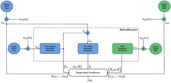
Figure 1.
Block diagram of the proposed hybrid time of arrival (TOA)/received signal strength (RSS) range-based localization with self-calibration.
3.1. TOA/RSS Parameters Estimation Using Self-Calibration
To formalize the calibration problem, we start by considering an abstract representation of the scenario at hand, as depicted in Figure 2.
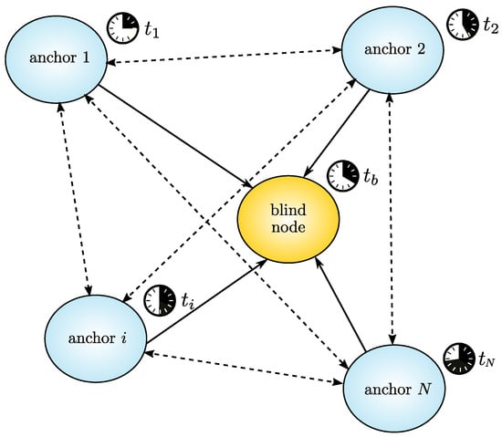
Figure 2.
A typical wireless sensor network (WSN) localization problem, with anchors and blind nodes not synchronized to the same clock. Dashed and solid arrows indicate anchor-to-anchor and anchor-to-blind measurements, respectively.
As it can be seen, there are different point-to-point communication links—either anchor-to-anchor or anchor-to-blind—from which both RSS and TOA measurements can be obtained. This general scenario can be representative of different operational environments (indoor or outdoor) as well as of different types of WSN applications (e.g., monitoring, rescue, etc.). As we have seen in Section 2, in practical WSN deployments not only the RSS and TOA model parameters are typically unknown, but they can also change over time owing to some macro-variation in the considered environment; therefore, an automatic procedure to estimate such parameters at run-time must be devised. To this aim, in the following we consider a self-calibration procedure that requires the sole knowledge of anchors’ positions, thus fulfilling the low-complexity requirements of conventional sensor networks [14,47,58].
In the first step of the calibration phase, we resort to the sole TOA anchor-to-anchor measurements in order to estimate the synchronization offsets , . According to the TOA model in Equation (3), we observe that the vector of measurements among the anchors can be written as:
with denoting the vector of the unknown clock offsets, and:
is a known vector. As to , it represents the vector of measurements errors defined as:
In the following, we assume that is a Gaussian random vector with and denoting the matrix of zeros and the K-dimensional identity matrix, respectively. Clearly, the set of measurements between anchors is independent from those received by the blind node, that is, is independent of the s. Moreover, the known matrix is given by:
and, as intuition might suggest, its role is practically to perform the time difference between the offsets of all anchor pairs. By posing , it follows that the likelihood function associated with the anchor-to-anchor TOA measurements can be expressed as:
It is a simple matter to show that the ML estimate of is given by:
where is the (orthogonal) projection matrix onto the orthogonal complement of the space spanned by the columns of . At this point, it should be noticed that the ML estimate of (namely the minimizer for in the previous formula) can be uniquely determined only when is a full-rank matrix. From the definition in Equation (13), it is not difficult to see that has rank ; therefore, we can estimate using a Least Squares (LS) approach as:
where , denotes the Moore-Penrose generalized inverse of , and represents the N-dimensional vector of ones.
The RSS model parameters can be estimated following the same procedure described in [14], where it is shown that ML estimation of the unknown vector reduces to a simple linear regression. More precisely, we start by observing that the vector of RSS measurements among the anchors can be written as:
where and denotes the vector of shadowing effects defined as:
Similarly to the TOA model, is a Gaussian random vector independent of the s. Moreover, we observe that is a known matrix with:
The likelihood function associated with the anchor-to-anchor RSS measurements can be expressed as:
As it can be noticed, Equation (20) has the same structure of the likelihood in Equation (14); hence, the ML estimate of can be easily computed by considering Equation (15) with and replaced by and , respectively. As to and , their final estimates (after some algebraic manipulations) are given by [14]:
where represents the sample mean of (i.e., ), denotes the sample variance of , and is the sample covariance between and . From these compact expressions, it follows that the ML estimate of can be obtained as:
The last step of the calibration phase involves the estimation of the blind node synchronization offset . To this aim, we start by considering the set of N anchor-to-blind TOA measurements, which we recall are given by:
At this point, it should be noticed that part of the synchronization errors in the above observations can be corrected by exploiting the estimates of the anchors offsets obtained through Equation (16). More precisely, we can define a new set of measurements:
where the synchronization errors due to the anchors clock offsets are assumed to be substantially compensated. In this respect, we remark that this approximation is only introduced at the design stage for the sake of mathematical tractability, while the actual algorithm performance will be evaluated in a realistic scenario which accounts for the residual effects of non-ideal calibrations. By multiplying both sides of Equation (25) by c, the following system of non-linear equations is obtained:
where denotes the pseudorange between the blind node and the i-th anchor estimated based on the TOA measurement , while represents the blind clock offset expressed in distance. In Equation (26), three equations are indeed sufficient to solve (in the least-squares sense) for the three unknowns and , but using more anchors () provides additional information that can lead in turn to better accuracy. To efficiently solve this (over-determined) non-linear system, an ILS procedure can be employed. The basic idea behind this approach consists in iteratively updating the estimates of the unknowns parameters and ; more precisely, we first differentiate the (noise-free versions of the) pseudorange. The term pseudorange is usually adopted in the range-based localization literature by analogy with the global positioning system (GPS) system, where range estimates can be obtained up to the synchronization offset between the (synchronous) satellite constellation and the user receiver, which in fact leads to the same problem as in Equation (26).
Calculations in Equation (26) obtain the system:
where , , and are treated as known and set equal to the current guess, and denotes the pseudorange resulting from the current guess of the unknown parameters, while the increments , and are considered as the sole unknowns. The new system in Equation (27) can then be solved by resorting to a LS approach:
where the obtained solutions are used to update the estimates of the sought parameters and . More precisely, the algorithm computes the difference between the pseudoranges calculated on the basis of the new guesses and the estimated ; then, is set as the new for the next iteration. An error metric is evaluated from the absolute values of , and , namely . The algorithm stops when is lower than a predefined threshold or when a maximum number of allowed iterations has been reached. The ILS algorithm is widely-used in commercial GNSS receivers (e.g., GPS) to retrieve the user position from a set of pseudoranges measured with respect to all the visible satellites. Remarkably, such an iterative procedure is robust against the problem of local minima and is able to achieve fast convergence (usually, less than 10 iterations are required).
It should be noticed that the outcomes of this last calibration step include, in addition to the estimated blind clock offset , also an estimate of the unknown blind position . However, we do not consider the latter as the ultimate estimate since it has been computed on the basis of the sole TOA information, which is known to provide very poor localization performance in some operational scenarios, in particular at short distances and for narrowband signals (and in fact motivates research on hybrid positioning). Therefore, in the following we will consider as a coarse initial estimate that will be used only to initialize a different ILS procedure employed in the final localization step, as described in the next section.
3.2. Hybrid TOA/RSS Range-Based Localization
In this section, we propose a two-step localization algorithm based on hybrid TOA/RSS range measurements between the blind node and all the anchors in the network. We first address the problem of range estimation by resorting to an adaptive variant of the hybrid estimator derived in [44]. Differently from such a previous work, in which all the parameters are assumed to be known, in this paper we consider the more realistic case where the model parameters have been estimated “on the field” according to the self-calibration procedure described in Section 3.1. Moreover, we explicitly address the problem of nodes synchronization by including the clock offsets in all the considered models, as opposed to [44] where nodes are assumed to be perfectly synchronized.
To formalize the hybrid range estimation problem, we recast the ML formulation in Equation (8) as a function of the sole unknown distances , , i.e.,
with an equivalent transformation of the negative log-likelihood, i.e.,
where we replaced the unknown TOA/RSS model parameters with their estimates obtained in the preliminary calibration phase. The hybrid TOA/RSS ML estimator is then obtained by imposing the first-order optimality condition:
which yields:
where we introduced to simplify the notation. Similarly to Equation (9), Equation (32) still does not admit any closed-form solution in . We can re-arrange Equation (32) as:
where . It can be noticed that the right-hand side of the above equation is quadratic in the unknown . Following the same idea of [44], we relax such a quadratic function to an affine function of the form , with m and q unknown parameters to be determined from a simple linear regression. Denoting with and the optimal (in the ordinary LS sense) values resulting from the linear fitting, it follows that Equation (33) reduces to:
Based on the above relaxation, the closed-form expression of the hybrid TOA/RSS range estimator for is given by:
where denotes the principal branch of the Lambert W-function [59] and, in turn,
with and , where A and B are design parameters representing the extrema of the interval used for the linear regression. The expression of the hybrid estimator for the case of requires only minor modifications; for the sake of conciseness, we omit it here and refer the interested reader to [44] for further details.
A few comments are now in order. First, we observe that the estimator provided in Equation (34) is only a function of the edges of the interval , which are thus two design parameters that can regulate the algorithm performance. Second, it is interesting to notice that grows as slow as ; therefore, the Lambert W-function can be efficiently computed by resorting to a look-up table that stores its values only in correspondence of integer arguments, without any appreciable difference in the obtained results. This nice property makes the hybrid estimator amenable to practical implementation even on low-cost nodes where only few kilobytes of memory are available for storage of local data.
The final positioning step will be performed by exploiting the N distance estimates , obtained by the blind node during the previous ranging phase. More precisely, we can set up the following system of nonlinear equations:
where denotes the generic error associated to the range estimation process. As it can be noticed, all the equations in Model (37) depend on the sole unknown blind position . To solve such a system, we consider a simpler variant of the ILS procedure applied to Equation (26), but without offsets in the range equations. In particular, we first differentiate the range equations to obtain the linearized system:
where and are regarded as the sole unknowns, while now we set the initial guess for and equal to the coarse estimate as obtained in the last step of the calibration phase. The LS solution of Equation (37) can be then computed as:
and is used to update the current estimate . In this case, the algorithm computes the difference between the estimated ranges and the predicted ranges calculated on the basis of the current guess . Then, is set equal to for the next iteration. Again, the algorithm stops when the error falls below a predefined threshold or when a maximum number of iterations has been exceeded.
As already discussed above, the ILS algorithm is robust against local minima and exhibits fast convergence. In other words, it can be considered a valid alternative to optimization routines (unfeasible for problem in Equation (8)) and, at the same time, a much lighter solution compared to a two-dimensional grid search.
4. Performance Assessment
In this section, we evaluate the performance of the proposed algorithm by means of Monte Carlo simulations. We consider, as a reference scenario, a WSN deployed over an area of m; in particular, the N anchors are distributed in the space so as to provide a good coverage in terms of connectivity, while the blind node is randomly located within the considered area and its position varies in each simulation trial. We consider for the RSS measurements the parameter = −30 dB, while for the path-loss exponent the two cases and are evaluated. As to the synchronization offsets s and , they are generated according to a uniform distribution in the interval where m and m represent the equivalent offsets expressed in terms of distances, respectively. In this analysis, we assume without loss of generality that both RSS and TOA measurements have the same accuracy, i.e., . Thus, all measurements have the same variance , i.e., neither measurement has better “quality” than the other. This is not always the case, of course, but this choice has the advantage of reducing the parameter space for the simulations to the most interesting case: in fact, in [44] it is shown that if TOA and RSS variances are (significantly) different, then one of the two sources of information always dominates; hence, the hybrid estimator boils down to the TOA-only or RSS-only estimator, accordingly. For the assessment we consider values of ranging from 3 to 6, which are representative of several operational scenarios of WSNs, from outdoor open spaces to propagation environments full of obstructions (e.g., people, furniture, …).
The proposed hybrid estimator is computed using and as in [44], and it is compared against the most natural competitor algorithms based on Newton–Raphson iterations, given in [53] and in the following labeled as NR1 and NR2. The basic difference among the NR1 and NR2 methods consists in the number of Newton–Raphson iterations performed to compute the distance estimate. More precisely, the NR1 algorithm uses a single iteration, while the NR2 algorithm employs two iterations. Even though such algorithms were originally designed for range estimation, the ultimate blind node position can be easily retrieved by resorting to the ILS procedure in Equation (39) based on the N distance estimates obtained during the ranging phase. For comparison purposes, we also report the performance of the (range-free) joint ML position estimator in Equation (8), obtained via a two-dimensional grid search. We, however, remark that the latter cannot be taken as a direct competitor since it is not available in closed-form; hence, it will be considered only as a benchmark. Moreover, we also compare the performance of the hybrid estimators against the more traditional algorithms based only on RSS or TOA information, denoted by “RSS-only” and “TOA-only”, respectively. To assess the ultimate algorithms performance, we consider the mean square error (MSE) metric, computed from the position error based on 1000 trials.
We start the analysis by investigating the computational complexity of all the considered approaches. More specifically, we have recorded the runtimes of the estimators executed on the same hardware platform, for a network with anchors. A grid of evaluation points per dimension is considered for the joint ML estimator. A comparison between the average runtimes of the different estimators (normalized to the fastest one, that is the NR-based method,) is provided in Figure 3.
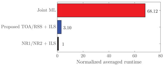
Figure 3.
Averaged runtimes of the considered localization approaches.
As expected, the joint ML requires by far the longest runtime due to the two-dimensional search involved in the solution of Equation (8). Remarkably, the proposed hybrid TOA/RSS approach has only slightly higher complexity compared to NR, while it is significantly less complex than the optimal joint ML.
In Figure 4, we report the MSEs of all the considered algorithms as function of the measurement error for and . The solid curves represent the ideal estimation performance obtained by assuming that the TOA/RSS model parameters and are perfectly known a priori, while the dashed curves show the corresponding versions with the unknown parameters replaced by their estimates obtained from the preliminary calibration phase presented in Section 3.1. The obtained results clearly show that the proposed hybrid estimator outperforms the state-of-the-art competitors for all the considered range of and, remarkably, can achieve almost the same accuracy of the joint ML benchmark, but at a significantly reduced computational cost. To better highlight the obtained results, in Figure 5 we depict the considered network with anchors for a given position of the target, together with a graphical representation of the estimated circular error probable (CEP) (the CEP is usually defined as the radius of the circle, centered in the average estimated position, which is expected to include 50% of the estimated positions) resulting from the application of the proposed hybrid TOA/RSS approach for the two specific cases of and .
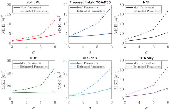
Figure 4.
Mean square error (MSEs) of the considered estimators as function of the measurement error for and : ideal vs. estimated parameters.
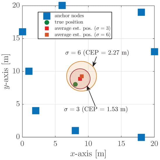
Figure 5.
Graphical representation of the considered network for and for a fixed target position. Shaded circles represent the circular error probable (CEP) of the proposed two-step localization approach for .
As expected, the actual performance in the more realistic case of self-calibrated algorithms are much worse compared to that obtained under ideal knowledge of the models parameters, especially for high values of . To corroborate such results, we investigate the performance of the self-calibration procedure adopted to estimate the unknown TOA/RSS model parameters. In Figure 6, we depict the estimation errors obtained during the calibration phase for the two values of the measurement error , which are representative of a “low-noise” and “high-noise” scenarios, respectively.
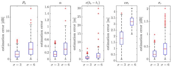
Figure 6.
Estimation errors obtained during the calibration phase for with and .
The obtained performance is in agreement with the findings in [43] (which however addressed the specific problem of RSS-only ranging): in fact, higher values of amplify the errors in the model parameters estimation and, in turn, introduce severe non-linear effects that are detrimental to the final positioning task. From this analysis, it clearly emerges that in practical WSN deployments—where the true values of the environmental parameters are unknown—the ultimate localization accuracy is also affected by the quality of the parameter estimation task.
To further investigate how a realistic calibration affects the localization process, in Figure 7 we report the algorithms performance as a function of the number of anchors N, now for the case and . As it can be noticed, for a sufficient number of anchors N, almost all the algorithms exhibit a satisfactory localization accuracy, in spite of the presence of a quite high noise level . Interestingly, for the dashed-curves (estimated parameters) closely attain the ideal ones (known parameters). Again, the proposed hybrid TOA/RSS position estimator offers the best performance, with an MSE below 10 m for almost all the considered span of N. These results are reasonable since for higher values of N the increasing amount of information collected within the network enables a much more accurate estimation of the unknown models parameters (through the self-calibration procedure proposed in Section 3.1); conversely, as N decreases, the algorithms performance experience a rapid degradation until achieving unacceptable results for a number of anchors . In addition to a higher amount of information in the network (anchor-to-blind measurements scale linearly with N, anchor-to-anchor measurements scale quadratically with N), increasing the number of anchors N also leads to a better coverage of the considered area, resulting in turn into more favorable geometric conditions for the estimation of the unknown blind position. To quantify the impact of a better distribution of the anchors in the space, in Figure 8 we evaluate the horizontal dilution of precision (HDOP) for each different number of anchors N.
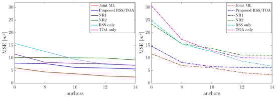
Figure 7.
MSEs of the considered algorithms as function of the number of anchors N for and . (left) Ideal TOA/RSS parameters and (right) estimated TOA/RSS parameters.
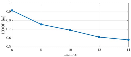
Figure 8.
Horizontal dilution of precision (HDOP) as function of the number of anchors N.
As it can be seen, increasing the density of anchors from 8 to 14 yields an accuracy improvement in terms of HDOP of about 40%.
As concerns the poor performance of the NR-based methods, it can be attributed to the fact that the hybrid TOA/RSS ranging problem is solved via a suboptimal approach based on Newton–Raphson iterations. More precisely, from the closed-form expressions of the estimators provided in [53], it can be noticed that the Newton–Raphson procedure is initialized with a coarse range estimate obtained using the sole TOA measurement; hence, it is reasonable to expect that the performance of both NR1 and NR2 approaches heavily depend on the accuracy of such data. Such theoretical considerations are in agreement with the performance of the NR1 method, whose performance curves are superimposed to the ones provided by the TOA-only estimator, hence are not visible in the figures, meaning that in the considered scenario one iteration of the Newton–Raphson method is indeed not sufficient to find a good approximate solution to the joint TOA/RSS ML problem.
To complete the analysis, in Figure 9 we show the empirical cumulative distribution functions (ECDFs) of the algorithms localization errors for the case , and assuming a number of anchors . As it can be noticed, a perfect knowledge of the models parameters would lead to positioning errors that are always below 7 m for all the hybrid estimators; conversely, in case of a realistic self-calibration, all the algorithms suffer evident impairments in the achieved performance, with errors that can even reach 20 m (tails of the ECDFs). Remarkably, the proposed hybrid estimator closely follows the joint ML benchmark, with a position error that is lower than 5 m in of the cases. As a confirmation, in Figure 10, we report the ECDFs of the localization errors for the challenging case of .
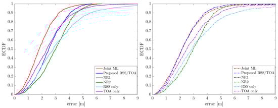
Figure 9.
Empirical cumulative distribution function (ECDF) of the considered algorithms for the case , and . (left) Ideal TOA/RSS parameters and (right) estimated TOA/RSS parameters.
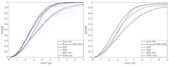
Figure 10.
ECDF of the considered algorithms for the case , and . (left) Ideal TOA/RSS parameters and (right) estimated TOA/RSS parameters.
As it could be expected, the obtained performance are generally worse than the ones in the previous case, especially for the RSS-only and TOA-only estimators which cannot mitigate the negative effects of an increased noise. Nevertheless, the proposed hybrid estimator still outperforms all the competitors, achieving localization performance that remains very close to the one provided by the joint ML. Notice also that for some percentile the joint ML has inferior performance; this is partially due to the fact that it is obtained by a numerical optimization of a non-linear function, which may not always terminate at the absolute maximum. Furthermore, in [44] it is shown that the hybrid TOA/RSS range estimator achieves a smaller MSE than the joint ML estimator (this is because of the bias-variance trade-off, i.e., it has been possible to design an estimator that is slightly biased but overall has a reduced value of MSE.); hence, this may, in turn, impact on the corresponding localization accuracy assessed here.
5. Conclusions
In this paper, we have addressed the TOA/RSS hybrid localization problem in presence of synchronization errors among all the nodes in the network and other missing information on the channel parameters. In fact, although many works assume knowledge of such parameters to reduce the high dimensionality of the cost functions involved in the position estimation task, such an information is not available in practice; moreover, parameters change over time due to the presence of dynamic obstacles and other modification of the environment; hence, automatic re-calibration is needed.
To circumvent the limitations of joint ML estimation—which is not available in closed-form and is practically unfeasible via numerical optimization due to the large number of nuisance parameters—we have designed a novel two-step algorithm with reduced complexity. In a first calibration phase, nodes in known positions are exploited to estimate the unknown RSS and TOA model parameters; then, in a second localization step, an hybrid TOA/RSS range estimator is combined with an iterative least-squares procedure to finally estimate the unknown target position. The results show that the proposed localization approach can outperform state-of-the-art competitors and, remarkably, achieve almost the same accuracy of the joint ML benchmark, but with significantly lower computational cost.
Author Contributions
All authors contributed equally to this work.
Funding
This research received no external funding.
Conflicts of Interest
The authors declare no conflict of interest.
References
- Gezici, S. A survey on wireless position estimation. Wirel. Pers. Commun. 2008, 44, 263–282. [Google Scholar] [CrossRef]
- Win, M.Z.; Conti, A.; Mazuelas, S.; Shen, Y.; Gifford, W.M.; Dardari, D.; Chiani, M. Network localization and navigation via cooperation. IEEE Commun. Mag. 2011, 49, 56–62. [Google Scholar] [CrossRef]
- Coluccia, A.; Fascista, A. A Review of Advanced Localization Techniques for Crowdsensing Wireless Sensor Networks. Sensors 2019, 19, 988. [Google Scholar] [CrossRef] [PubMed]
- Sayed, A.H.; Tarighat, A.; Khajehnouri, N. Network-based wireless location: Challenges faced in developing techniques for accurate wireless location information. IEEE Signal Process. Mag. 2005, 22, 24–40. [Google Scholar] [CrossRef]
- Dai, W.; Shen, Y.; Win, M.Z. Energy-efficient network navigation algorithms. IEEE J. Sel. Areas Commun. 2015, 33, 1418–1430. [Google Scholar] [CrossRef]
- Coluccia, A.; Ricciato, F.; Ricci, G. Positioning based on signals of opportunity. IEEE Commun. Lett. 2014, 18, 356–359. [Google Scholar] [CrossRef]
- Waadt, A.E.; Kocks, C.; Wang, S.; Bruck, G.H.; Jung, P. Maximum likelihood localization estimation based on received signal strength. In Proceedings of the 2010 3rd International Symposium on Applied Sciences in Biomedical and Communication Technologies (ISABEL), Rome, Italy, 7–10 November 2010; pp. 1–5. [Google Scholar]
- Coluccia, A.; Ricciato, F. RSS-based localization via Bayesian ranging and Iterative Least Squares positioning. IEEE Commun. Lett. 2014, 18, 873–876. [Google Scholar] [CrossRef]
- Tomic, S.; Beko, M.; Dinis, R. Distributed RSS-Based Localization in Wireless Sensor Networks Based on Second-Order Cone Programming. Sensors 2014, 14, 18410–18432. [Google Scholar] [CrossRef]
- Tomic, S.; Beko, M.; Dinis, R. RSS-based Localization in Wireless Sensor Networks Using Convex Relaxation: Noncooperative and Cooperative Schemes. IEEE Trans. Veh. Technol. 2015, 64, 2037–2050. [Google Scholar] [CrossRef]
- Patwari, N.; Hero, A.O., III; Perkins, M.; Correal, N.S.; O’Dea, R.J. Relative Location Estimation in Wireless Sensor Networks. IEEE Trans. Signal Proc. 2003, 51, 2137–2148. [Google Scholar] [CrossRef]
- Mao, G.; Fidan, B.; Anderson, B.D.O. Wireless Sensor Network Localization Techniques. Comput. Netw. 2007, 51, 2529–2553. [Google Scholar] [CrossRef]
- Wang, G.; Yang, K. A New Approach to Sensor Node Localization Using RSS Measurements in Wireless Sensor Networks. IEEE Trans. Wirel. Commun. 2011, 10, 1389–1395. [Google Scholar] [CrossRef]
- Coluccia, A.; Ricciato, F. On ML estimation for automatic RSS-based indoor localization. In Proceedings of the IEEE 5th International Symposium on Wireless Pervasive Computing, Modena, Italy, 5–7 May 2010. [Google Scholar]
- Salari, S.; Shahbazpanahi, S.; Ozdemir, K. Mobility-Aided Wireless Sensor Network Localization via Semidefinite Programming. IEEE Trans. Wirel. Commun. 2013, 12, 5966–5978. [Google Scholar] [CrossRef]
- Weiss, A.J. On the Accuracy of a Cellular Location System Based on RSS Measurements. IEEE Trans. Veh. Technol. 2003, 52, 1508–1518. [Google Scholar] [CrossRef]
- Wang, G.; Chen, H.; Li, Y.; Ansari, N. NLOS Error Mitigation for TOA-Based Localization via Convex Relaxation. IEEE Trans. Wirel. Commun. 2014, 13, 4119–4131. [Google Scholar] [CrossRef]
- Zhang, S.; Gao, S.; Wang, G.; Li, Y. Robust NLOS Error Mitigation Method for TOA-Based Localization via Second-Order Cone Relaxation. IEEE Commun. Lett. 2015, 19, 2210–2213. [Google Scholar] [CrossRef]
- Tomic, S.; Beko, M. Exact Robust Solution to TW-ToA-Based Target Localization Problem with Clock Imperfections. IEEE Signal Process. Lett. 2018, 25, 531–535. [Google Scholar] [CrossRef]
- Tomic, S.; Beko, M.; Dinis, R.; Montezuma, P. A Robust Bisection-Based Estimator for TOA-Based Target Localization in NLOS Environments. IEEE Commun. Lett. 2017, 21, 2488–2491. [Google Scholar] [CrossRef]
- Patwari, N.; Ash, J.; Kyperountas, S.; Hero, A.O., III; Moses, R.; Correal, N. Locating the nodes: Cooperative localization in wireless sensor networks. IEEE Signal Proc. Mag. 2005, 22, 54–69. [Google Scholar] [CrossRef]
- Rong, P.; Sichitiu, M.L. Angle of Arrival Localization for Wireless Sensor Networks. In Proceedings of the 3rd Annual IEEE Communications Society on Sensor and Ad Hoc Communications and Networks, Reston, VA, USA, 28 September 2006; pp. 374–382. [Google Scholar]
- Fascista, A.; Ciccarese, G.; Coluccia, A.; Ricci, G. A Localization Algorithm Based on V2I Communications and AOA Estimation. IEEE Signal Process. Lett. 2017, 24, 136–140. [Google Scholar] [CrossRef]
- Fascista, A.; Ciccarese, G.; Coluccia, A.; Ricci, G. Angle-of-Arrival based Cooperative Positioning for Smart Vehicles. IEEE Trans. Intell. Transp. Syst. 2018, 19, 2880–2892. [Google Scholar] [CrossRef]
- Fascista, A.; Ciccarese, G.; Coluccia, A.; Ricci, G. A change-detection approach to mobile node localization in bounded domains. In Proceedings of the 52nd IEEE Annual Conference on Information Sciences and Systems (CISS), Princeton, NJ, USA, 21–23 March 2018; pp. 1–6. [Google Scholar]
- Tomic, S.; Beko, M.; Dinis, R.; Montezuma, P. Distributed Algorithm for Target Localization in Wireless Sensor Networks Using RSS and AoA Measurements. Pervasive Mob. Comput. 2017, 37, 63–77. [Google Scholar] [CrossRef]
- Tomic, S.; Beko, M.; Dinis, R.; Montezuma, P. A Closed-form Solution for RSS/AoA Target Localization by Spherical Coordinates Conversion. IEEE Wirel. Commun. Lett. 2016, 5, 680–683. [Google Scholar] [CrossRef]
- Tomic, S.; Beko, M.; Dinis, R.; Gomes, J.P. Target Tracking with Sensor Navigation Using Coupled RSS and AoA Measurements. Sensors 2017, 17, 2690. [Google Scholar] [CrossRef]
- Tomic, S.; Beko, M.; Dinis, R. 3-D Target Localization in Wireless Sensor Networks Using RSS and AoA Measurements. IEEE Trans. Veh. Technol. 2017, 66, 3197–3210. [Google Scholar] [CrossRef]
- Tomic, S.; Beko, M.; Dinis, R.; Tuba, M.; Bacanin, N. Bayesian Methodology for Target Tracking Using RSS and AoA Measurements. Phys. Commun. 2017, 25, 158–166. [Google Scholar] [CrossRef]
- Tomic, S.; Beko, M.; Tuba, M. A Linear Estimator for Network Localization Using Integrated RSS and AOA Measurements. IEEE Signal Process. Lett. 2019, 26, 405–409. [Google Scholar] [CrossRef]
- Tomic, S.; Beko, M.; Dinis, R.; Bernardo, L. On Target Localization Using Combined RSS and AoA Measurements. Sensors 2018, 18, 1266. [Google Scholar] [CrossRef]
- Catovic, A.; Sahinoglu, Z. The Cramer-Rao Bounds of Hybrid TOA/RSS and TDOA/RSS Location Estimation Schemes. IEEE Commun. Lett. 2004, 8, 626–628. [Google Scholar] [CrossRef]
- Tiwari, S.; Wang, D.; Fattouche, M.; Ghannouchi, F. A Hybrid TOA/RSS Method for 3D Positioning in an Indoor Environment. ISRN Signal Proc. 2012, 2012. [Google Scholar] [CrossRef]
- Tomic, S.; Beko, M.; Tuba, M.; Correia, V.M.F. Target Localization in NLOS Environments Using RSS and TOA Measurements. IEEE Wirel. Commun. Lett. 2018, 7, 1062–1065. [Google Scholar] [CrossRef]
- Tomic, S.; Beko, M. A Robust NLOS Bias Mitigation Technique for RSS-TOA-Based Target Localization. IEEE Signal Process. Lett. 2019, 26, 64–68. [Google Scholar] [CrossRef]
- McGuire, M.; Plataniotis, K.N.; Venetsanopoulos, A.N. Data Fusion of Power and Time Measurements for Mobile Terminal Location. IEEE Trans. Mob. Comput. 2005, 4, 142–153. [Google Scholar] [CrossRef]
- Prieto, J.; Mazuelas, S.; Bahillo, A.; Fernández, P.; Lorenzo, R.M.; Abril, E.J. Adaptive Data Fusion for Wireless Localization in Harsh Environments. IEEE Trans. Signal Process. 2012, 60, 1585–1596. [Google Scholar] [CrossRef]
- Sahinoglu, Z.; Catovic, A. A Hybrid Location Estimation Scheme (H-LES) for Partially Synchronized Wireless Sensor Networks. In Proceedings of the 2004 IEEE International Conference on Communications (ICC), Paris, France, 20–24 June 2004. [Google Scholar]
- Bahillo, A.; Mazuelas, S.; Prieto, J.; Fernandez, P.; Lorenzo, R.M.; Abril, E.J. Hybrid RSS-RTT Localization Scheme for Wireless Networks. In Proceedings of the 2010 International Conference on Indoor Positioning and Indoor Navigation (IPIN), Zurich, Switzerland, 15–17 September 2010. [Google Scholar]
- Laaraiedh, M.; Avrillon, S.; Uguen, B. Hybrid Data Fusion Techniques for Localization in UWB Networks. In Proceedings of the 2009 6th Workshop on Positioning, Navigation and Communication (WPNC), Hannover, Germany, 19 March 2009. [Google Scholar]
- Laaraiedh, M.; Yu, L.; Avrillon, S.; Uguen, B. Comparison of Hybrid Localization Schemes using RSSI, TOA, and TDOA. In Proceedings of the 17th European Wireless 2011—Sustainable Wireless Technologies, Vienna, Austria, 27–29 April 2011. [Google Scholar]
- Coluccia, A. Reduced-Bias ML-Based Estimators with Low Complexity for Self-Calibrating RSS Ranging. IEEE Trans. Wirel. Commun. 2013, 12, 1220–1230. [Google Scholar] [CrossRef]
- Coluccia, A.; Fascista, A. On the Hybrid TOA/RSS Range Estimation in Wireless Sensor Networks. IEEE Trans. Wirel. Commun. 2018, 17, 361–371. [Google Scholar] [CrossRef]
- Rappaport, T.S. Wireless Communications: Principles and Practice, 2nd ed.; Prentice Hall: Upper Saddle River, NJ, USA, 2002. [Google Scholar]
- Zanca, G.; Zorzi, F.; Zanella, A.; Zorzi, M. Experimental comparison of RSSI-based localization algorithms for indoor wireless sensor networks. In Proceedings of the ACM Workshop on Real-World Wireless Sensor Networks, Glasgow, UK, 1 April 2008. [Google Scholar]
- Lim, H.; Kung, L.C.; Hou, J.C.; Luo, H. Zero-Configuration, Robust Indoor Localization: Theory and Experimentation. In Proceedings of the IEEE International Conference on Computer Communications, Barcelona, Spain, 23–29 April 2006. [Google Scholar]
- Coluccia, A.; Ricciato, F. A Software-Defined Radio tool for experimenting with RSS measurements in IEEE 802.15.4: Implementation and applications. In Proceedings of the 2012 21st International Conference on Computer Communications and Networks, Munich, Germany, 30 July–2 August 2013. [Google Scholar]
- Bernhardt, R.C. Macroscopic Diversity in Frequency Reuse Radio Systems. IEEE J. Sel. Areas Commun. 1987, 5, 862–870. [Google Scholar] [CrossRef]
- Babich, F.; Lombardi, G. Statistical Analysis and Characterization of the Indoor Propagation Channel. IEEE Trans. Commun. 2000, 48, 455–464. [Google Scholar] [CrossRef]
- Andersen, J.B.; Rappaport, T.S.; Yoshida, S. Propagation Measurements and Models for Wireless Communications Channels. IEEE Commun. Mag. 1995, 33, 42–49. [Google Scholar] [CrossRef]
- Macii, D.; Colombo, A.; Pivato, P.; Fontanelli, D. A Data Fusion Technique for Wireless Ranging Performance Improvement. IEEE Trans. Instrum. Meas. 2013, 62, 27–37. [Google Scholar] [CrossRef]
- Zhang, J.; Ding, L.; Wang, Y.; Hu, L. Measurement-based indoor NLoS ToA/RSS range error modelling. Electron. Lett. 2016, 52, 165–167. [Google Scholar] [CrossRef]
- Press, W.H.; Teukolsky, S.A.; Vetterling, W.T.; Flannery, B.P. Numerical Recipes: The Art of Scientific Computing, 3rd ed.; Cambridge University Press: Cambridge, UK, 2007. [Google Scholar]
- Tsui, J.B.-Y. Fundamentals of Global Positioning System Receivers: A Software Approach; Wiley: Hoboken, NJ, USA, 2000. [Google Scholar]
- He, Y.; Martin, R.; Bilgic, A.M. Approximate iterative Least Squares algorithms for GPS positioning. In Proceedings of the 10th IEEE International Symposium on Signal Processing and Information Technology, Luxor, Egypt, 15–18 December 2010; pp. 231–236. [Google Scholar]
- Yan, J.; Tiberius, C.C.J.M.; Teunissen, P.J.G.; Bellusci, G.; Janssen, G.J.M. A Framework for Low Complexity Least-Squares Localization with High Accuracy. IEEE Trans. Signal Process. 2010, 58, 4836–4847. [Google Scholar]
- Coluccia, A.; Ricciato, F. Maximum Likelihood trajectory estimation of a mobile node from RSS measurements. In Proceedings of the 9th Annual Conference on Wireless on-Demand Network Systems and Services (WONS), Courmayeur, Italy, 9–11 January 2012; pp. 151–158. [Google Scholar]
- Corless, R.M.; Gonnet, G.H.; Hare, D.E.G.; Jeffrey, D.J.; Knuth, D.E. On the Lambert W Function. Adv. Comput. Math. 1996, 5, 329–359. [Google Scholar] [CrossRef]


© 2019 by the authors. Licensee MDPI, Basel, Switzerland. This article is an open access article distributed under the terms and conditions of the Creative Commons Attribution (CC BY) license (http://creativecommons.org/licenses/by/4.0/).