Utilization of a Non-Linear Error Function in a Positioning Algorithm for Distance Measurement Systems Designed for Indoor Environments ^†

Abstract

A new positioning algorithm for distance measurement systems is outlined herein. This algorithm utilizes a non-linear error function which allows us to improve the positioning accuracy in highly difficult indoor environments. The non-linear error function also allows us to adjust the performance of the algorithm to the particular environmental conditions. The well-known positioning algorithms have limitations, mentioned by their authors, which make them unsuitable for positioning in an indoor environment. In this article, there is a brief discussion about the most popular positioning algorithms with consideration of the indoor environment. The new positioning algorithm is described in detail and a comparative performance analysis of the well-known algorithms and the proposed one is conducted. Those research results are achieved with the utilization of real distance measurement data, collected inside a few different buildings, and they show that the proposed algorithm outperforms the Chan and Foy algorithms in indoor environments. In this article the Automatic Person Localization System (SALOn) is also presented, which was utilized to collect measurement data.

1. Introduction

Interest in indoor positioning is continually growing. Good evidence of this statement is the InLocation Alliance, founded in 2012. At that time, 22 companies including Huawei, Samsung, and Broadcom joined the alliance to elaborate one indoor localization system and to find new business possibilities for indoor localization. Now the number of members is 34 and the group is working on accelerating the adoption of indoor positioning solutions to increase the mobile experience by opening up new opportunities [1]. There is already a great number of possible applications that utilize radio localization. The first to be mentioned are those applications that concern public safety. A good example of such a system is the Geospatial Location, Accountability, and Navigation System for Emergency Responders (GLANSER), developed to assist firefighters inside buildings in an emergency [2]. The SALOn system was developed for the same purpose at Gdansk University of Technology [3]. A building on fire is usually a death trap, not only for victims, but also for rescue teams. A person may be hit or overwhelmed by the collapsing structure. Additionally, situations of getting lost in an unknown building very often occur where there is a lack of visibility due to dense smoke. This is the reason why the localization system would improve the safety of firefighters and the effectiveness of rescue actions [4,5,6]. Other applications that address safety matters are those offered by the Guardly company, which combine indoor localization systems, the Global Positioning System (GPS), and solutions for suspicious activity report management to improve situational awareness that helps security operators monitor, manage, and respond to real data, leading to considerably shortened emergency response times [7]. Applications that automatically locate people who make emergency calls from their cellular phone are said to be the most important of the location services [8]. Another field in which radio localization is used is in care systems for elderly and disabled persons. The Warsaw University of Technology is one of the participants in the NITICS project, which stands for Networked Infrastructure for Innovative Home Care Solutions [9]. Continuous monitoring of an elderly person’s movements in their home allows for the detection of distressing symptoms and for an alarm to be sent to a family member or another attendant [10]. There are also applications connected with the commercial utilization of radio positioning, such as smart museums [11], and solutions to improve the making of business decisions by analyzing customers’ behavior [12,13], not to mention all kinds of sensor networks which make a particular environment a “smart” one.

The applications mentioned above are only a few possible utilizations of information about the positions of people and objects. Such information could also be used in factories, by logistic companies, and on construction sites. Despite the immense demand for information about position, indoor localization systems are still not as common as one may expect. This is caused by the occurrence of specific electromagnetic wave propagation conditions in such environments, which makes the utilization of well-known satellite navigation systems, such as GPS or Global Navigation Satellite System (GLONASS), very difficult or impossible. What is more, those conditions make the design of radio localization systems in such environments a complex process. The occurrence of reflection, deflection, and dispersion has a great impact on indoor radio wave propagation. That is why these factors must be taken into account while deploying reference stations for a radio localization system inside a building, as well as while choosing a proper positioning algorithm. 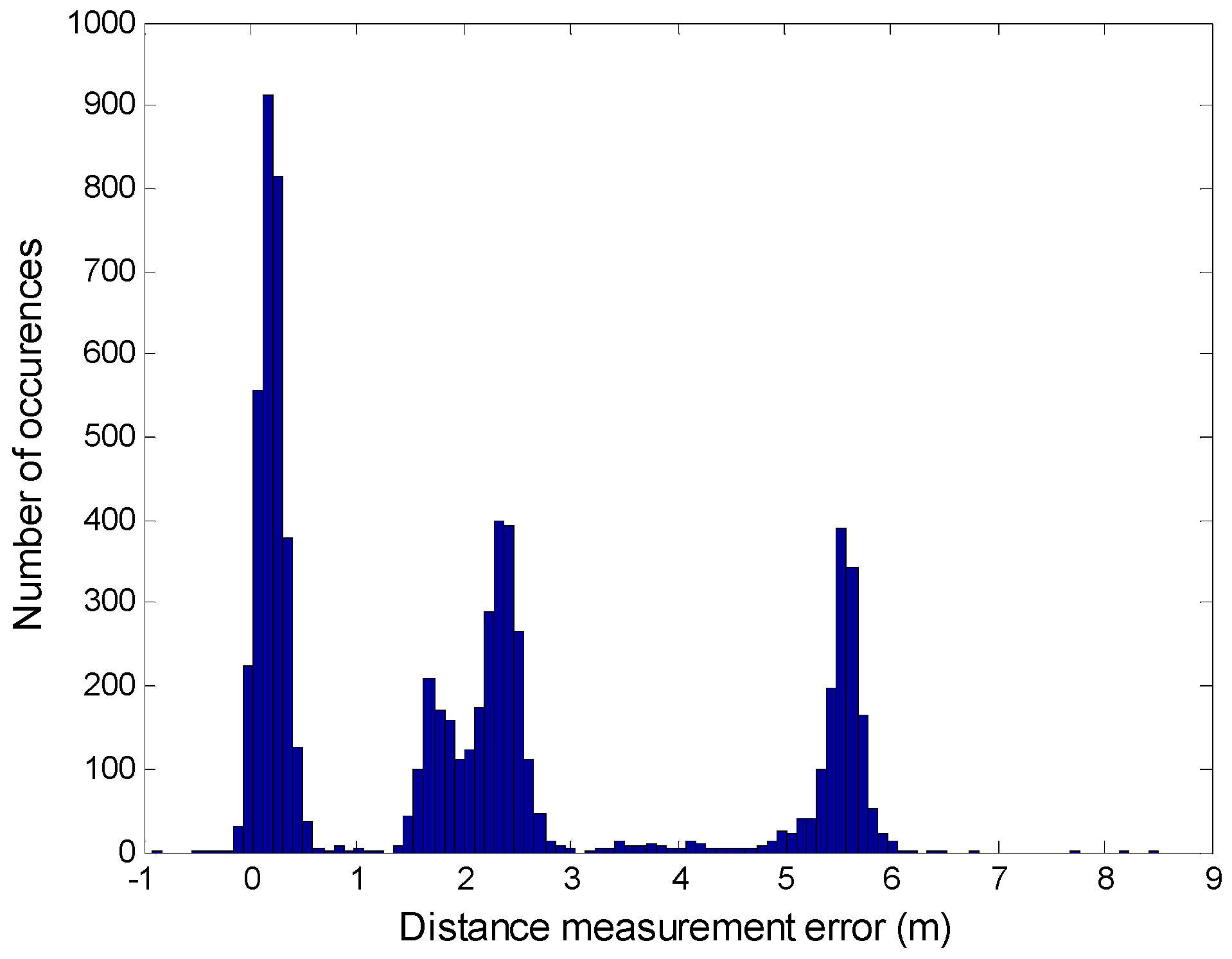For example, if a localization system utilizes TOA (Time of Arrival) or RTT [14] (Round Trip Time) methods, it most likely uses the Chan [15,16,17] or Foy [18,19,20] algorithm to calculate position. However, the authors of those algorithms remarked that the error distribution of input data should be Gaussian and the mean value of those errors should be equal to zero. Unfortunately, those conditions are usually not fulfilled in an indoor environment. This is because devices that realize distance measurements very often do not stay within the line of sight. They are separated by walls, furniture, or people. This leads to inflated distance measurements in comparison to the true distance between devices measured along the shortest route. As a consequence, the mean error of distance measurements is usually greater than zero. The mean values of distance measurement errors for different reference stations often vary. This makes the errors of input data for positioning algorithms follow a non-Gaussian distribution. An exemplary error distribution of real distance measurements conducted inside a single-family house is presented in Figure 1. It was plotted with the utilization of 7269 distance measurements made by one localized device. The mean error for this data is equal to 2.27 m. The influence of multipath propagation is clearly seen in the figure as there are several peaks for different values of distance measurement error.

Taking into consideration the above statements, there is a need to design a new positioning algorithm based on indoor radio distance measurements that would improve positioning accuracy by taking into account selected features of the radio wave propagation environment. The proposition of such an algorithm is presented in this article. There is also a brief description of two well-known positioning algorithms, as well as distance measurement methods. Additionally, the SALOn system, utilized to gather real radio distance measurements, is described. Those real distance measurements were utilized to conduct a comparative analysis of the proposed algorithm with the Chan and Foy algorithms. The presented results prove that the proposed algorithm outperforms the known positioning algorithms as far as an indoor environment is concerned.

The paper is structured as follows. In Section 2 there is a brief description of positioning based on radio distance measurements. In Section 3, the Chan and Foy algorithms are briefly discussed. In Section 4, the proposed new positioning algorithm is described in detail. In Section 5, the SALOn system is presented. Section 6 provides research results. Finally, Section 7 draws some conclusions.

2. Positioning Based on Distance Measurements

The distance between devices is measured indirectly by measurement of the propagation time. Knowing the propagation time, ${\tau }_i$, and the speed of the electromagnetic wave, $c$, one can calculate the distance to the $i$th reference station [22] by

$$R_i=c·{\tau }_i,i=1, 2,\dots , M,$$

(1)

where $M$ is the number of reference stations. If the coefficients of a reference station are $X_i$, $Y_i$ and the coefficients of a positioning object are $x$, $y$, then, for the two-dimensional case, the following equation may be written:

$$R_i=\sqrt{{\left(X_i-x\right)}^2+{\left(Y_i-y\right)}^2}.$$

(2)

This equation describes a circle, the center of which is determined by position of the reference station. The position of the localized object lies somewhere on the circle. To find the exact position of the localized object there must be at least three realized distance measurements (in the two-dimensional case). Then, all circles will cross in the object position. In the three-dimensional case, there is a need for at least four distance measurements, and Equation (2) must be transformed to a sphere formula. It is important that, in the two-dimensional case, reference stations must not be collinear and, in the three-dimensional case, they must not be coplanar. In both cases, reference stations must not move and their positions must be exactly known.

The basic distance measurement method is TOA, where distance measurements to all reference stations are made simultaneously. However, in this method there is a problem with time synchronization between all devices (reference stations and localized objects). Each device must be equipped with highly stable and expensive clocks. An alternative to TOA is the RTT method, where the distance measurement is realized as a measurement of radio signal propagation time in two directions of radio transmission [23]. Then, the device which sends the initial data package has the information about the starting time and ending time of the transmission. The difference between these times and the delay time of the reply multiplied by half of the speed of the electromagnetic wave is equal to the distance between these devices. In the literature, this method is also called two-way ranging (TWR) [24]. A method called symmetric double-sided two way ranging (SDS TWR) is also used. In this method, TWR measurements are realized twice, enabling them to decrease the influence of clock drift on distance measurements [25,26]. However, the RTT method is suitable only for slowly moving objects (like in an indoor environment) due to the non-simultaneous distance measurements to reference stations.

3. Selected Known Positioning Algorithms

To calculate position on the basis of distance measurements, the Chan or Foy algorithms are very often used.

The Chan algorithm was developed for hyperbolic systems where position calculation is based on time difference of arrival (TDOA). However, it can be also easily applied to distance measurement methods, as described in Reference [27]. The Chan algorithm is a non-iterative approach and is an approximate realization of the maximum likelihood method.

The Foy algorithm is an iterative one and uses an approximation of non-linear equations by the first two elements of their Taylor series. In distance measurement methods in two-dimensional cases, it is exploited to solve Equation (2).

The authors of both algorithms remarked that the error of the input data ought to have a Gaussian distribution with a mean value equal to zero. These conditions are not fulfilled in an indoor environment. Another disadvantage of these algorithms is the operation of matrix inversion utilized in both algorithms. This operation is not always possible due to mathematical reasons, which could be caused by a specific arrangement of reference stations or distance measurement errors. In consequence, it may happen that that algorithm will not allow us to obtain the position coordinates of the object.

4. The Proposed Positioning Algorithm for Distance Measurement Systems

The proposed new algorithm (already published in Reference [21]) is an iterative approach for position calculation in an indoor environment. It improves positioning accuracy compared to the Chan and Foy algorithms by taking into account selected features of the propagation environment. Moreover, in the proposed algorithm, matrix inversion is omitted, so it always returns a position, in contrast to the Chan and Foy algorithms.

The proposed algorithm is, in some aspects, similar to gradient algorithms. In such algorithms the direction of the greatest descent is searched on the basis of the gradient value, calculated for the function whose minimum we are looking for [28]. However, in the proposed algorithm, the gradient of a function is not calculated. Instead, in every iteration, coordinate correction values are calculated and added to the coordinates determined in the previous iteration. These correction values are proportional to some non-linear function (which will be referred to as a non-linear error function) normalized by the difference between the estimated proper coordinate of the localized object and the known proper coordinate of the reference station, divided by the estimated distance from the localized object to the reference station. This non-linear error function is the most important part of the proposed algorithm as it allows us to consider the environmental conditions and calibrate the algorithm.

To calculate the position coordinates, the following procedures must be accomplished in every iteration. The estimated distance from the localized object to each reference station (there is a need of at least three reference stations in a two-dimensional case) must be calculated using

$$r_i=\sqrt{{\left(X_i-x_v\right)}^2+{\left(Y_i-y_v\right)}^2},$$

(3)

where $r_i$ is the estimated distance to the ith reference station, $X_i$, $Y_i$ are coordinates of the ith reference station, and $x_v, y_v$ are the estimated coordinates.

Next, the coordinate correction values must be determined for every distance measurement done in the particular moment, as follows:

$$\begin{array}{c}\Delta X_i=\alpha ·f\left(R_i,r_i\right)·\frac{x_v-X_i}{r_i},\\ \Delta Y_i=\alpha ·f\left(R_i,r_i\right)·\frac{y_v-Y_i}{r_i},\end{array}$$

(4)

where $\alpha$ is a constant, which has an impact on algorithm convergence and stability (This parameter is similar to the step size or learning rate [29] used in gradient descent algorithms); $R_i$ is the distance measurement to the $i$th reference station, and $f\left(R_i,r_i\right)$ is the non-linear error function defined by Formula (7).

The constant $\alpha$ is set once for the particular measurement equipment. A calibration must be performed with the utilization of the real distance measurements in different environments. Such a calibration was performed on the basis of distance measurements realized in three environments, as follows: When all devices were placed in open space, when all were placed inside a building, and when anchors were outside the building while the localized object was inside. This research allowed us to tell that when $\alpha$ was too big (greater than 0.3 for all cases) the algorithm was not convergent; the values of the coefficient corrections (Equation (6)) did not reach a threshold. If $\alpha$ was equal to or lower than 0.2, the algorithm was always convergent. However, for smaller values of $\alpha$, the mean number of iterations was greater. Finally, for the SALOn system, $\alpha$ was set to 0.2.

After every iteration, new position coordinates are calculated, as follows:

$$x_{vN}=x_v+\Delta X_c,y_{vN}=y_v+\Delta Y_c,$$

(5)

where

$$\Delta X_c=\frac{1}{M}{{\displaystyle \sum }}_{i=1}^M\Delta X_i,\Delta Y_c=\frac{1}{M}{{\displaystyle \sum }}_{i=1}^M\Delta Y_i,$$

(6)

and $M$ is the number of reference stations taking part in measurements in the particular moment.

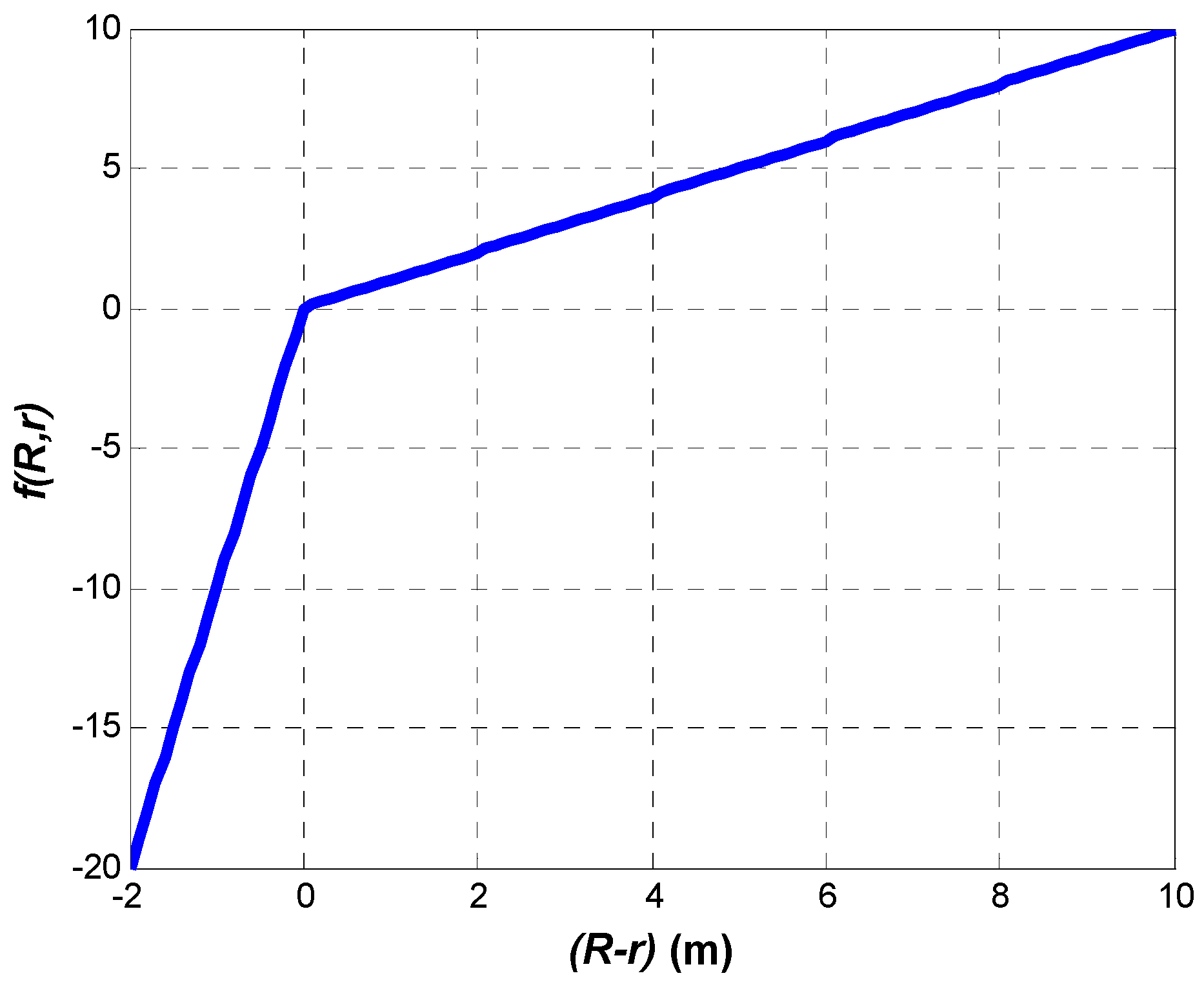
The most important element of the proposed algorithm is the non-linear error function, as it takes into account the propagation conditions of the environment. The distance measurements in an indoor environment are, in most cases, greater than the real ones, due to the multipath propagation. The radio signal is propagated, usually not along the shortest path but a longer one. In consequence, the measured propagation time is greater than that which would result from the true distance between devices. Thus, it may be assumed that the estimated distance should be lesser than the measured one. This is the reason why the coordinate correction values ought to be small when the estimated distance is smaller than the measured one. However, when the estimated distance is bigger than the measured one, the coordinate correction values should be considerable, as in such a case there is a great probability that the coordinates of the localized object are estimated with a huge error. The above considerations allowed us to heuristically select the shape of the non-linear error function. It must be said that this shape has changed over the last five years [21]. The presented non-linear error function was chosen as it makes the algorithm convergent and stable and it gives the best position estimation accuracy from the considered shapes of that function. The final non-linear error function is defined as follows:

$$f\left(R,r\right)=\{\begin{array}{l}A·\left(R-r\right), R>r\\ B·\left(R-r\right), R\le r\end{array},$$

(7)

where $A$, $B$ are the coefficients of the ray slopes. Proper selection of those coefficients adapts the proposed algorithm to the propagation conditions. Those coefficients are chosen in a learning process with the utilization of a finite number of real distance measurements, gathered in the environment of interest. This is done in two steps. In the first step, the $B$ value is set to 10 and the $A$ parameter is changed in the range 0.1 to 2.0 (this range was settled heuristically). Considering the results, the value of $A$ is chosen such that the best values of positioning accuracy (Equation (8)) and precision (Equation (9)) are achieved for a reasonable number (not greater than 100) of needed iterations. The iteration process is finished when $\Delta X_i$ and $\Delta Y_i$ achieve values lower than the chosen threshold. Then, for chosen $A$, the value of $B$ in the range of 1 to 30 is searched likewise. An exemplary shape of the non-linear error function when $A$ = 1 and $B$ = 10 is depicted in Figure 2.

5. SALOn Radio Localization System

The Automatic Person Localization System (SALOn) was developed at the Department of Radio Communication Systems and Networks of Gdansk University of Technology. It was constructed to support the actions of uniformed services (police officers and firefighters) in unknown buildings by monitoring the movement of people equipped with Personal Identification Modules (PIMs) inside such buildings. Those modules realize radio distance measurements to intermediary radio communication nodes, which also act as reference nodes (RN). Those measurements are made with the utilization of ultra-wideband (UWB) technology and Nanotron NA5R1 devices, which use the SDS-TWR measurement method. Those devices emit chirp signals in the band of 80 MHz on a frequency of 2.4 GHz. That signal may be considered as UWB according to reference [30]. The scheme of the SALOn system is depicted in Figure 3.

The SALOn system was constructed to localize PIMs in multi-floor buildings. There is also an assumption that reference nodes (RNs) would be placed around the building of interest, e.g., on cars. This means that RNs would be coplanar due to having similar altitude. In such a situation, the positions of PIMs could not be determined in 3D. To solve this problem, the constructors of the system had added precise atmospheric pressure sensors to all devices, which enable us to determine a PIM’s altitude in reference to the RNs. As the altitude is calculated on the basis of pressure measurements, radio measurements realized in 3D are projected onto a two-dimensional surface and 2D position calculation algorithms are then used. As is shown in Figure 3, PIMs also realize radio distance measurements between each other. Those measurements may be used to further improve the accuracy of positioning, however this must be analyzed by different research. Radio distance measurements between PIMs were not taken into consideration during the research described in this article.

6. Research Results

The main feature of the proposed algorithm is the possibility to adjust its properties to the environment propagation conditions. This is done by changing the values of parameters $A$ and $B$ in the non-linear error function. For each environment, calibration measurements must be performed. On basis of these measurements, the values of $A$ and $B$ must be determined. Those parameters are chosen such that the best values of positioning accuracy and precision are achieved for a reasonable number of needed iterations. For the chosen $A$, $B$ parameters, the algorithm must also be stable and convergent. The accuracy was calculated by the formula

$$\Delta R_A=\sqrt{\frac{1}{N·K}{{\displaystyle \sum }}_{k=1}^K{{\displaystyle \sum }}_{i=1}^N({(x_{ki}-X_{PIMk})}^2+{(y_{ki}-Y_{PIMk})}^2)},$$

(8)

and the precision was determined by

$$\Delta R_P=\sqrt{\frac{1}{N·K}{{\displaystyle \sum }}_{k=1}^K{{\displaystyle \sum }}_{i=1}^N({(x_{ki}-{\overline{x}}_k)}^2+{(y_{ki}-{\overline{y}}_k)}^2)},$$

(9)

where N is the number of estimated coefficients of the localized object in the particular measurement point, $K$ is the number of measurement points, $x_{ki}, y_{ki}$ are the coefficients of the $i$th position estimate in the $k$th point, $X_{PIMk}, Y_{PIMk}$ are the true object position coefficients in the $k$th point, and ${\overline{x}}_k, {\overline{y}}_k$ are the mean values of estimates of $x$ and $y$, respectively, in the $k$th point.

The convergence and stability of the algorithm were checked by observing the coefficient correction values $\Delta X_i$ and $\Delta Y_i$. If they were less than $9\times {10}^{-5}$, it meant that the solution was found and that the algorithm was convergent and stable. This threshold value was chosen heuristically. The general character of changes in accuracy, precision, and mean number of iterations due to changes of parameters $A$ and $B$ was similar for all the analyzed environments. Consequently, the calibration process was described for only one selected environment in this article.

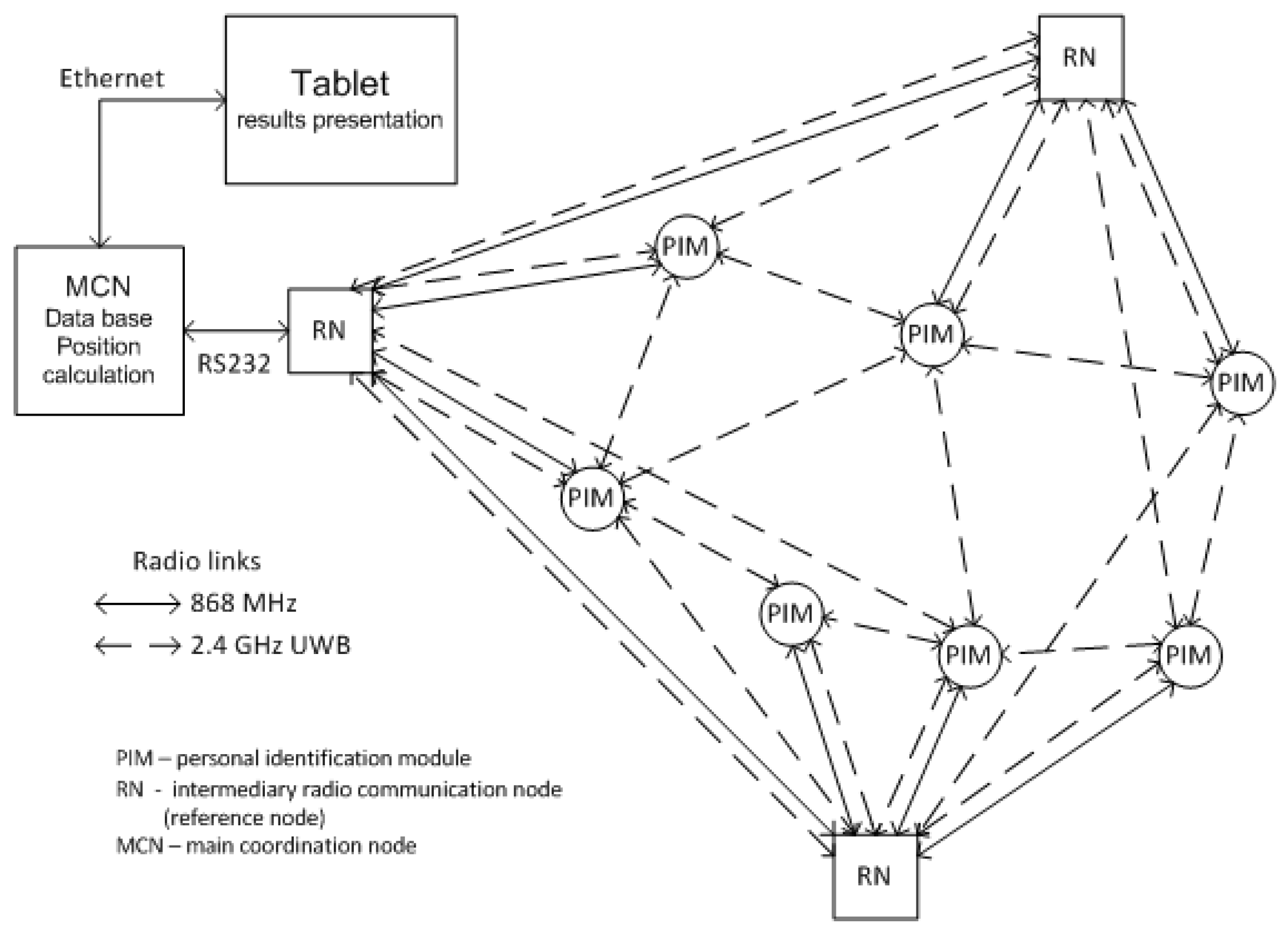
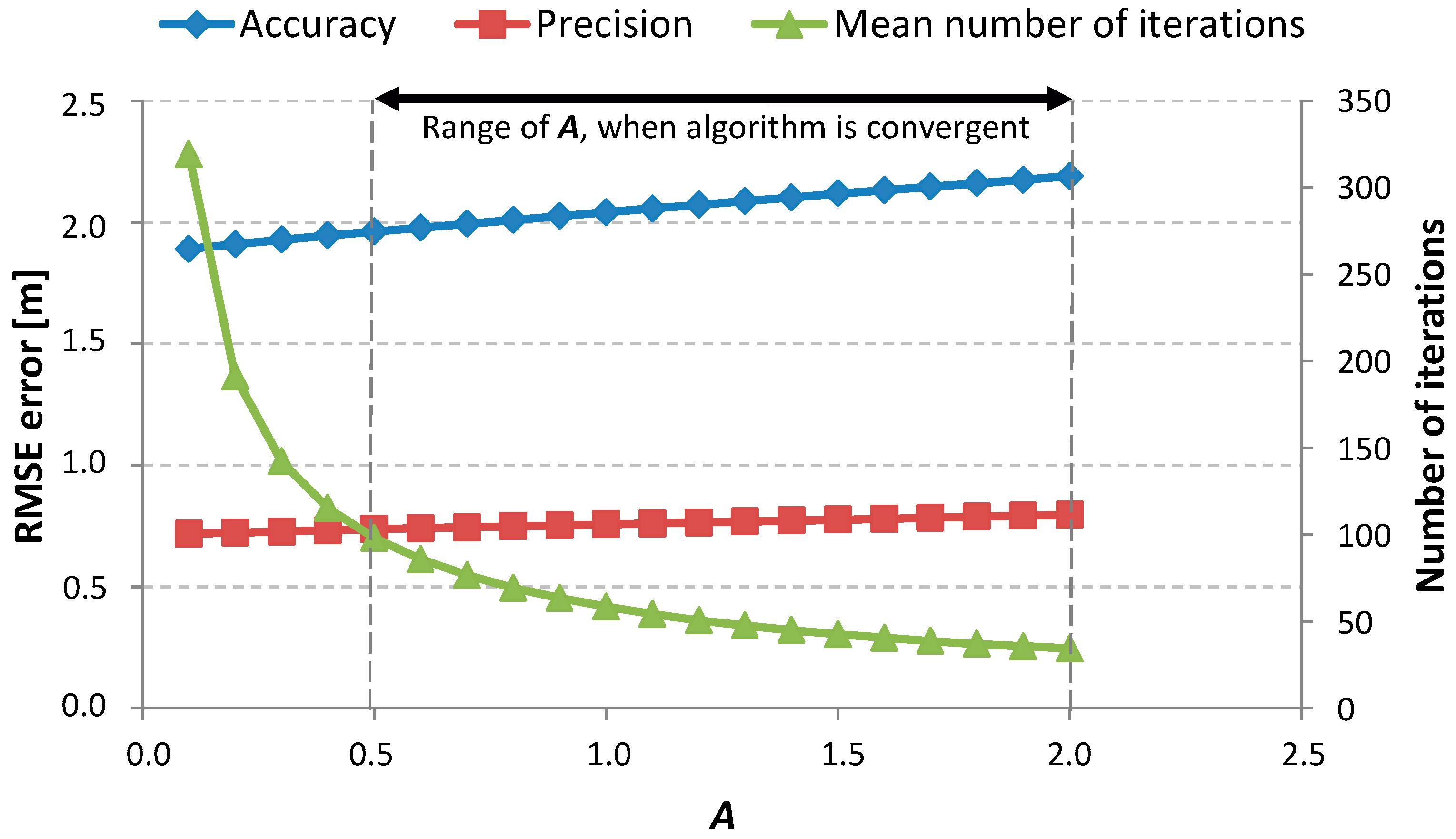
Figure 4 and Figure 5 are present the results for the calibration steps realized for a single-family, one-floor, inhabited house. In this scenario of measurements, all devices (PIMs and RNs) were deployed on the ground floor inside the building in different rooms. In the first step of calibration, $B$ was always set to 10. For this fixed $B$, the accuracy and precision of the positioning for a range of values of parameter $A$ were checked. The results of this step are presented in Figure 4. On the basis of these results, a value of $A$ was chosen. 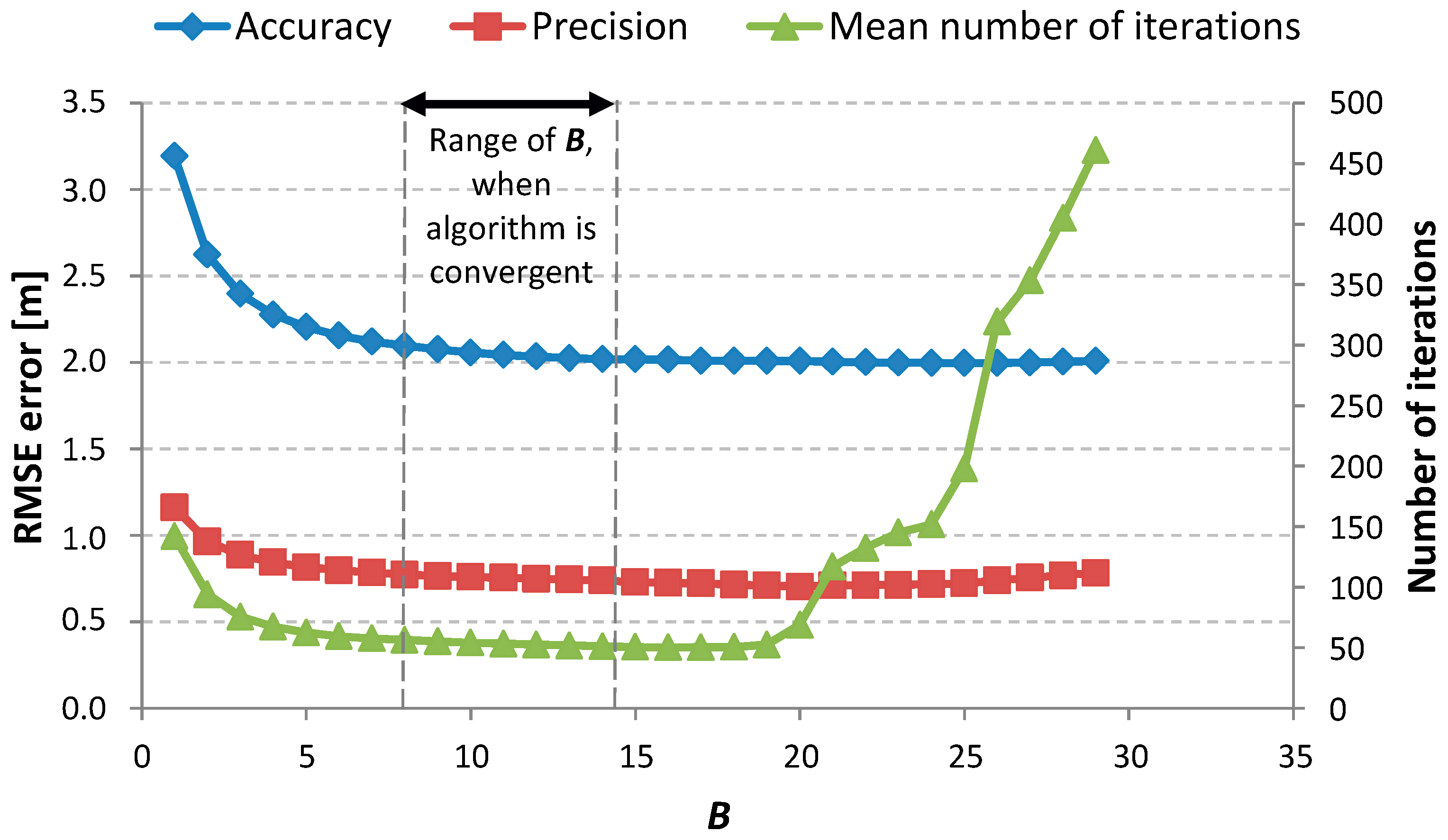For the chosen $A$, the value of $B$ was determined in a similar way. The results for the second step of calibration are presented in Figure 5.

For each measurement scenario, increasing the value of $A$ led to increasing values of accuracy and precision and simultaneously decreased the needed number of iterations. It is better when all of the considered values are the lowest. Low values of accuracy and precision mean good positioning properties and a low number of required iterations means that the algorithm returns the solution faster. To achieve good positioning performance, it would be best to choose the smallest value of parameter $A$. However, it must be noticed that if $A$ was smaller than a particular value (for this scenario, about 0.5, but in general it was different for each scenario) the algorithm became unstable. So, the chosen value must be greater than that particular one. As the precision and accuracy were growing alongside the value of parameter $A$, the decision was made to stop the first step of the calibration process for $A$ equal to 2.0. For this value, the mean number of iterations was sufficiently low and the results gained enabled us to choose a value of $A$. The chosen value $A$ is the lowest value (also the lowest are precision and accuracy values) for which the mean number of iterations is lower than 50. Additionally, for the $B$ parameter, it was observed that there was always a range of $B$ values for which the algorithm was stable and convergent. Moreover, there was always some threshold observed, such that until it was reached, the values of accuracy, precision, and mean number of iterations decreased. When the value of $B$ was greater than that threshold and increasing, the values of the considered parameters were also increasing. The mean value of iterations was calculated only for cases when the algorithm proved to be convergent. That is why, for values of $B$ in the ranges 1–7 and 15–20 in Figure 5, the mean value of iterations is relatively small despite the algorithm not being convergent. For the presented scenario, $A$ = 1.1 and $B$ = 14 were chosen. 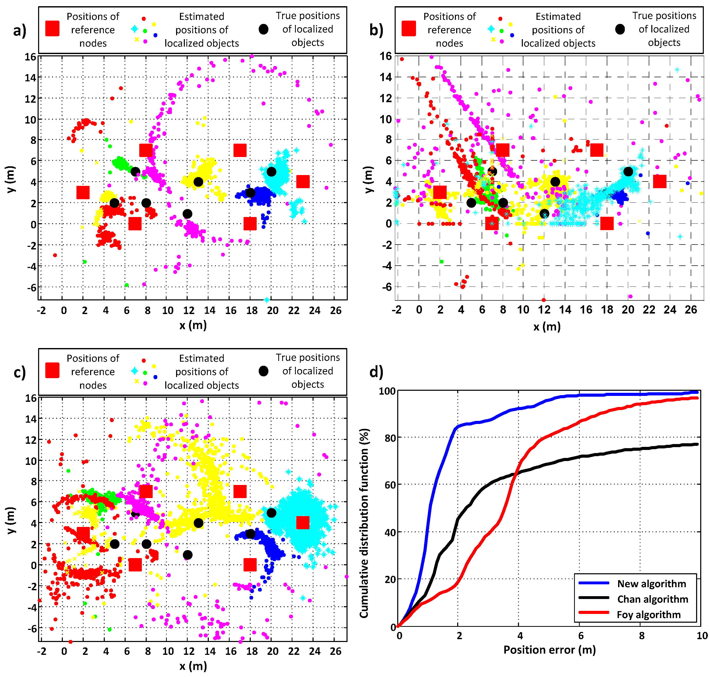For such parameters of $A$ and $B$, the estimated positions were calculated. 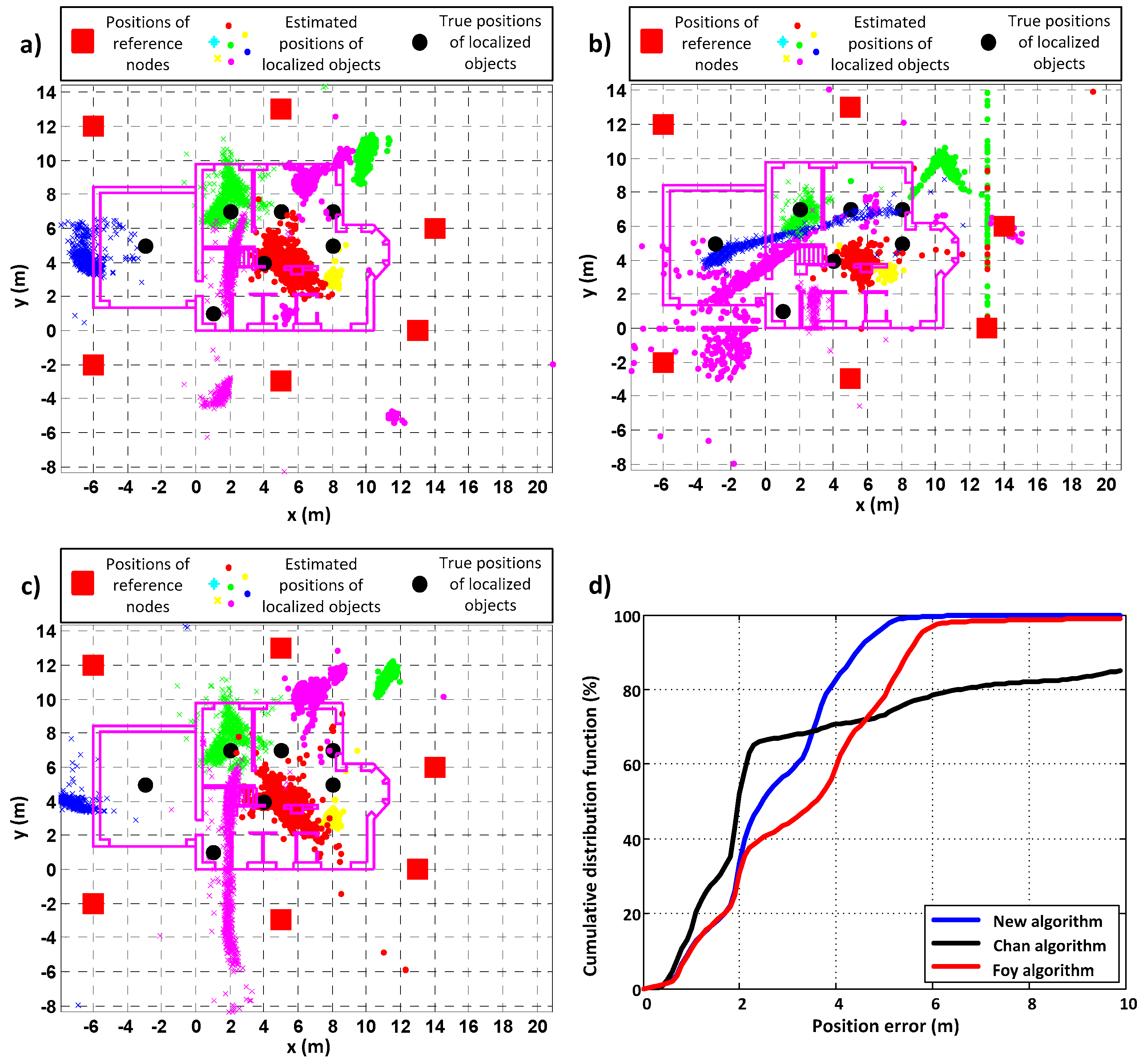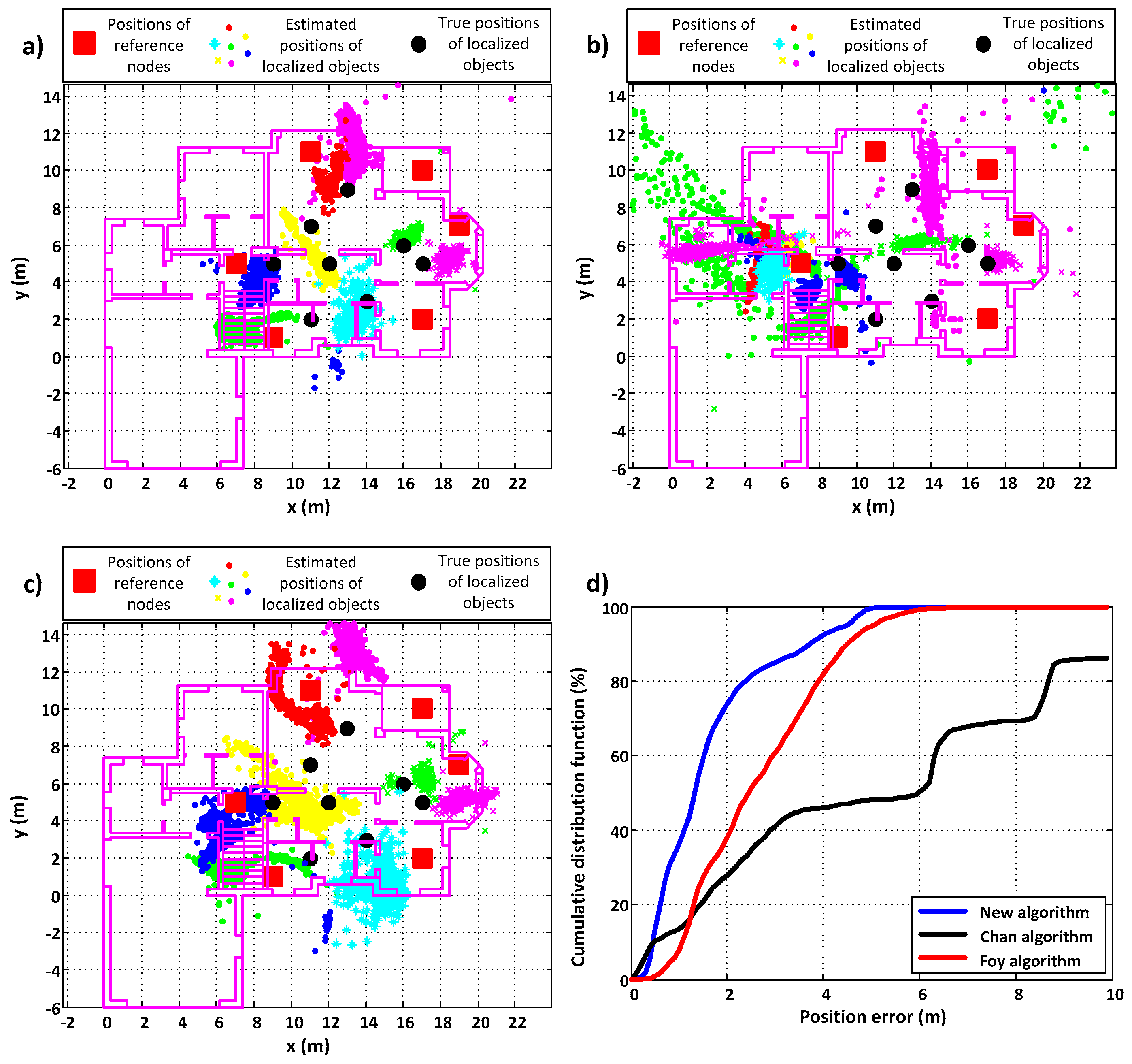The determined positions are presented in Figure 6a (color symbols). The outline of the building is also presented (violet lines). The black dots are places were PIM devices were deployed. The positions of RNs are marked by red squares. To conduct a comparative analysis with the performance of the Chan and Foy algorithms, the same calculations were made using those known algorithms. The results are presented in Figure 6b,c, respectively. In Figure 6d shows the cumulative distribution functions of the position errors for each algorithm.

Table 1. Results of comparative analysis when all devices where deployed inside an inhabited single-family house.

Analyzed Parameters	New Algorithm	Chan Algorithm	Foy Algorithm
RMSE accuracy (m)	2.04	8.92	2.97
RMSE precision (m)	0.78	6.35	1.18
Loss probability	0	5.9 × 10−4	0

presents the accuracy and precision errors for each algorithm. In the last row is given a loss probability parameter, which tells how probable it is that the given algorithm will not return a valuable result for the particular measurement data. Those results that are real numbers and lie within the area of interest are treated as valuable results.

From the given results, it may be seen that the proposed new algorithm gives the best results, i.e., the lowest values of accuracy and precision errors. What is more, it always returns a position, unlike the Chan algorithm for which the loss probability is greater than zero. As well, the cumulative distribution functions prove that the performance of the proposed algorithm is the best when compared to the Chan and Foy algorithms.

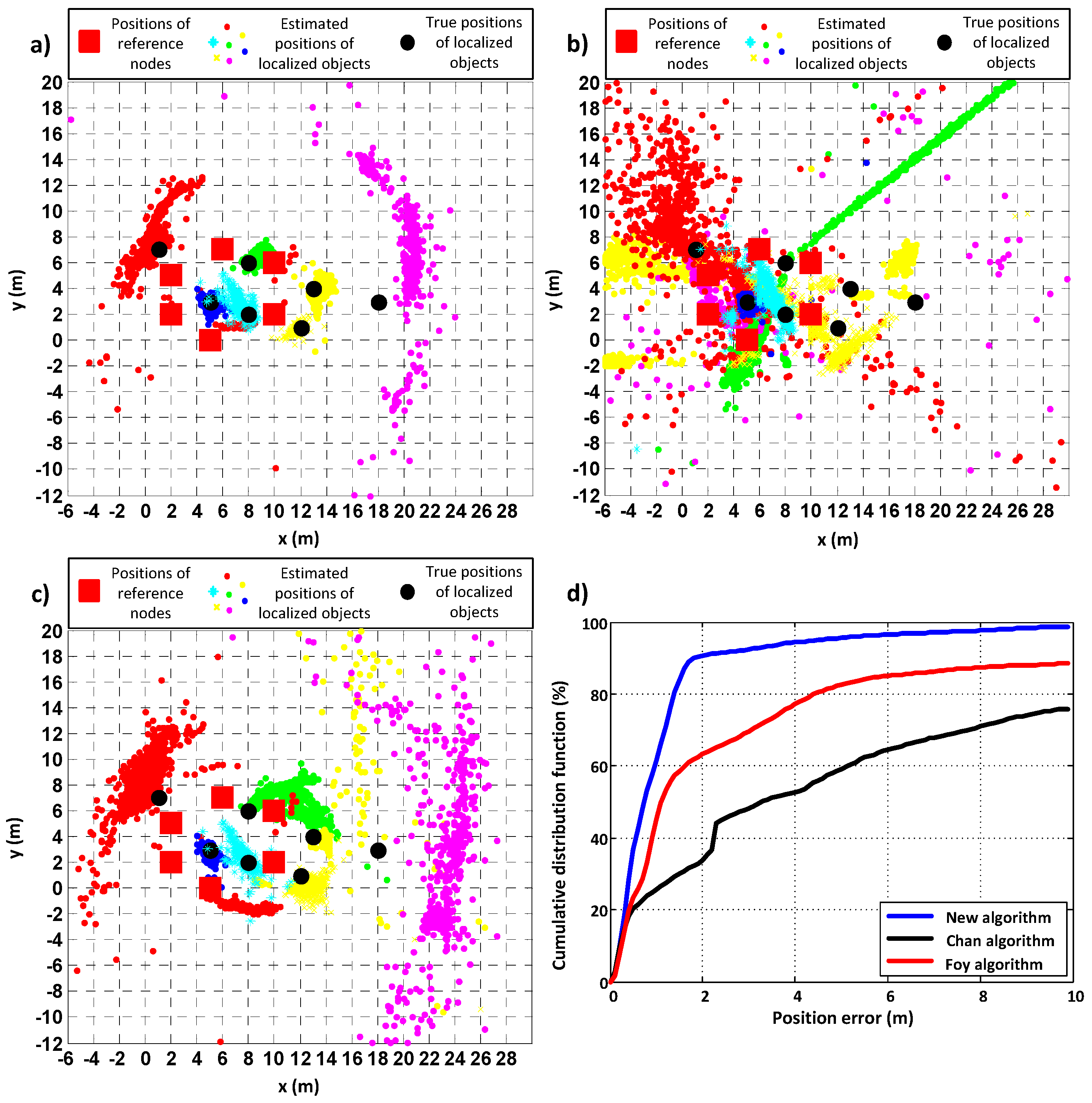
The above measurements were made in an inhabited single-family house when all devices were placed on one floor but in different rooms. Measurements were also made in a corridor with a few different arrangements of devices and in an un-inhabited single-family house (it was under construction). The plots for the results achieved by each algorithm when all devices where located in one corridor are presented in Figure 7. The six reference nodes in this case were placed along the walls and PIMs were inside the area confined by RNs to ensure good geometry. The good geometry is when reference nodes are evenly deployed around the area where localized objects are. When localized objects are outside this area, the geometry for them is poor. The further localized objects are from the area confined by reference nodes the poorer the geometry. The better the geometry, the greater the accuracy of positioning. The position errors for all compared algorithms for this series of measurements are presented in

Table 2. Results of comparative analysis when all devices were deployed within one corridor, with assurance of good geometry.

Analyzed Parameters	New Algorithm	Chan Algorithm	Foy Algorithm
RMSE accuracy (m)	2.42	12.36	5.50
RMSE precision (m)	1.83	11.09	4.49
Loss probability	0	0.0030	0.0026

. The $A$ and $B$ parameters in the proposed algorithm were set to 0.8 and 11, respectively.

Also in this scenario, the performance of the new algorithm is the best. Comparing the plots in Figure 7a–c, it can be noticed that the concentration of estimated positions is the greatest for the proposed algorithm. In addition, the values of accuracy and precision errors are the lowest for the proposed algorithm, which is also proven by the plot in Figure 7d. Moreover, the new algorithm gave a result for all sets of distance measurements, contrary to the Chan and Foy algorithms.

The performance of the algorithms was also checked in a scenario when all devices were placed in the same corridor but with poor geometry—when some PIMs were placed outside the area confined by the reference nodes. The results for this case are shown in Figure 8 and in

Table 3. Results of comparative analysis when all devices were deployed within one corridor with poor geometry.

Analyzed Parameters	New Algorithm	Chan Algorithm	Foy Algorithm
RMSE accuracy (m)	2.85	12.81	10.38
RMSE precision (m)	2.73	11.57	8.44
Loss probability	0	0.0022	0.0071

. For these measurements, in the proposed algorithm, parameter $A$ was equal to 0.8 and $B$ to 10.

In this scenario, as well, the proposed algorithm gives the best results—the values of errors are the lowest (almost 5 times better than the Foy algorithm and almost 6 times better than the Chan algorithm) and positions were calculated for all sets of distance measurements, while the loss probabilities for the Chan and Foy algorithms were greater than zero. In Figure 8a–c, it can be seen that the concentration of estimated positions around the true positions of PIMs is the greatest for the new algorithm. This is confirmed by the cumulative distribution function plot (Figure 8d).

Measurements were also conducted when PIM modules were located on the first floor (3.04 m above the ground) of the un-inhabited single-family house while the RNs were deployed outside the house. Figure 9 and

Table 4. Results of comparative analysis when PIMs were placed on the first floor of un-inhabited single-family house and RNs were deployed outside it.

Analyzed Parameters	New Algorithm	Chan Algorithm	Foy Algorithm
RMSE accuracy (m)	3.04	9.70	4.05
RMSE precision (m)	1.80	6.25	2.41
Loss probability	0	0.00184	0

show the results for this scenario. For these measurements, the parameters $A$ and $B$ for the proposed algorithm were set to 1.4 and 20, respectively.

As in the previous cases, the proposed algorithm outperformed the other two known algorithms. It gave the lowest values of accuracy and precision errors. The accuracy was better for the new algorithm by 25% when compared to the Foy algorithm and by almost 70%, when compared to the Chan algorithm. The proposed algorithm also returned positions for the entire set of distance measurements.

7. Conclusions

A new positioning algorithm was proposed herein. It was developed specifically for radio distance measurement methods realized in an indoor environment. The algorithm can be adjusted to the conditions of the propagation environment. The adjustment is made by changing the values of the coefficients of the ray slopes in the non-linear error function, which is the most important feature of the proposed algorithm.

What is more, the new algorithm, due to the utilization of simple mathematical calculations, always returns the calculated position, contrary to the popular Chan and Foy positioning algorithms, which utilize matrix inversion.

The performance of the proposed algorithm was compared to that of the Chan and Foy algorithms. The comparative analysis was conducted by using real distance measurements made in different environments, as follows: A corridor (two different scenarios) and two different single-family houses. For all cases, the proposed algorithm gave the best results, i.e., the smallest values of accuracy and precision errors. The improvement was greater than 25% when compared to the Foy algorithm and 65% when compared to the Chan algorithm. There were 20 other measurements also conducted in four different buildings and for all the cases the proposed algorithm turned out to be more accurate over dozens of percent compared to the Foy algorithm and tens of percent compared to the Chan algorithm.