Abstract
The term smart grid (SG) has been used by many government bodies and researchers to refer to the new trend in the power industry of modernizing and automating the existing power system. SGs must utilize assets optimally by making use of the information, like equipment capacity, voltage drop, radial network structure, minimizing investment and operating costs, minimizing energy loss and reliability indices, and so on. One way to achieve this is to re-route or reconfigure distribution systems (DSs). Distribution systems are reconfigured to choose a switching combination of branches of the system that optimize certain performance parameters of the power supply, while satisfying some specified constraints. In this paper, a blended biased and unbiased weightage (BBUW) multiple attribute decision-making (MADM) method is proposed for finding the compromised best configuration and compared it with other decision-making methods, such as the weighted sum method (WSM), weighted product method (WPM), and the Technique for Order Preference by Similarity to Ideal Solution (TOPSIS) method. The BBUW method is implemented for two distribution systems, and the result obtained shows a good co-relationship between BBUW and other decision-making methods. Further weights obtained from the BBUW method are used for the WSM, WPM and TOPSIS methods for decision making. Examples of the distribution system are worked out in this paper to demonstrate the validity and effectiveness of the method.
1. Introduction
The electric power system is a vital part of modern developed societies. Electric power systems are mainly divided into three parts: generation, transmission and distribution. A distribution system (DS) is the tail end of the utility, and delivers electrical power to consumers. Due to the competitive environment and deregulation policies in the power sector, distribution companies are under continuous stress to curtail operating costs by minimizing active power losses and improving reliability and other parameters to affect the performance. This has forced power system managers to make use of innovative practices to contribute to the evolution of the power system into the smart grid. Smart grids (SGs) are modern, intelligent systems that consist of sensors and monitoring mechanism, such as information and communication technologies (ICT), to give better performance and to provide good economic service to consumers. Smart grids should be more reliable, more secure, more economical, more efficient, more environment friendly and much safer than conventional power systems.
A distribution system is mainly reconfigured for improving the reliability of the system, to balance the load on the feeders, to get relief from overloads, to minimize the power loss, to improve the voltage profile, and so on. In distribution systems, air break-type switches or sometimes circuit breakers are used for shifting the load from one feeder to another during fault conditions to maintain the reliability of the supply. Some of the switches are normally open (NO), and some are normally closed (NC). NO switches are known as sectionalizing switches, and NC switches are tie switches.By changing the position (ON/OFF) of sectionalizing switches and tie switches, the configuration or path can be changed or modified. Reconfiguration is altering of the topology of a network by changing the open/closed condition of NO/NC switches. Reconfiguration is done to improve the performance of the distributions system [1,2,3,4,5,6,7,8,9,10] through parameters like losses, reliability indices, voltage profile, and so on.
In ref. [1], feeder reconfiguration is done for loss reduction and load balancing by using the branch exchange method. In ref. [2], switches were opened one by one starting in a closed mesh, and the optimal power flow method is used. An algorithm is developed based on optimal flow pattern, for a single loop formed by closing a normally open switch, and the process is repeated until minimum loss configuration is reached [3]. A genetic algorithm is used for the first time for minimum loss reconfiguration methodology in a distribution system [4].
The heuristic method starts with all switches open, and at every step the switch results in the least increase of the closed objective function [5]. A heuristic-based fuzzy multi-objective algorithm is proposed [6] to solve the network reconfiguration problem in a radial distribution system. A technique at the low-voltage and medium-voltage (MV) levels of a distribution network, employed simultaneously with reconfiguration at both levels, is proposed in [7], and the neural network is adapted for the network reconfiguration problem. A harmony search algorithm (HSA) is used to solve the network reconfiguration problem to get the optimal switching combination in the network, which results in minimum loss [8]. In ref. [9], a reconfiguration methodology considering reliability and power loss is proposed. The optimal status of the switches in order to maximize reliability and minimize the real power loss is found using a binary particle swarm optimization (BPSO) algorithm. In ref. [10], a method is proposed to improve the reliability of the distribution system using the reconfiguration strategy and a clonal selection algorithm for optimization.
There are several important SG aspects, such as field sensors, ICT technologies and data collection equipment. Such elements are very relevant for the real feasibility of the considered application in a distribution system. In fact, they are crucial for the correct operation of network reconfiguration, measurement uncertainties, meter placement, communication and data collection issues, which can negatively affect decision-making performance. State estimation, power flow monitoring and control play a vital role in distribution systems, and in the worst case they can lead to wrong results.
In ref. [11], a method for meter placement for improving the voltage quality and its angle in a distribution network is proposed. This method uses a bivariate probability index to control relative errors at each bus voltage and its angle. In ref. [12], the problem of meter placement for distribution system state estimations is discussed. This method is based on exact calculations of probabilities, as compared to the method proposed in ref. [11] in which estimated probabilities are used. A power-flow analysis in medium-voltage (MV) networks, based on load power measurements at a low-voltage level, is modified by considering the temporary unavailability of power measurement [13]. Also, an artificial neural network (ANN)-based load-power estimation method is used. Measurement device placement in low-voltage (LV) distribution systems for load-flow analysis in medium-voltage distribution systems is proposed in ref. [14]. This method finds the number and location of measurement devices considering the uncertainty of power flow estimation. The two-stage methodology for finding the optimal location for placing a monitoring device instrument with minimum investment cost using differential evolution (DE) and particle swarm optimization (PSO) is proposed in ref. [15]. A second-stage real-time measurement to estimate the bus voltage is proposed, which is required for decision making.
For effective monitoring and controlling of distribution system meters are required to ensure they are placed optimally and economically. A brief review of meter placement and artificial intelligence algorithms is proposed in ref. [16] by considering various constraints. Distribution system operators (DSOs) face many problems due to uncertainty while making decisions. In ref. [17], an optimal power flow based on information gap decision theory is proposed. An internet protocol (IP)-based communication with power line communication (PLC) is proposed to get to the last point (i.e., smart meters, etc.) [18]. An internet of things (IoT)-based distribution system cyber security is of prime importance. In ref. [19], a decentralized energy management framework is proposed for decision making in distribution systems.
In decision making [20,21,22,23], numbers of alternatives or options are considered along with some attributes or criteria that are compared, processed and ranked. A decision table or matrix consists of number of alternatives and attributes. It also considers weightage or relative importance of attributes, as well as dealing with performance amongst alternatives, as described in refs. [20,21,22,23]. A decision maker’s (DM’s) main job is to get a compromised best from the given alternatives.
A traditional optimization approach in electrical distribution systems is to find the solution with the minimum cost, though in ref. [24] the authors propose a methodology that evaluates a number of criteria by using the multiple-criteria decision-making (MCDM) method to trade-off between alternative solutions. Reconfiguration of distribution systems with Pareto front analysis is done by considering network losses and energy not supplied as multi-objectives [25]. MCDM methods are helpful in finding the solutions to problems having multiple or conflicting objectives. A review of the literature was done to analyze the various methods, and it was found that the analytical hierarchy process (AHP), preference ranking organization method for enrichment evaluations (PROMETHEE) and elimination and choice translating reality (ELECTRE) were the most popular methods [26].
Reconfiguration of distribution is done for various purposes. After the reconfiguration of distribution system, available alternatives are different switching combinations for decision-making. The attributes that may be considered for decision making are energy losses, security of system, voltage magnitude, capital cost, supply availability or non-availability, constraints related to capacity, length of the circuit and reliability indices such as system average interruption frequency index (SAIFI), system average interruption duration index (SAIDI), consumer average interruption frequency index (CAIFI), customer average interruption duration index (CAIDI) and average energy not supplied (AENS) [27,28].The application of multiple attribute decision-making (MADM) methods for decision making in distribution systems is described by PROMETHEE [29], which is improved upon as AHP–PROMETHEE [30]. An evaluation of Technique for Order Preference by Similarity to Ideal Solution (TOPSIS) and PROMETHEE [31], and a comparison of the simple additive method (SAW) or weighted sum method (WSM), weighted product method (WPM) and TOPSIS and PROMEHEE methods is done in [32].
Generally, there are two methods for determining attribute weights—biased (or subjective) and unbiased (or objective). The important aspect in decision making is that the weights are determined by experts. In an unbiased or objective method, there are also some biased or subjective factors to be considered. The unbiased weightage method has the advantage of having information about attributes to decide weights, and does not depend on the biased judgment of decision makers. The weights are assigned by applying a mathematical method to attributes.
In a biased weightage method, weights are assigned to attributes as per the experience of the decision maker, who should have experience and the field. A decision maker’s experience can be very useful in deciding the biased or subjective weight method, but it should not be at the cost of losing its flexibility and mutability, as doing so can lead to randomness. In an unbiased or objective weight method, subjective will is not considered, and therefore it can be inconsistent with the actual importance of given attributes and it may be difficult to explain the results obtained.
Researchers must take advantage of and overcome the limitations of the combined biased and unbiased weights, but methods must be chosen to determine unbiased and biased weightages, or which methods can be combined, to overcome the limitations of either the biased or unbiased approach.
In this paper, a blended biased and unbiased (BBUW) method is proposed for obtaining the compromised optimal combination of switches by considering some of the attributes from available alternatives for practical distribution systems, and the results are compared with other MADM methods such as WSM, WPM, AHP and TOPSIS [27,28,29,30,31,32].
2. Decision-Making Methods
Decision making plays an important role in utilizing all the resources optimally and efficiently in any organization. A manager’s target is to achieve the maximum possible productivity with available resources for achieving predefined goals. In a real-life situation, decisions have to be made under complicated conditions with various criteria/attributes that may contrast with each other, resulting in a more-challenging task. The development of logical and systematic methods is required for assisting decision makers in consideration of various attributes and their interrelations. The job of a decision maker is to find and get the best mixture of suitable attributes.
It is essential to cautiously examine attributes before choosing an alternative for the desired purpose. The attributes are classified in two categories:
- beneficial attributes (attributes where the higher values preferred are beneficial attributes, such as efficiency, profit and so on);
- non-beneficial attributes (attributes where lower values are favored, such as losses, cost of purchase and so on).
2.1. Multiple Criterion Decision-Making (MCDM) Methods
Multiple criterion decision-making (MCDM) methods can be used for solving multiple criteria problems, and are categorized as
- multiple objective decision-making (MODM) methods;
- multiple attribute decision-making (MADM) methods.
MODM methods are applicable when there are several objectives, and decision maker has to decide the best without violating limits.
MADM methods are used to solve decision-making problems associated with a number of predetermined alternatives. In cases of complicated problems where multiple factors are considered, multi-attribute decision-making (MADM) methods are preferred by researchers or decision makers.
In MADM, the number of alternatives and shortlisted attributes are processed with some logical, analytical methods, and ranked, and the final decision is made by considering the practical knowledge of the decision maker and their experience.
2.2. Multiple-Attribute Decision Making (MADM)
Every decision matrix or decision table in MADM consists of shortlisted alternatives, attributes, weightage or significance of each attribute and performance measure for the alternatives. The decision matrix or table can be prepared as given in Table 1. The decision matrix or table comprises alternatives Ai (for i = 1 to N), attributes Bj (for j = 1 to M), weightages considered for attributes wj (for j = 1 to M) and performance measures for alternatives mij (for i = 1 to N; j = 1 to M) [20].

Table 1.
Decision table or matrix in MADM methods.
The decision maker needs to choose the best alternative from the available or shortlisted alternatives from the decision matrix. Many times units of the considered attributes are altogether different, hence it is required to normalize them so that they are on same platform.
Some of the popular multi-criteria decision-making methods used for decision making are
- (i)
- analytic hierarchy process (AHP);
- (ii)
- weighted product method (WPM);
- (iii)
- weighted sum method (WSM);
- (iv)
- elimination and choice translating reality (ELECTRE);
- (v)
- Technique for Order Preference by Similarity to Ideal Solution (TOPSIS);
- (vi)
- Višekriterijumsko kompromisno rangiranje (VIKOR);
- (vii)
- preference ranking organization method for enrichment evaluations (PROMETHEE).
2.3. Blended Biased and Unbiased Weightage (BBUW) MADM Method
A blended biased and unbiased weightage (BBUW) multi-attribute decision-making (MADM) method is proposed in this section. Unbiased weightage of significance with respect to attributes and the biased priority of preference of the DM are considered collectively to find the aggregated or integrated weightages of the pre-determined attributes. This BBUW method assists the DM to reach a decision by using (a) the biased weightage of significance for the attributes, (b) the unbiased priority of preference or (c) taking into account both (a) and (b).
Table 1 shows the general arrangement of alternatives and attributes for decision-making problems.
The steps to be followed in decision making for a given distribution system problem using the blended biased and unbiased weights (BBUW) method [23] are as follows:
- Step 1:
- Identify and curtail the alternatives by considering the criteria.
- Step 2:
- Arrange a decision matrix or table after short listing the alternatives and values related to the attributes (mij).
- Step 3:
- The values of the attributes (mij) are generally in different units (e.g., losses in Mwh, cost in Rupees, etc.). Hence, it is necessary to list all parameters of the decision table or matrix for different alternatives on a common platform. Obtain the normalized decision matrix mij* by using Equation (1).where, mij* is the normalized value of mij and N, and ∑ mij is the sum of the of jth attribute values for alternatives (from i =1 to N).
- Step 4:
- The weightages of relative significance of the attributes can be determined by the decision maker for the given example based on three parameters: (a) biased weights of alternatives, (b) unbiased weights of the attributes or (c) integration of both (a) and (b).
- (a)
- Unbiased weightage of significance of the attributes: In this paper, the statistical variance considered for determining the unbiased or objective weightage of significance of the attributes is calculated using Equation (2).where, Vj is the statistical variance for the jth attribute, and (mij*) mean is the average value of mij*. Range considers the extreme points, but the variance considers all points and then finds their distribution. Hence, the variance provides important information regarding the data distribution.The unbiased weightage of the jth attribute (wjU) can be calculated by separating the variance of the jth attribute with the total variance value with M attributes. Thus, wjU can be found using Equation (3).
- (b)
- Biased weightage of significance of the attributes: The weightage of relative significance of the attributes can be determined on the basis of a DM’s choice for the attributes for a given application, or by using any other method.
- (c)
- Blended weightage of significance of the attributes: The DM can integrate the unbiased and biased weightage of the attributes using Equation (4).where, is the integrated or aggregated weight of the jth attribute, WB is weightage assigned to the biased weights and WU is the weightage assigned to the unbiased weights. By integrating WB and WU, the decision maker decides the importance of unbiased and biased weights.
- Step 5:
- Every considered attribute is allocated a weightage that can be unbiased, biased, aggregated or integrated. Data corresponding to each attribute are processed with respect to each alternative. The performance index (Pi) is calculated using the weightage sum method by considering the general performance of the shortlisted alternative.The performance index for every alternative shows the merit of the alternative in comparison with all the other alternatives. Performance index (Pi) is calculated using Equations (5)–(7).where, mij** = [mij*b/(mij*b)max] for beneficiary attributes, and [(mij*nb)min/mij*nb] for non-beneficiary attributes; mij*b and mij*nb signify the normalized values of the beneficiary and non-beneficiary attributes, respectively; (mij*b)max is the greatest value of the jth beneficiary attribute; and (mij*nb)min indicates the smallest value of the jth non-beneficiary attribute.Equation (5) can be used to calculate the unbiased or objective weightage of the attributes; Equation (6) is used for the biased or subjective weightage of the attributes; and Equation (7) is used for the aggregated or integrated weightage of the attributes.
- Step 6:
- Arrange the solutions or alternatives in a descending order as per values of the preference index. The highest preference index value of an alternative is preferred as rank1 for the given decision-making problem.
- Step 7:
- Finally, considering the practical limitations and other constraints, the DM can arrive at the conclusion, but preference is given to the alternative with the maximum value of the preference index.
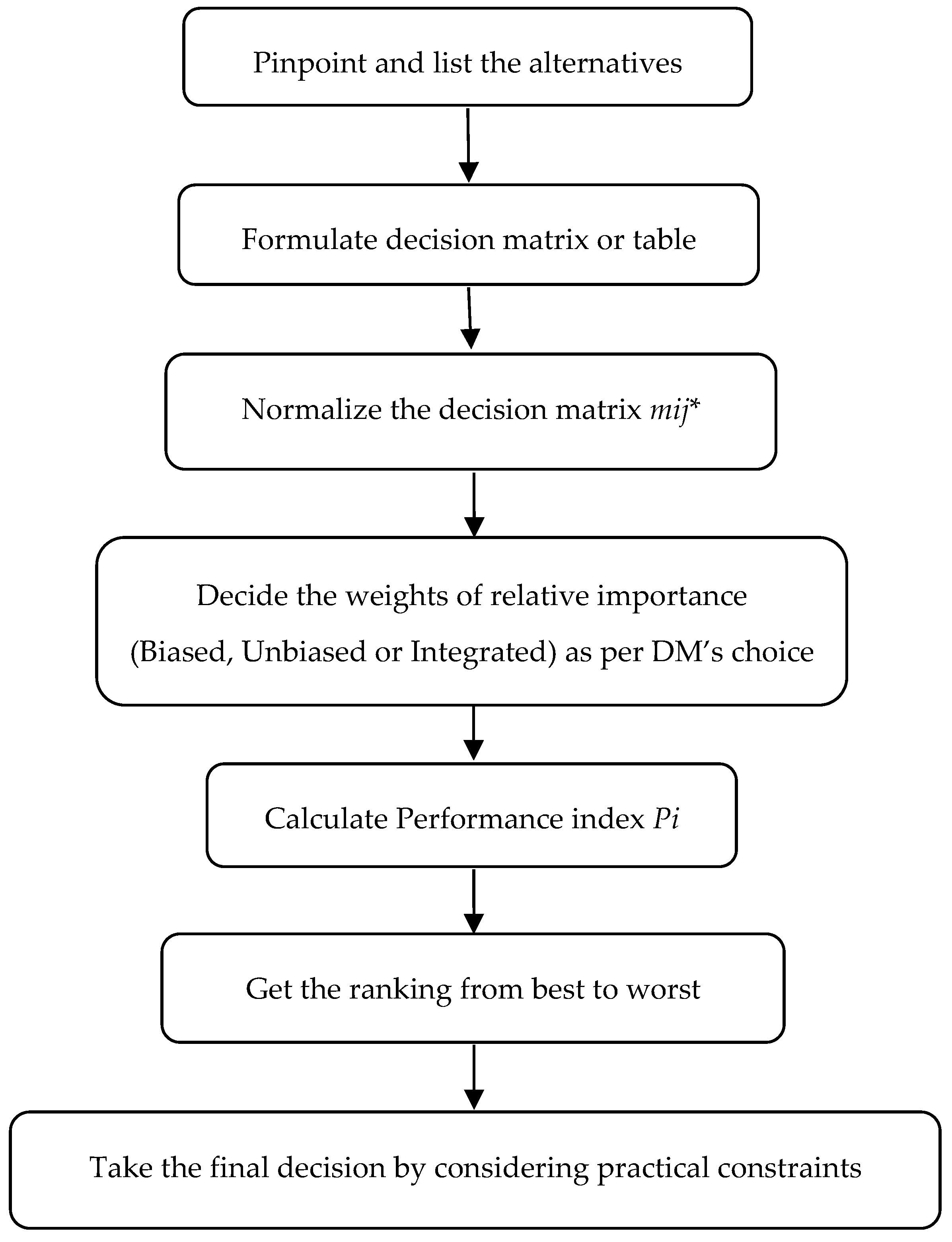
Figure 1 depicts the flow chart for the proposed BBUW MADM method.
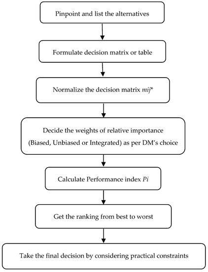
Figure 1.
Flow chart for the blended biased and unbiased weightage (BBUW) MADM method.
3. Implementation and Results
3.1. Distribution System Case Study 1
The case study of a 33-bus system, rated at 12.66 kV, is considered from [27]. The total power demand was 3715 kW and 2000 kVAR. The total number of customers on the given distribution system was 18,200. Further details for the considered distribution system can be obtained from [27]. There are many feasible switching combinations or configurations in the study; out of these, only non-dominated alternatives are shortlisted, as provided in the Table 2. The biased or subjective weightage of the attributes given for this case were 0.3 for the active power losses, 0.35 for SAIFI and 0.35 for AENS.
Table 2.
Data for distribution system case 1 [27,31].
There are 14 shortlisted alternatives or solutions available for the decision maker, and three attributes considered: active power losses, SAIFI and AENS. All of these attributes are non-beneficial (i.e., should be as minimal as possible to get the utmost benefit for the distribution system).
Application of Blended Biased and Unbiased Weightage (BBUW) Method for Decision Making in Smart Distribution System Case Study 1:
The following procedure is followed for decision making by using the blended biased and unbiased (BBUW) MADM method:
- Step 1:
- The selection attributes identified for selecting the optimal switching combination are energy losses, SAIFI and AENS.
- Step 2:
- The decision table or matrix is prepared and entered into Table 2.
- Step 3:
- The data is normalized by using Equation (1), as the attributes have different units in Table 3.
Table 3. Normalized values.
- Step 4:
- The weightage of relative importance of the attributes can be worked out by the DM for any one of the following:
- (a)
- The unbiased weightages of the attributes are calculated with the help of Equations (2) and (3) as follows:0.4814, = 0.2543, = 0.2643.
- (b)
- The biased weightages are taken from ref. [27] to compare the results:= 0.3000, = 0.3500, = 0.3500
- (c)
- The blended or integrated weights (as per significance of the attributes) are calculated with the help of Equation (4) and displayed in Table 4 for the different combinations of weightages assigned to the unbiased and biased weightages of the considered attributes.
Table 4. Integrated or blended weights for different combinations.
- Step 5:
- The preference index numbers are calculated for various alternatives using Equations (5)–(7), and are listed in Table 5.
Table 5. Preference index for different weights.
- Step 6:
- Alternatives are ranked as per preference index Pi values, with the highest Pi as rank 1 and so on (see Table 6).
Table 6. Rankings of solutions for the BBUW method (blended biased and unbiased weightage, BBUW).
- Step 7:
- A decision may be finalized considering the practical limitations by the decision maker using their knowledge and experience as per the ranking marked.
The weights obtained from the BBUW method (see Table 4) are considered as weights for the other MADM methods WSM, WPM and TOPSIS. Table 7 and Table 8 show the results obtained by WSM and WPM for different weights respectively. Table 9 displays the results obtained by the TOPSIS method for different combinations of weights for case study 1.
Table 7.
Result of WSM for different weights (weighted sum method, WSM).
Table 8.
Result of WPM for different weights (weighted product method, WPM).
Table 9.
Result of TOPSIS method for different weights (Technique for Order Preference by Similarity to Ideal Solution, TOPSIS).
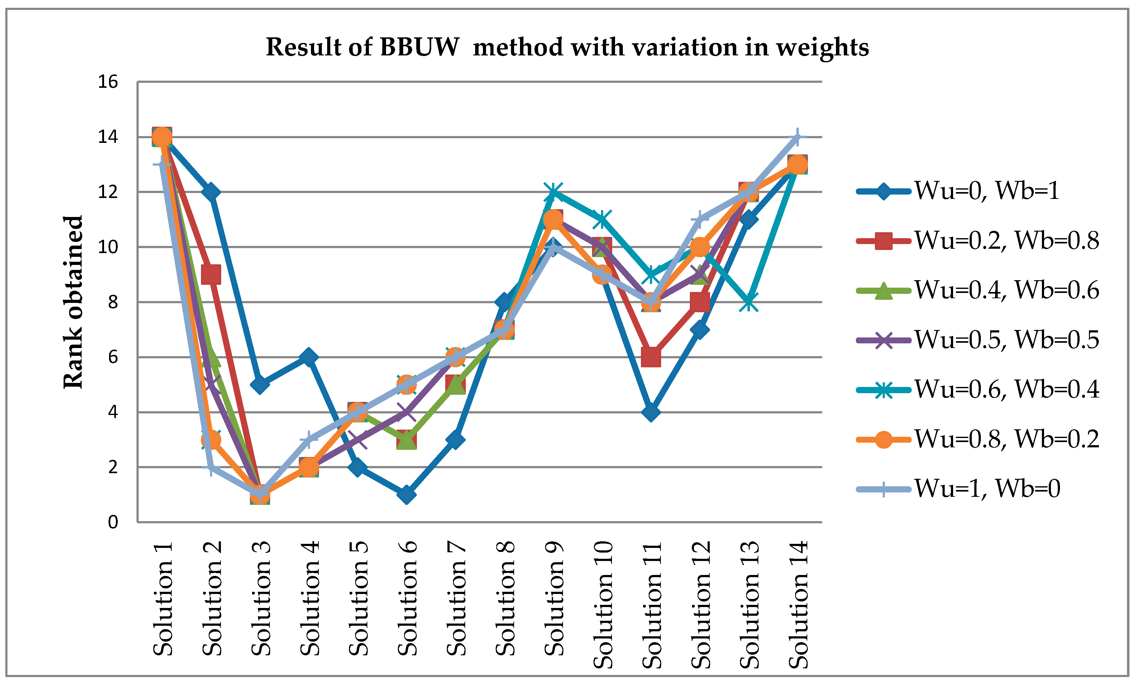
Results of the BBUW method for distribution system case study 1 are shown graphically in Figure 2.
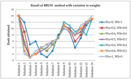
Figure 2.
Result of the BBUW method for distribution system case study 1.
3.2. Distribution System Case Study 2
Another case study considered is distribution system of a practical electricity utility from [28]. The proposed blended biased and unbiased weightage (BBUW) methodology is implemented on this case study. The considered distribution network consists of seven load points and 17 transformers along with underground cables and overhead distribution lines of the rated voltage 11 kV. In this example, five alternatives or solutions are available for the decision maker, and six attributes are considered: system security, capital cost, supply availability, annual energy losses, circuit length and capacity constraints. All of the attributes shortlisted in this example are non-beneficial (i.e., minimum values are preferred for the benefit of the system).
Application of the Blended Biased and Unbiased Weightage (BBUW) Method for Decision Making in Smart Distribution System Case Study 2
The following procedure is followed for decision making using the blended biased and unbiased weightage (BBUW) MADM method:
- Step 1:
- The selection attributes identified for selecting the optimal switching combination are system security, capital cost, supply availability, annual energy losses, circuit length and capacity constraints.
- Step 2:
- The decision matrix or table is prepared, as given in Table 10.
Table 10. Distribution system case 2 [28].
- Step 3:
- The data is normalized using Equation (1), as the attributes have different units in Table 11.
Table 11. Normalized data for Distribution System case 2.
- Step 4:
- The decision maker can decide the weightage of relative significance for the considered attributes with one of the following method:
- (a)
- The unbiased or objective weightages of the attributes can be calculated with the help of Equations (2) and (3) as follows:WUEL = 0.000007, WUSS = 0.001784, WUSA = 0.014261, WUCCONS = 0.795030, WUCL = 0.187471, WUCCOST = 0.001446.
- (b)
- The biased or subjective weightages for the given example are taken from reference [28]:WBEL = 0.05, WBSS = 0.15, WBSA = 0.15, WBCCONS = 0.25, WBCL = 0.15, WBCCOST = 0.25.
- (c)
- The blended, or aggregate or integrated weightage of significance of the attributes are calculated with the help of Equation (4) and shown in Table 12 for various weightages assigned to the unbiased and biased weights for the considered attributes.
Table 12. Blended or integrated weights for different combinations.
- Step 5:
- Calculate the preference index values for different solutions or alternatives with the help of Equations (5)–(7), listed in Table 13.
Table 13. Preference index for different weights.
- Step 6:
- Rank the alternatives as per the values of preference index Pi, with the highest Pi ranked as 1 and so on (as shown in Table 14).
Table 14. Ranking of solutions.
- Step 7:
- A decision may be finalized considering the practical limitations by the decision maker using their knowledge and experience as per the ranking marked.
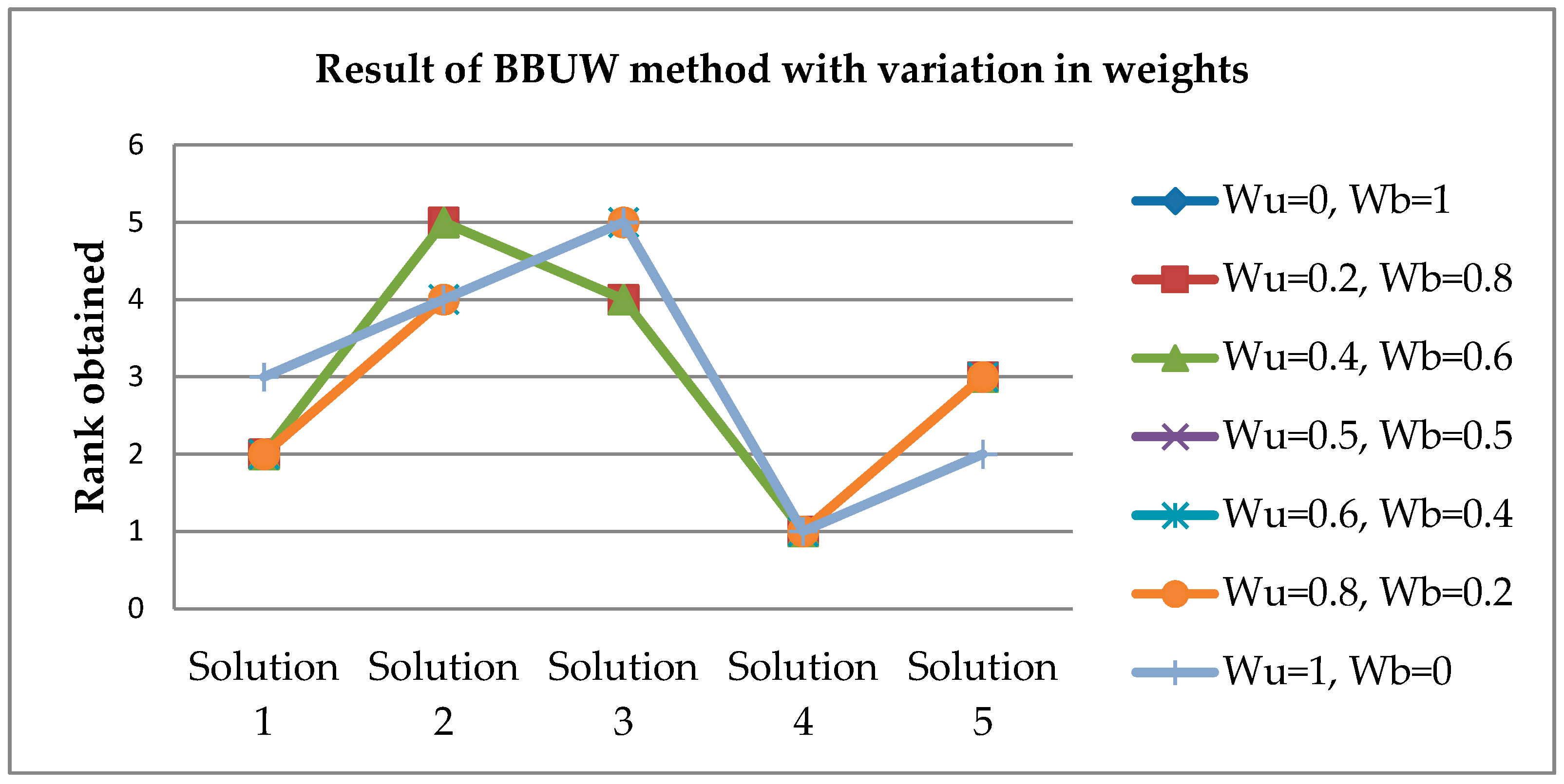
The weights obtained from the BBUW method (see Table 12) are considered as weights for the other MADM methods WSM, WPM and TOPSIS. Result of the BBUW method for distribution system case study 2 is shown graphically in Figure 3. Table 15 and Table 16 show the results obtained by WSM and WPM for different weights, and Table 17 displays the results obtained by the TOPSIS method for different combinations of weights for case study 2.
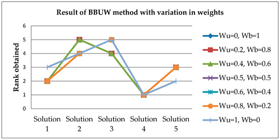
Figure 3.
Graphical representation of the results of the BBUW MADM method for distribution system case 2.
Table 15.
Result of WSM for different weights.
Table 16.
Result of WPM for different weights.
Table 17.
Result of TOPSIS method for different weights.
The two examples presented above demonstrate and validate the BBUW method as a prospective decision-making method for dealing with distribution system problems.
4. Results and Discussions
MADM methods use biased or subjective and unbiased or objective methods to determine weights. In some studies, researchers have combined biased and unbiased weights. In this paper, a blended biased and unbiased weightage (BBUW) MADM method was elaborated in detail considering statistical variance. In order to carry out a more complete analysis, the biased and unbiased weights were varied, and their effects on solution ranking were studied for the considered case studies. This was done to provide flexibility, as sometimes the priorities of distribution system operators may change due to changes in configuration or other alterations in infrastructure. In the literature available, weights were not varied for the considered case studies, thus the results of the present cannot be compared with them. Further, the weights obtained from the BBUW were taken as the inputs for the WSM, WPM and TOPSIS methods, and ranking was done accordingly for different combinations of biased and unbiased weights.
Other MADM methods, WPM, WSM and TOPSIS, were worked out to study and compare for two distribution network case studies to support in decision making. The attributes considered for the first case study reduced power losses in the system and minimized reliability parameters, such as SAIFI and AENS. The results of the BBUW and all other MADM methods were compared and arrived at the conclusion that alternative number 3 should receive rank 1 in WPM, WSM, TOPSIS and the proposed BBUW method. As anticipated, the rankings of the solutions were opposites, indicating that reliability and losses of these attributes were conflicting with each other. When the weights varied from 0 to 1, from unbiased to biased, rank 1 was obtained for solution 3, the first 7 positions were solutions 2–8 and the last ranking was different. The validation was done by comparing the results of the BBUW with the WSM, WPM and TOPSIS methods.
For the distribution network in cast study 2, the attributes considered were system security, capital cost, supply availability, annual energy losses, circuit length and capacity constraints. All the attributes were almost conflicting. The results of the BBUW and all other MADM methods were compared and arrived at the conclusion that alternative number 4 should receive rank 1 for the WPM, WSM, TOPSIS and proposed BBUW methods. Other rankings obtained by the BBUW method and other methods used in this paper were almost the same, hence the results are verified and validated.
The main advantage of this method is that it makes use of a DM’s experience, and deciding biased (or subjective) weights and unbiased (or objective) weights is accomplished using a mathematical model of statistical variance. The limitations of the work are that this method is applicable only to balanced distribution networks, and it does not consider the effects of distributed generation energy sources in the system. These issues are left for future studies to resolve. Sensitivity analysis can also be performed in the future.
5. Conclusions
The proposed blended biased and unbiased weightage (BBUW) method is very simple to understand, convenient to implement for any type of decision-making problem and comes under the umbrella of the weighted sum method. The described BBUW method assists the DM to arrive at a decision by considering (a) unbiased or objective weights, (b) biased or subjective weights or (c) blended or integrated unbiased and biased weights. The results obtained using the explained BBUW method show a good interrelation with other MADM methods. The overall approach of this paper is to provide the decision maker an effective solution among the different alternatives.
Author Contributions
The conceptualization, methodology, by S.G.K., K.V., data and analysis, writing and editing were conducted by S.G.K. and U.V.P., and Supervision by K.V. and U.V.P.
Funding
This research received no external funding.
Conflicts of Interest
The authors declare no conflict of interest.
References
- Baran, M.E.; Wu, F.F. Network reconfiguration in distribution systems for loss reduction and load balancing. IEEE Trans. Power Del. 1989, 4, 1401–1407. [Google Scholar] [CrossRef]
- Shirmohammadi, D.; Hong, H.W. Reconfiguration of electric distribution networks for resistive line losses reduction. IEEE Trans. Power Syst. 1989, 4, 1492–1498. [Google Scholar] [CrossRef]
- Goswami, S.K.; Basu, S.K. A new algorithm for the reconfiguration of distribution feeders for loss minimization. IEEE Trans. Power Del. 1992, 7, 1484–1491. [Google Scholar] [CrossRef]
- Nara, K.; Shiose, A.; Kitagawa, M.; Ishihara, T. Implementation of genetic algorithm for distribution systems loss minimum re-configuration. IEEE Trans. Power Syst. 1992, 7, 1044–1051. [Google Scholar] [CrossRef]
- McDermott, T.E.; Drezga, I.; Broadwater, R.P. A heuristic nonlinear constructive method for distribution system reconfiguration. IEEE Trans. Power Syst. 1999, 14, 478–483. [Google Scholar] [CrossRef]
- Das, D. A Fuzzy Multiobjective Approach for Network Reconfiguration of Distribution Systems. IEEE Trans. Power Deliv. 2006, 21, 202–209. [Google Scholar] [CrossRef]
- Siti, M.W.; Nicolae, D.V.; Jimoh, A.A.; Ukil, A. Reconfiguration and Load balancing in the LV and MV distribution networks for optimal performance. IEEE Trans. Power Del. 2007, 22, 2534–2540. [Google Scholar] [CrossRef]
- Rao, R.S.; Narasimham, S.V.L.; Raju, M.R.; Rao, A.S. Optimal network reconfiguration of large-scale distribution system using harmony search algorithm. IEEE Trans. Power Syst. 2011, 26, 1080–1088. [Google Scholar]
- Amanulla, B.; Chakrabarti, S.; Singh, S.N. Reconfiguration of power distribution systems considering reliability and power loss. IEEE Trans. Power Del. 2012, 27, 918–926. [Google Scholar] [CrossRef]
- Kavousi-Fard, A.; Niknam, T. Optimal distribution feeder reconfiguration for reliability improvement considering uncertainty. IEEE Trans. Power Del. 2014, 29, 1344–1353. [Google Scholar] [CrossRef]
- Singh, R.; Pal, B.C.; Vinter, R.B. Measurement placement in distribution system state estimation. IEEE Trans. Power Syst. 2009, 24, 668–675. [Google Scholar] [CrossRef]
- Singh, R.; Pal, B.C.; Jabr, R.A.; Vinter, R.B. Meter placement for distribution system state estimation: An ordinal optimization approach. IEEE Trans. Power Syst. 2011, 26, 2328–2335. [Google Scholar] [CrossRef]
- Cataliotti, A.; Cervellera, C.; Cosentino, V.; Cara, D.D.; Gaggero, M.; Macciò, D.; Marsala, G.; Ragusa, A.; Tinè, G. An Improved Load Flow Method for MV Networks Based on LV Load Measurements and Estimations. IEEE Trans. Instrum. Meas. 2019, 68, 430–438. [Google Scholar] [CrossRef]
- Cataliotti, A.; Cosentino, V.; Cara, D.D.; Tinè, G. LV Measurement Device Placement for Load Flow Analysis in MV Smart Grids. IEEE Trans. Instrum. Meas. 2016, 65, 999–1006. [Google Scholar] [CrossRef]
- Ramesh, L.; Chakraborthy, N.; Chowdhury, S.P.; Chowdhury, S. Intelligent DE algorithm for measurement location and PSO for bus voltage estimation in power distribution system. Int. J. Electr. Power Energy Syst. 2012, 39, 1–8. [Google Scholar] [CrossRef]
- Ramesh, L.; Chakraborty, N. The study on effective meter position in power distribution network. Int. J. Eng. Intell. Syst. 2015, 23, 131–138. [Google Scholar]
- O’Connell, A.; Soroudi, A.; Keane, A. Distribution Network Operation Under Uncertainty Using Information Gap Decision Theory. IEEE Trans. Smart Grid. 2018, 9, 1848–1858. [Google Scholar]
- Rinaldi, S.; Bonafini, F.; Ferrari, P.; Flammini, A.; Sisinni, E.; Cara, D.D.; Panzavecchia, N.; Tinè, G.; Cataliotti, A.; Cosentino, V.; et al. Characterization of IP-Based communication for smart grid using software-defined networking. IEEE Trans. Instrum. Meas. 2018, 67, 2410–2419. [Google Scholar] [CrossRef]
- Li, Z.; Shahidehpour, M.; Liu, X. Cyber-secure decentralized energy management for IoT-enabled active distribution networks. J. Mod. Power Syst. Clean Energy 2018, 6, 900–917. [Google Scholar] [CrossRef]
- Rao, R.V. Decision Making in the Manufacturing Environment; Springer: Berlin, Germany, 2007; pp. 27–41. [Google Scholar]
- Rao, R.V. Decision Making in the Manufacturing Environment Using Graph Theory and Fuzzy Multiple Attribute Decision Making Methods; Springer Series in Advanced Manufacturing; Springer: Berlin, Germany, 2007. [Google Scholar]
- Triantaphyllou, E.; Shu, B.; Sanchez, S.N.; Ray, T. Multi-Criteria Decision Making: An Operations Research Approach. In Encyclopedia of Electrical and Electronics Engineering; Webster, J.G., Ed.; Jhon Wiley & Sons: New York, NY, USA, 1998; Volume 15, pp. 175–186. [Google Scholar]
- Rao, R.V.; Patel, B.K. A subjective and objective integrated multiple attribute decision making method for material selection. Mater. Des. 2010, 31, 4738–4747. [Google Scholar] [CrossRef]
- Espie, P.; Ault, G.W.; Burt, G.M.; McDonald, J.R. Multiple criteria decision making techniques applied to electricity distribution system planning. IEE Proc. Gener. Transm. Distrib. 2003, 150, 527–535. [Google Scholar] [CrossRef]
- Mazza, A.; Chicco, G.; Russo, A. Optimal multi-objective distribution system reconfiguration with multi criteria decision making-based solution ranking and enhanced genetic operators. Int. J. Electr. Power Energy Syst. 2014, 54, 255–267. [Google Scholar] [CrossRef]
- Pohekar, S.D.; Ramachandran, M. Application of multi-criteria decision making to sustainable energy planning—A review. Renew. Sustain. Energy Rev. 2004, 8, 365–381. [Google Scholar] [CrossRef]
- Paterakis, N.G.; Mazza, A.; Santos, S.F.; Erdinç, O.; Chicco, G.; Bakirtzis, A.; Catalão, J.P.S. Multi-Objective Reconfiguration of Radial Distribution Systems using Reliability Indices. IEEE Trans. Power Syst. 2016, 31, 1048–1062. [Google Scholar] [CrossRef]
- Zhang, T.; Zhang, G.; Ma, J.; Lu, J. Power Distribution System Planning Evaluation by a Fuzzy Multi-Criteria Group Decision Support System. Int. J. Comput. Intell. Syst. 2010, 3, 474–485. [Google Scholar] [CrossRef]
- Kamble, S.G.; Patil, U.V. Performance improvement of distribution systems by using PROMETHEE—Multiple Attribute Decision Making method. In Proceedings of the 2016 International Conference on Communication and Signal Processing (ICCASP), Lonere, India, 26–27 December2016; Advances in Intelligent Systems Research: Lonere, India, 2017; Volume 137, pp. 493–498. [Google Scholar]
- Kamble, S.G.; Vadirajacharya, K.; Patil, U.V. Decision making in Distribution systems using improved AHP-PROMETHEE method. In Proceedings of the 2017 IEEE International Conference on Computing Methodologies and Communication (ICCMC), Erode, India, 18–19 July 2017; IEEE: Erode, India, 2017; pp. 212–215. [Google Scholar] [CrossRef]
- Kamble, S.G.; Vadirajacharya, K.; Patil, U.V. Comparison of Multiple Attribute Decision-Making Methods-TOPSIS and PROMETHEE for Distribution Systems; Advances in Intelligent Systems and Computing Series; Springer: Singapore, 2019; pp. 669–680. [Google Scholar] [CrossRef]
- Kamble, S.G.; Patil, U.V.; Vadirajacharya, K. Decision making in Distribution system using different MADM methods. Proceedings on Recent Trends in Electrical Engineering RTEE 2017. Int. J. Comput. Appl. 2018, 1, 11–17. [Google Scholar]
© 2019 by the authors. Licensee MDPI, Basel, Switzerland. This article is an open access article distributed under the terms and conditions of the Creative Commons Attribution (CC BY) license (http://creativecommons.org/licenses/by/4.0/).