Abstract
Multi-sensor networks provide complementary information for various tasks like object detection, movement analysis and tracking. One of the important ingredients for efficient multi-sensor network actualization is the optimal configuration of sensors. In this work, we consider the problem of optimal configuration of a network of coupled camera-inertial sensors for 3D data registration and reconstruction to determine human movement analysis. For this purpose, we utilize a genetic algorithm (GA) based optimization which involves geometric visibility constraints. Our approach obtains optimal configuration maximizing visibility in smart sensor networks, and we provide a systematic study using edge visibility criteria, a GA for optimal placement, and extension from 2D to 3D. Experimental results on both simulated data and real camera-inertial fused data indicate we obtain promising results. The method is scalable and can also be applied to other smart network of sensors. We provide an application in distributed coupled video-inertial sensor based 3D reconstruction for human movement analysis in real time.
1. Introduction
Multi-sensor networks are prevalent today and can be found in various areas such as surveillance, visual surveying, robotics, swarm of drones, with applications in localization, reconstruction, tracking, activity and object detection. The multi-sensor network brings a unique set of problems, and one of the fundamental ones is how to solve the optimal configuration or placements of the sensors so as to get the maximum data capture. This is an important problem especially when visual data capturing is involved such as a network camera where the continuous stream of images and visibility are important issues. The optimal configuration for multi-sensor networks based on visual sensors requires a careful treatment of placements, number of sensors, and visibility angles so as to minimize errors in data and to maximize the information content. Synergy among several heterogeneous sensors can provide more precise results, especially when there are mobile networks of sensors involved, for example, visual sensors mounted on a mobile robot [1]. The heterogenous sensor networks require fusion strategies for maximizing information content [2,3,4,5,6,7] and optimal configuration of sensor networks are thus very important.
Optimal configuration of different sensors in general, and distributed video sensors in particular, can be posed as a geometric optimization problem [8,9,10,11,12]. Shim et al. [13] considered an optimal sensor configuration for inertial navigation systems based on navigation, fault detection and isolation, see also [14]. Cheng et al. [15] studied an orthogonal rotation method in order to improve the accuracy and reliability of micro-electro mechanical systems. Optimal configuration of sensors in a network can pose a considerable challenge to standard optimization procedures. Genetic algorithms (GA) provide a powerful meta-heuristic way to optimize and find better minimizers for complicated cost functions than traditional deterministic optimization procedures. They are an alternative approach in solving hard optimization problems across various domains, see [16] for an introduction to GAs. In particular, in the multi-sensor fusion framework, GAs can quickly obtain an optimal solution based on global search property. GAs can also provide automatically the best suitable tradeoff solution when the objective function is non-convex or if there are hundreds of possible solutions for the given task. Ray and Mahajan [17] calculated optimal configuration for ultrasonic sensors in a 3D position estimation system by solving GAs. Recently, Biglar et al. [18] used GAs for the configuration of piezoelectric sensors and actuators for active vibration control of a plate. Zhu and O’Connor [19] proposed a GA based optimization framework for wireless sensor networks to optimize the performance metrics. Liang et al. [20] used GA for inclinometer layout optimization for gas sensors. Wang et al. [21] used binary detection model based biogeography based optimization algorithm for dynamic deployment of wireless sensor networks. These methods, though they use GAs, do not involve visual imagery or coupled camera-inertial sensors. The geometry optimization methods of [13,14,15] provide extra constraints based either on navigation performance or orthogonal rotations of the sensors.
In this work, we consider a genetic algorithm (GA) based optimization approach and formulate the visibility criteria by modeling via edge visibilities of polygonal regions of interest. We apply GA for solving the optimal configuration problem for distributed coupled inertial and video sensor networks. In contrast to previous approaches [13,14,15] which involve extra constraints for the hard optimization of multi-sensor optimal configuration, we instead utilize the power of GA to obtain feasible solutions quickly. In particular, for video sensors we provide a geometric cost function along with handling and avoiding scenarios where some sensors in the network overlap excessively. Our simulations indicate that we can avoid excessive overlap at the same time maximizing the visibility within a given set of smart sensors. We discuss the issue of having appropriate coverage for cameras with 3D data registration application, and a genetic algorithm is proposed to obtain optimal configuration of smart sensors. We analyze the edge visibility criteria and optimal camera configurations using synthetic data and minimize a geometrical error. We provide a real application in geometric multi-sensor fusion framework to register three dimensional information for human movement analysis. For this application we utilize a fast CUDA enabled GP-GPU to obtain real-time performance and show that the optimal configuration with GA helps obtain faithful 3D reconstructions.
We organized the rest of the paper as follows: Section 2 details our genetic algorithm based optimal multi-sensor configuration. Section 3 provides simulations with a visibility of regular shapes and results on real 3D human movement reconstructions based on a network of smart sensors. Section 4 concludes the paper.
2. Optimal Multi-Sensor Configuraion
2.1. Edge Visibility Criteria and Camera Configuration
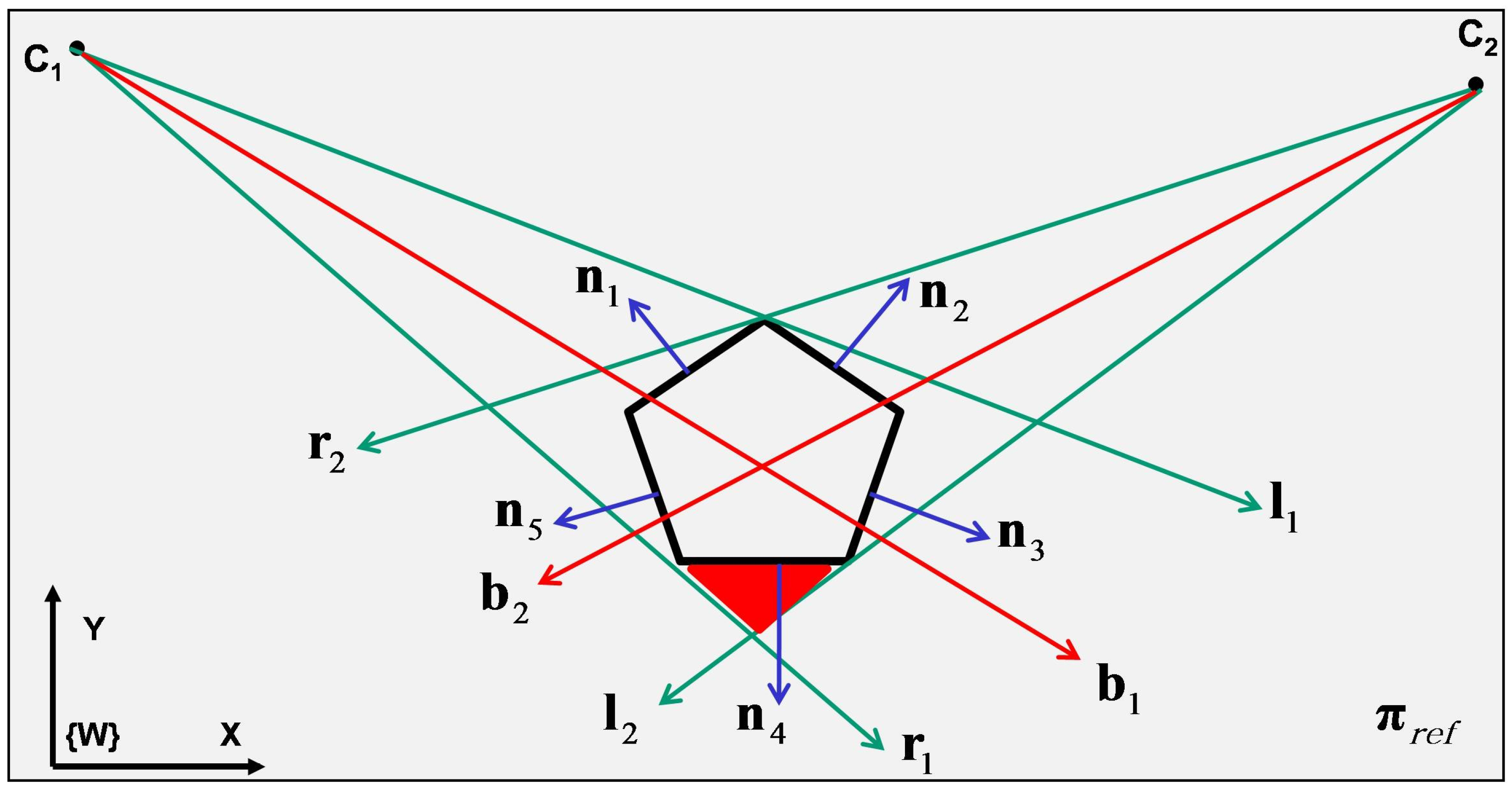
The proposed volumetric reconstruction method uses silhouettes of an object and provides its volumetric reconstruction. The completeness of the reconstructed volume depends to some parameters such as the positions of cameras within the network, number of cameras and the shape of the object. Figure 1a shows an exemplary case where a convex polygon is observed by two cameras (top view). In this case, the polygon has five edges and five vertices (pentagon), however, as is shown in Figure 1b, it is registered on the inertial plane as a six edge polygon, due to the effect of the mentioned parameters (number of cameras and their positions). The extra part of the polygon after registration is shown in red in the figure. As previously mentioned, registration of the cross section of an object with an inertial plane can be thought of as the intersection among all shadows created by cameras, through considering each camera as a light source. Based on this interpretation, the appearance of the red part can be justified: the red part is the area which can not be seen by any camera and is shadowed in all views. We intend to introduce a geometric approach to realize the visibility or invisibility of an edge. Assume a general convex polygon including k vertices and k edges (e.g., consider Figure 2 as an exemplary polygon corresponding to Figure 1). A normal vector can be considered for each edge resulting in . Lets assume a set of cameras . We see that the normal vector at an edge can be used to identify visibility from a camera . Each camera has a pair of tangents (bounding vectors) to the polygon and for each tangents pair a bisecting vector is considered. Having this, the visibility criteria for the edges can be expressed as following: an edge is visible if and only if there is a where , see Algorithm 1. For example, in Figure 2 camera sees edges , and and the normals , make angles greater than with (clockwise angles). Similarly, camera ‘sees‘ edges , and and the normals , make angles greater than with (clockwise angles). The edge is not visible in either of the cameras and its normal makes angles less than with both bisectors , . Thus, Algorithm 1 classifies the edges visibility for a give object.
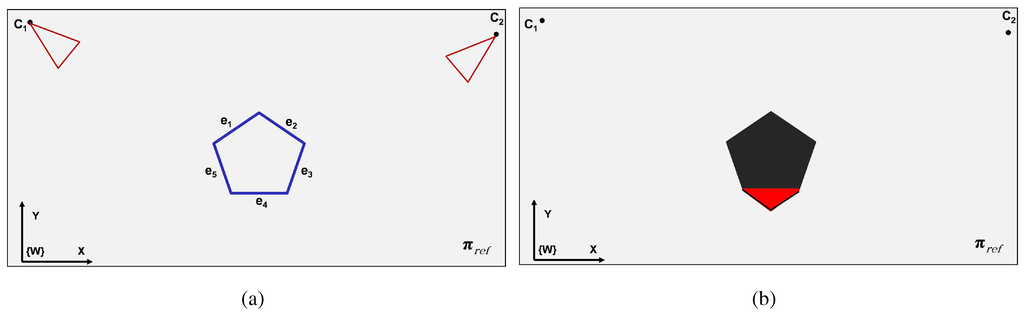
Figure 1.
Investigation of the criteria for visibility of a general convex polygon. (a) An exemplary convex polygon is being observed by two cameras. The images are shown from the top view of the inertial reference plane . (b) The registration of the polygon corresponding to left picture. The registration includes the object and some extra areas (coloured in red) which do not belong to the polygon. This red area has appeared because of not having visibility on the lowest edge of the polygon.
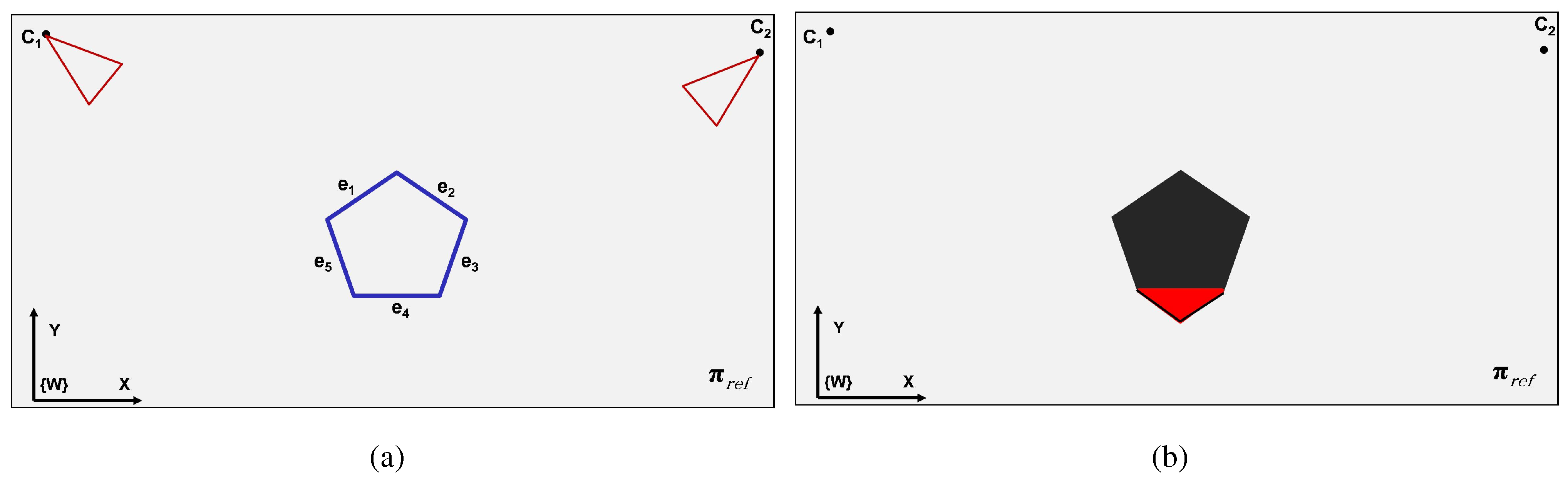
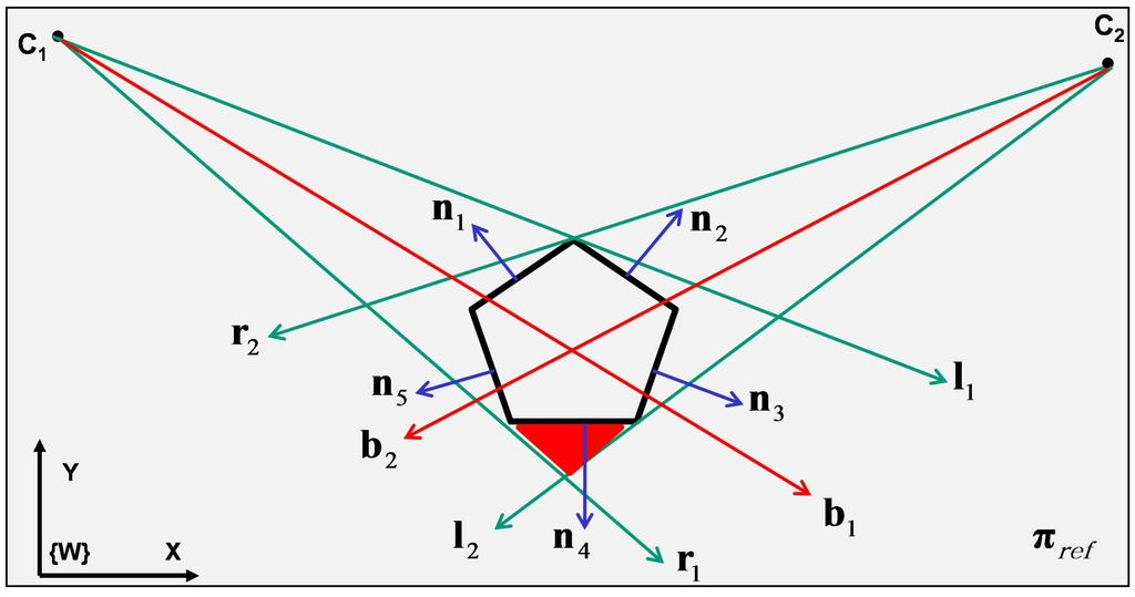
Figure 2.
The figure shows the involved vectors. Green vectors, and , respectively, indicate the left and right tangents (bounding vectors) of a camera . The bisector vector for each camera bounding pair (the tangents) of and is shown in red (). stands for the normal of the edge . After performing the registration process based on the proposed algorithm, the area colored in red also become registered as a part of the object.
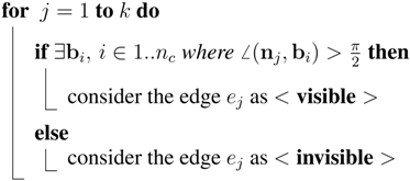
| ALGORITHM 1: Criteria to check the edges visibility for a given polygon. k is number of polygon’s edges and is the j’th edge. is the normal vector corresponding to . is the bisecting vector for camera i. Each edge is checked and will be labelled as either ‘visible’ or ‘invisible’. Labelled as ‘invisible’ for an edge means that it is invisible for all the cameras. |
 |
2.2. Optimal Camera Placement Using Genetic Algorithm
The visibility criteria defined in Algorithm 1 can be used for obtaining an optimal solution for camera placement. The question to be solved is as following: given a convex polygon with k vertices and k edges and number of cameras, what would be an optimal solution for placements of cameras in order to have the best observation of the polygon for applying the proposed reconstruction method. This question can be considered in another form: Given a polygonal space to be monitored by a camera network, what would be an optimal solution to place n cameras around the space. Genetic algorithms (GA) are bio-inspired algorithms, which are known as appropriate mechanisms to solve such a problem. We continue to describe our GA-based algorithm to solve the mentioned problem.
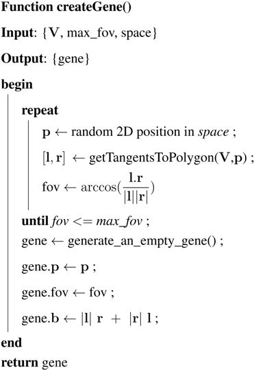
Population in GA is a set of members called chromosome. Each chromosome includes a number of elements named gene. Note that, in our case, a gene is equivalent to a camera and its properties and a chromosome is synonymous to a set of cameras. The structure of a chromosome string is defined in the Table 1. In this structure and stands for the vectors of position and bisector of the camera, fov is the angle of field-of-view (FOV) and cost is an scaler value corresponding to the gene’s cost. Based on these definitions, an algorithm to generate a valid gene is provided in Algorithm 2. The inputs of the algorithm are the vector of vertices of the given polygon, , the search space of the camera positions and maximum possible FOV. Algorithm 3 presents a function to generate a chromosome including genes (a chromosome string with length = ).

Table 1.
Structure of a chromosome string.
| Chromosome | |||||||||||||||
|---|---|---|---|---|---|---|---|---|---|---|---|---|---|---|---|
| gene(1) | gene(2) | ... | gene() | ||||||||||||
| fov | cost | fov | cost | ... | fov | cost | |||||||||
| ALGORITHM 2: Algorithm to generate a valid gene. is the matrix of vertices of the polygon. max_fov is the maximum possible FOV for each gene (camera) and ‘space’ is the search space. Having these as the inputs, the algorithm generates a valid gene with its properties. The position of each gene signifies the position of the corresponding camera. The function getTangentsToPolygon(V,p) receives the matrix of the vertices of the polygon () and the position () of the camera (gene) and returns two vectors ( and ) which are tangents to the given polygon. Then, the angular bisecting vector is stored in . This bisecting vector will be used to compute the cost value of the gene. It can be also interpreted as the looking direction of the camera. Then the generated gene is returned as the result of the function createGene() |
 |
One of the crucial points in GA-based algorithms is to have a suitable cost function in order to evaluate the fitness of a member in the population. In the case of our coverage problem, a cost function is defined (see Figure 4) for a bisector and the normal of an edge as following:
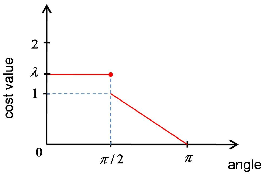
Figure 3.
Defined function to measure the cost between a camera and a polygon edge. The maximum cost is equal to λ and happens when or in other words the edge is invisible by the camera.
Figure 3.
Defined function to measure the cost between a camera and a polygon edge. The maximum cost is equal to λ and happens when or in other words the edge is invisible by the camera.

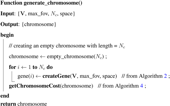
| ALGORITHM 3: Algorithm to generate a chromosome. is the matrix of vertices of the polygon. indicates the chromosome’s length or in other words the number of cameras. max_fov is the maximum possible FOV for each gene (camera) and ‘space’ is the search space. Given these as inputs, the algorithm generate a chromosome with genes and returns it (using Algorithm 2). |
 |
One of the crucial points in GA-based algorithms is to have a suitable cost function in order to evaluate the fitness of a member in the population. In the case of our coverage problem, a cost function is defined (see Figure 4) for a bisector and the normal of an edge as following:
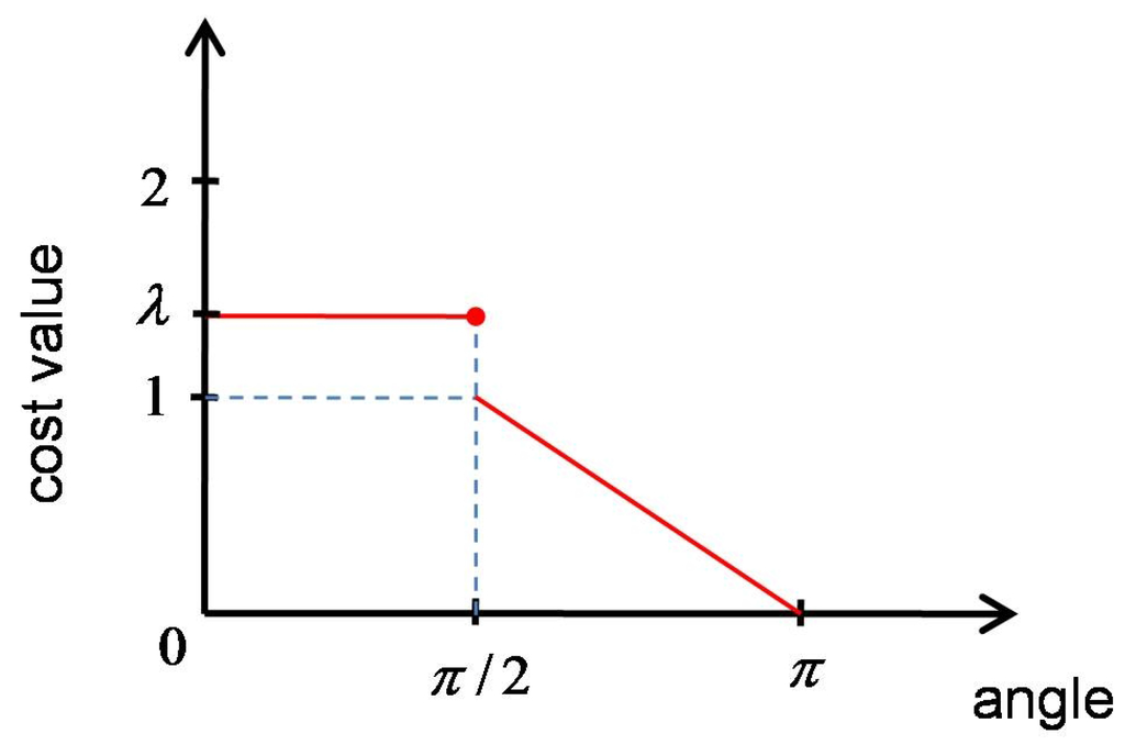
Figure 4.
Defined function to measure the cost between a camera and a polygon edge. The maximum cost is equal to λ and happens when or in other words the edge is invisible by the camera.
Figure 4.
Defined function to measure the cost between a camera and a polygon edge. The maximum cost is equal to λ and happens when or in other words the edge is invisible by the camera.

This causes the genes who are observing the same edges get far from each other and converge other edges.
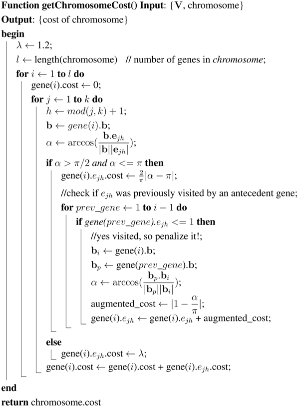
| ALGORITHM 4: Algorithm to compute the cost of a chromosome and its genes. The inputs are , the vertices’s matrix and chromosome. The cost value among each individual gene in the chromosome and each edge of the polygon is computed using the Equation (1). The cost value gets penalized for the genes which are visiting an edge that was previously visited by an antecedent gene of the chromosome (line 0-0). The penalty value is obtained using Equation (2). |
 |
A genetic algorithm (Algorithm 5) to search for an optimal solution is proposed in this section by using the defined cost function and the introduced sub-functions (Algorithms 2–4). The inputs for this algorithm are: V, the matrix of vertices; , maximum for the FOV of a camera (a gene); , number of cameras (number of genes in a chromosome or chromosome’s length); and ’space’, the space to be searched by GA for placing cameras (search space). Number of population (number of chromosomes) is considered as 100. First a new generation is initialized. After applying a fitness function on each individual (chromosomes) in this population, 20% of them are selected as elites for the new generation. The rest of the population (80%) are created by applying crossover and mutation operations on the elites. For doing so, every time two parents are selected randomly from the elites. Then, a crossover operation is applied in this selected couple and as the result two children (new member of the society or chromosomes) are added to the population. On some of the newly created children, a mutation is applied as well. The probability of happening a mutation on the children is considered as . In each cycle, the cost value of the best member (best fitted chromosome) of the elites is saved as the minimum cost value of that generation. If after a number of consecutive trials the cost value does not get improved, or the algorithm reaches its maximum iteration () then it stops. The answer of the algorithm is an optimal chromosome. This optimal solution includes a set of genes ( genes) and each gene signifies a camera with its properties such as position, direction vector, etc.
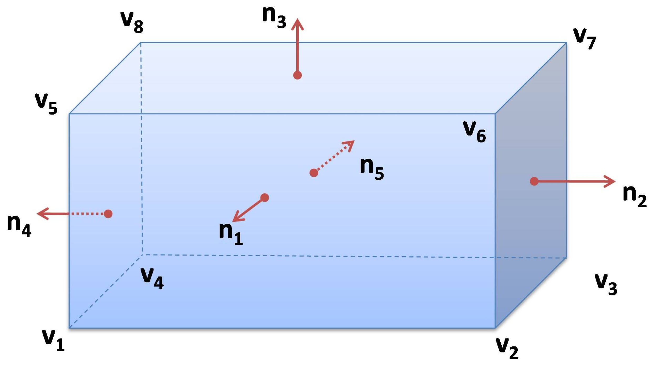
Although the proposed algorithm to optimize the camera coverage is discussed in 2D as a case-study, however it has the potential to be used in 3D with some small modifications. Figure 6 indicates a case where a semi-cube is demonstrated as an exemplary 3D polygon in a 3D space. The first necessary modification in the algorithm to deal with a 3D case is that instead of using the normal vectors of the edges, the normal vectors of the faces have to be used. This counts all faces except the bottom face, which does not need to be observed. The second needed modification is to consider the camera position as 3D instead of 2D, e.g., in Algorithm 2, the place where a camera position in space is randomly created it should be generated as 3D vector. The rest of the algorithm would be the same as the studied 2D case.

Figure 5.
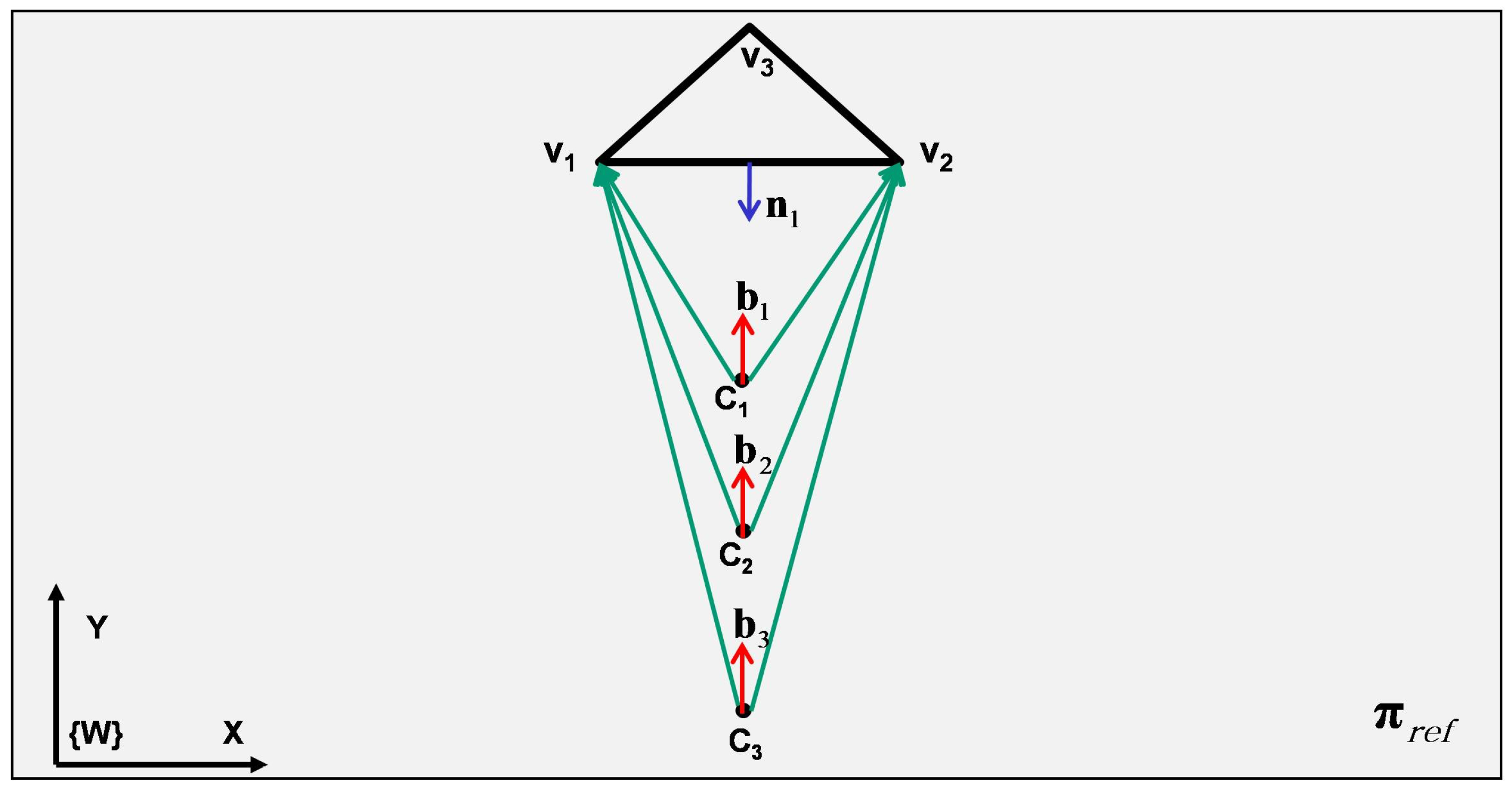
The local minima problem for a triangular polygon and three cameras. Using just the cost value for each gene (camera) regardless of the other genes (cameras) in the same chromosome (camera network) can lead to have one edge perfectly observed by many cameras and other edges lacking. In this case, all three cameras are observing the edge (the line between and ) with cost values at zero since is opposite to their bisector vectors (, and ), whereas the two other edges ( and ) are not observed at all since their cost value can not be zero. The second part of Algorithm 4 is dedicated to eliminating this problem using the penalty function in Equation (2).
Figure 5.
The local minima problem for a triangular polygon and three cameras. Using just the cost value for each gene (camera) regardless of the other genes (cameras) in the same chromosome (camera network) can lead to have one edge perfectly observed by many cameras and other edges lacking. In this case, all three cameras are observing the edge (the line between and ) with cost values at zero since is opposite to their bisector vectors (, and ), whereas the two other edges ( and ) are not observed at all since their cost value can not be zero. The second part of Algorithm 4 is dedicated to eliminating this problem using the penalty function in Equation (2).
| ALGORITHM 5: Genetic algorithm to search for an optimal solution for camera placement problem. |
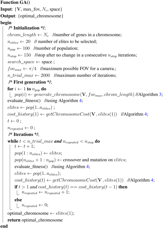 |

Figure 6.
Extension of the proposed algorithm to search for an optimal camera placement from 2D to 3D. In the case of 3D, instead of considering the normals of the edges of the polygon, the normal vectors of the faces must be considered. Moreover, the position part of each gene () must be considered as a 3D vector. The rest of the algorithm would be the same as the 2D case.
3. Camera Placement Optimization Using GAs
3.1. Simulation
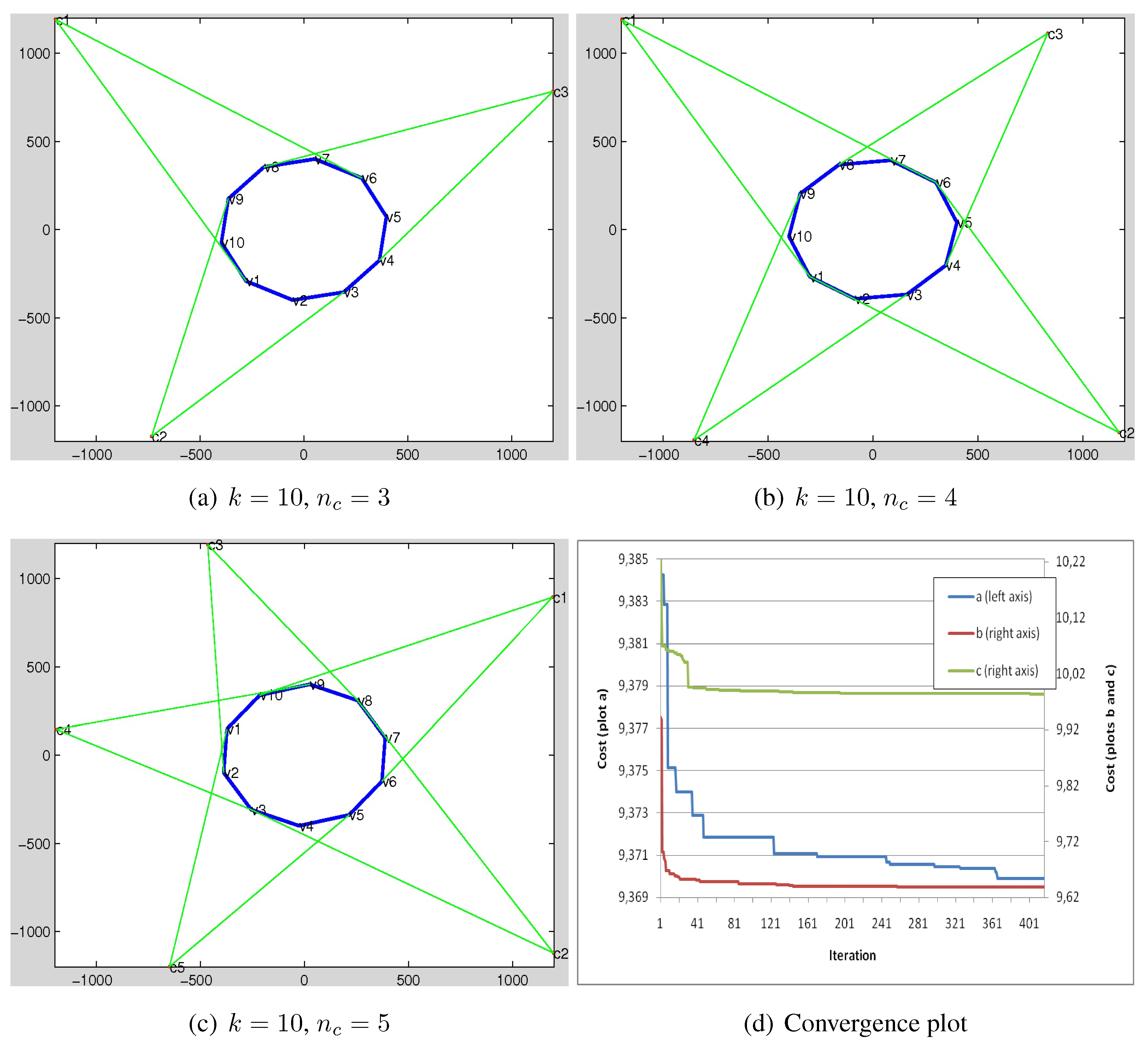
In this section, a set of experiments to demonstrate the efficiency and effectiveness of the proposed GA-based algorithm for camera placement is demonstrated. In total, nine samples are shown in Figure 7, Figure 8 and Figure 9. In each sample a convex polygon with k number of edges and cameras are considered. The polygons are randomly generated and the space to be searched by camera placement has a dimension equal to cm. The convergence plots of the algorithm for the samples in each figure has been depicted in the corresponding (d) section. The vertical axes in the plots show the cost value of the best fittest chromosome in each iteration where the value is divided by number of genes for each sample (number of cameras ).
The condition to stop the GA loop is when the cost values of the found solution in 150 consecutive trials do not improve. As mentioned, the polygon can be either considered as an object to be reconstructed or an area to be observed by the camera network. However, for our case, it is considered as the first case. The proposed GA-based algorithm tries to find an optimal placements (position and direction) of the cameras within the network in such a way that gives the best coverage on the polygon for the purpose of proposed 3D reconstruction method. We next describe a real-world application in coupled camera-intertial sensor network for the purpose of human movements in 3D. We briefly provide the setup and algorithm implementation in GP-GPU and we refer the reader to [22] for more details.

Figure 7.
Results for camera placement optimization using the proposed GA. (a–c) depict three different samples. In each sample, a polygon with k vertices is randomly generated and the purpose of the algorithm is to search for an optimal coverage using number of cameras. The convergences for the samples are plotted in (d). The vertical axis depicts the cost value for the fittest chromosome in each iteration, once it gets divided into the number of genes (). The dimension of the search space is 1200 × 1200 cm.
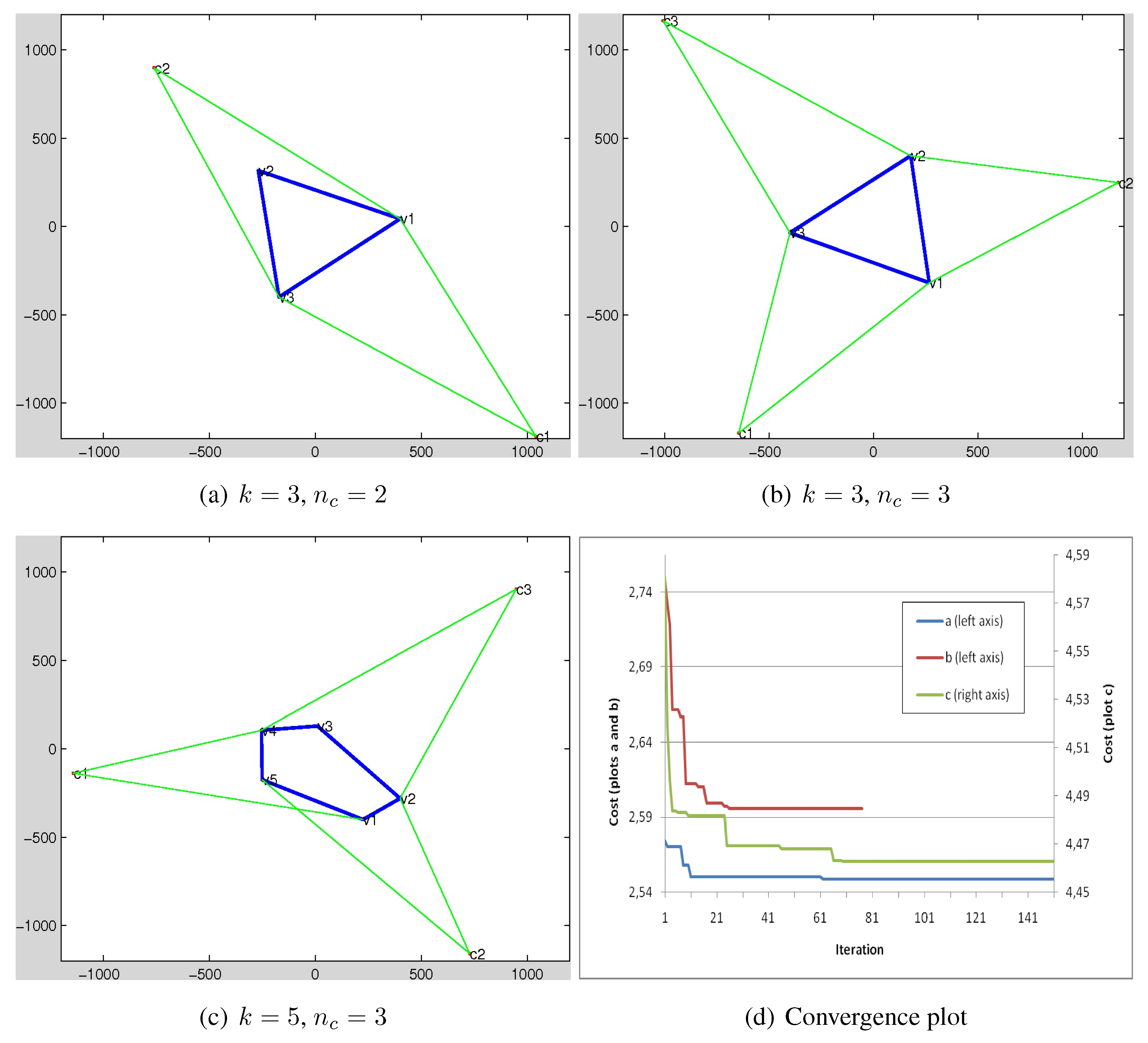

Figure 8.
Results for camera placement optimization using the proposed GA. (a–c) depict three different samples. In each sample, a polygon with k vertices is randomly generated and the purpose of the algorithm is to search for an optimal coverage using number of cameras. The convergences for the samples are plotted in (d). The vertical axis depicts the cost value for the fittest chromosome in each iteration, once it gets divided into the number of genes (). The dimension of the search space is 1200 × 1200 cm.
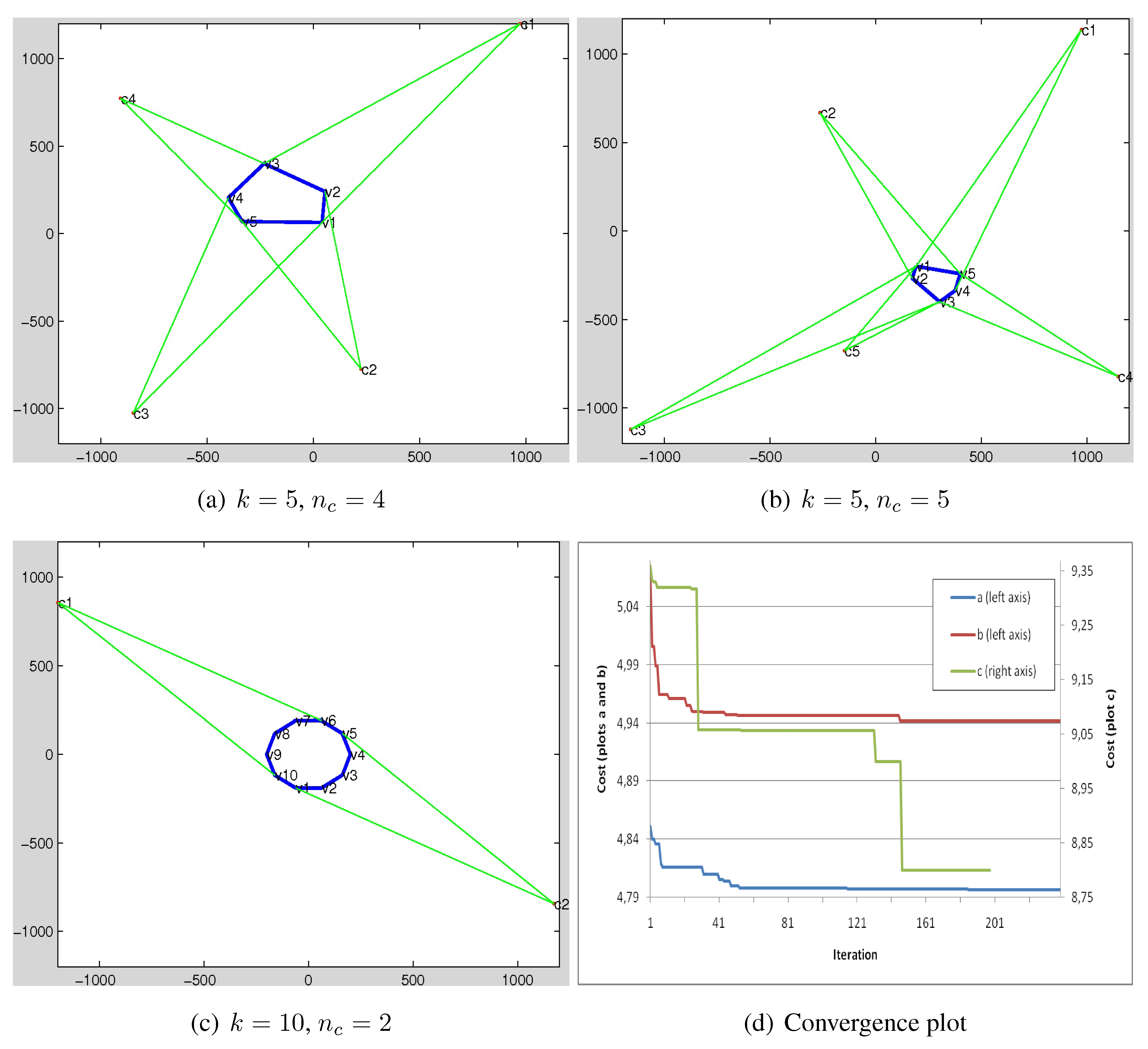
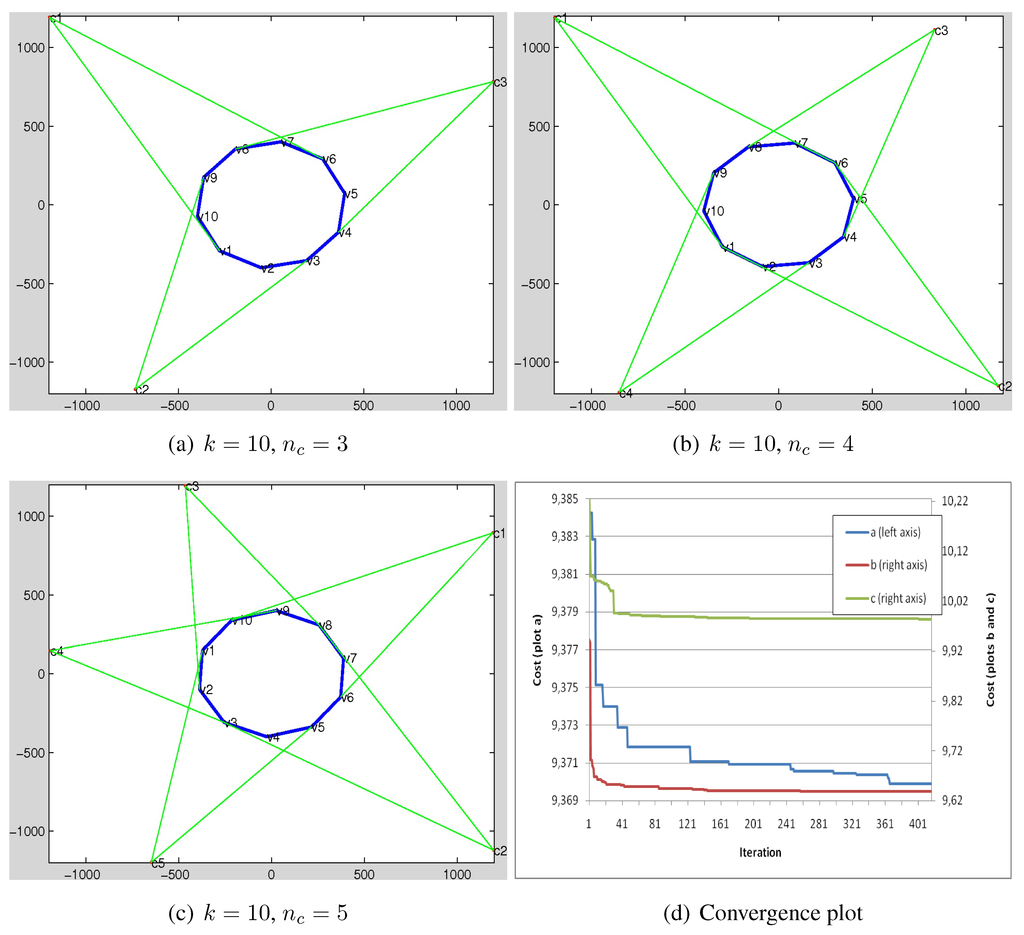
Figure 9.
Results for camera placement optimization using the proposed GA. (a–c) depict three different samples. In each sample, a polygon with k vertices is randomly generated and the purpose of the algorithm is to search for an optimal coverage using number of cameras. The convergences for the samples are plotted in (d). The vertical axis depicts the cost value for the fittest chromosome in each iteration, once it gets divided into the number of genes (). The dimension of the search space is 1200 × 1200 cm.
3.2. Application in 3D Registration for Human Movement Analysis
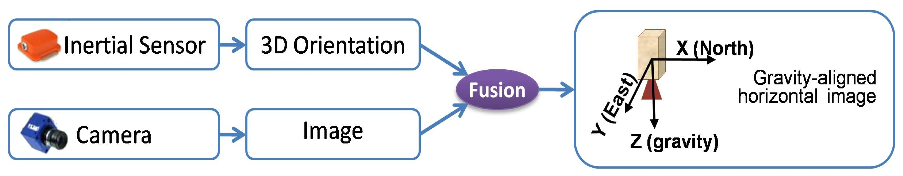
Each coupled system of Camera + Inertial Sensor can be thought of as a virtual camera where the camera provides the visual imagery whereas the inertial sensor gives 3D orientation, see Figure 10 for the experimental setup used in our paper. We utilized AVT Prosilica GC650C cameras coupled with Xsens MTx inertial sensors mounted on the wall. The inertial unit has several type of physical units such as gyroscope, accelerometer, gravity sensor, and compass. Some of the inertial sensors like the one we used (Xsens) have an internal fusion algorithm which combines all measurements from its physical units (specially gravity sensor and compass for our case) and estimates the 3D orientation of the unit in the world reference system. In our framework, we use such an estimated orientation and obtain a transformation matrix which maps the coordinates of the unit to the world reference [23]. Having the attached camera calibrated with the unit, one can obtain a transformation matrix which maps the camera coordinates to the world coordinate systems. The data from both intertial-camera are then fused to obtain a synergistic virtual sensor and its corresponding co-ordinate system, see Figure 11. The fusion was undertaken using the inertial sensor’s 3D orientation and with camera reference frame using homography transformations [24,25,26,27]. Figure 12 illustrates the 3D registration framework used after the GA-optimized optimal configuration of the coupled smart sensors are placed. Note that we only show one inertial plane in Figure 12b, but the overall 3D registration combines multiple inertial frames which are defined using the orientation given by inertial sensors. We then use infinite homography to use fuse inertial–visual information and parametric homographic linear transformations between different internal planes [28]. A detailed evaluation of the data registration framework as well as several other 3D reconstructions can be found in [29,30].
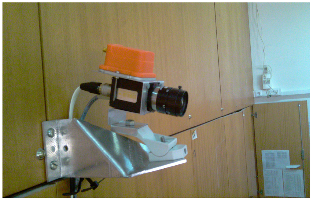
Figure 10.
Experimental setup for a smart sensor. AVT Prosilica GC650C camera coupled with a Xsens MTx inertial sensor mounted on the wall. We setup a network of these smart sensors around the room (Videos are available at YouTube https://www.youtube.com/watch?v=rPibqw4cAxc or in the Supplementary file and more details are available at the website: http://sites.google.com/site/hdakbarpour/research).


Figure 11.
Virtual camera via fusion and downward looking co-ordinate system.
Figure 11.
Virtual camera via fusion and downward looking co-ordinate system.
Our main Algorithm for 3D registration and reconstruction is implemented using CUDA enabled GP-GPU [31], thereby it allowed us to obtain objects/person 3D reconstructions in real-time, see Figure 13a. As can be seen from the components run-time break-down, the most expensive part is the image grabbing from the cameras to the load-shift to the GPU memory. Overall, the framework takes 310 microseconds, thereby enabling us to test it on real time. Figure 13b shows the the processing time of main loop cycle time against the number of inertial planes and their sizes (in cm).
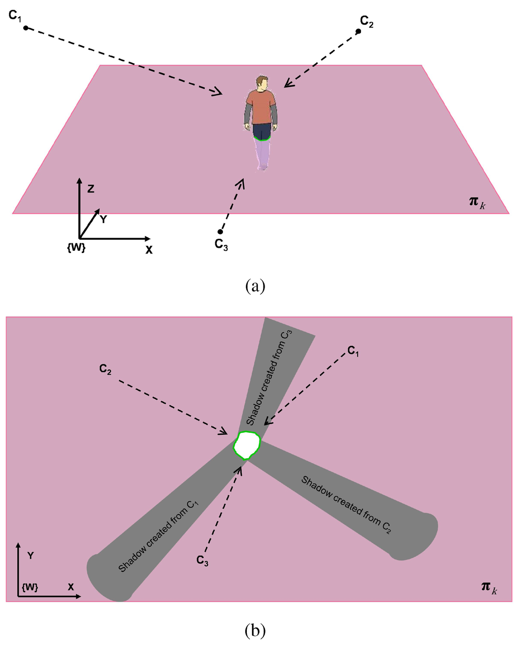
Figure 12.
Illustration of the 3D registration framework using homography concept. (a) A scene including a human and three cameras is depicted. is one inertial-based virtual world plane. The cameras , , and are observing the scene. (b) The registration layer (top view of the plane of (a)). Each camera can be interpreted as a light source and our GA (Algorithm 5) based optimal configuration was used to obtain the final placements and 3D reconstruction experimental results.

We are currently extending and evaluating our system for dynamic scenes, and Figure 14 shows a person walking and the corresponding results capture the motion. Figure 15 shows a screen-grab of our system front-end based on Qt and the movement of a leg is captured. Note that our approach requires neither feature extraction nor availability of ground plane. A higher number of cameras can induce further angle constraints depending upon non-trivial intersections and handling these scenarios within the geometric visibility constraints based GA method is not an easy task. We believe combining a probabilistic framework [8] with our GA optimization is an interesting option and requires further work.
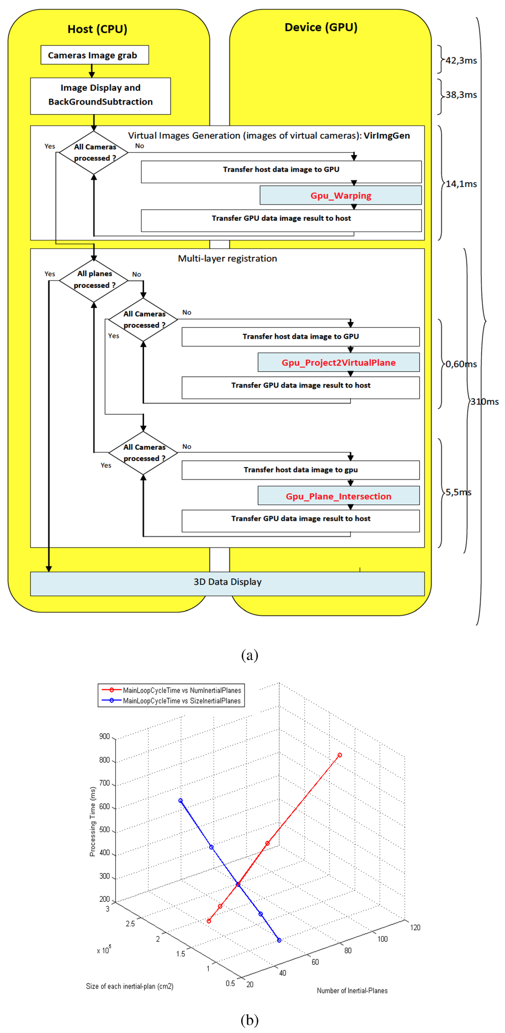
Figure 13.
(a) Our 3D human movement analysis system is implemented using CUDA enabled GP-GPU enabling real-time performance; (b) Processing time with respect to number of inertial Euclidean planes and size () of each inertial planes.
Figure 13.
(a) Our 3D human movement analysis system is implemented using CUDA enabled GP-GPU enabling real-time performance; (b) Processing time with respect to number of inertial Euclidean planes and size () of each inertial planes.

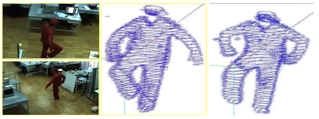
Figure 14.
Dynamic movement of a person under our 3D reconstruction framework.
Figure 14.
Dynamic movement of a person under our 3D reconstruction framework.
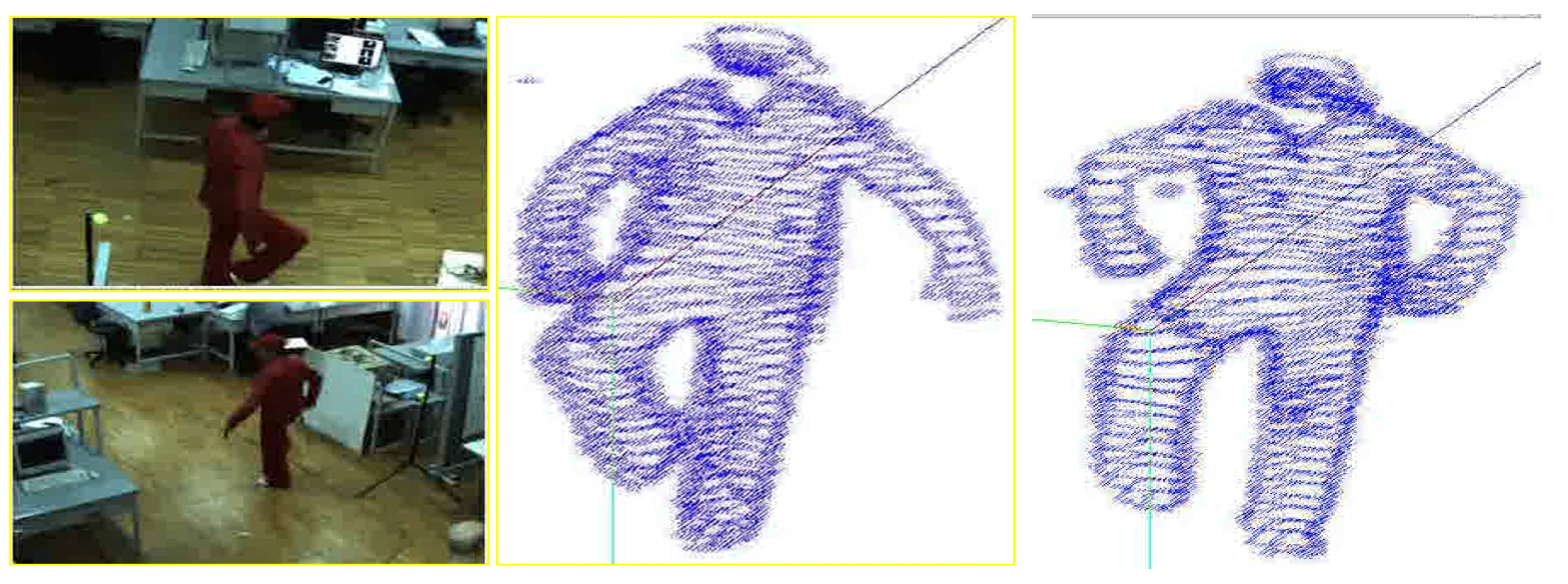
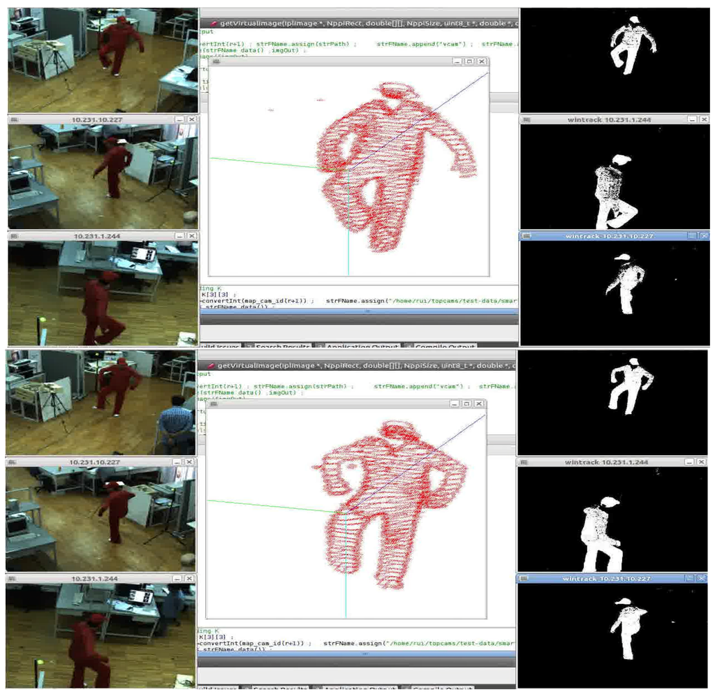
Figure 15.
Online, real-time streaming of our 3D reconstruction results for a dynamic movement of a leg of a person.
Figure 15.
Online, real-time streaming of our 3D reconstruction results for a dynamic movement of a leg of a person.

4. Conclusions
In this work, the coverage problem of cameras within a network of multi-sensors was investigated, in the context of optimal configuration of sensors. Using a geometric cost function, a genetic algorithm was proposed to find an optimal camera configuration in the network. Our geometric cost function based on edge visibility criteria and camera configuration based on visibility vectors is tested on simulated and real smart sensor scenarios. We applied the optimal configuration obtained using our GA based approach for a 3D data registration problem, which involves a network of camera-inertial coupled sensors for human movement analysis. The final pipeline was implemented using CUDA enabled GP-GPU, thereby paving the way for a real-time analysis of 3D data.
Acknowledgments
The authors are grateful to the referees for their constructive remarks which led to improvements in this work. The first author sincerely thanks Luis Almeida from the Institute of Systems and Robotics (ISR), University of Coimbra, Portugal for his help in the project.
Author Contributions
Hadi Aliakbarpour conceived and designed the study under the supervision of Jorge Dias. Both Hadi Aliakbarpour and V. B. Surya Prasath analyzed the results, and Hadi Aliakbarpour, V. B. Surya Prasath, Jorge Dias prepared and revised the paper. This work was carried out at the Jorge Dias’s Mobile Robotics Laboratory at the ISR, University of Coimbra, Portugal. All the authors read and approved the paper.
Conflicts of Interest
The authors declare no conflict of interest.
References
- Aliakbarpour, H.; Freitas, P.; Quintas, J.; Tsiourti, C.; Dias, J. Mobile Robot Cooperation with Infrastructure For Surveillance: Towards Cloud Robotics. In Proceedings of the Workshop on Recognition and Action for Scene Understanding (REACTS) in the 14th International Conference of Computer Analysis of Images and Patterns (CAIP), Malaga, Spain, 1–2 September 2011.
- Blasch, E.; Bosse, E.; Lambert, D.A. High-Level Information Fusion Management and Systems Design; Artech House: Boston, MA, USA, 2012. [Google Scholar]
- Blasch, E.; Plano, S. JDL Level 5 fusion model: User refinement issues and applications in group tracking. SPIE Proc. 2002, 4729, 270–279. [Google Scholar]
- Lohweg, V.; Mönks, U. Sensor fusion by two-layer conflict solving. In Proceedings of the 2010 2nd International Workshop on Cognitive Information Processing (CIP), Elba, Italy, 14–16 June 2010; pp. 370–375.
- Aliakbarpour, H.; Ferreira, J.F.; Khoshhal, K.; Dias, J. A Novel Framework for Data Registration and Data Fusion in Presence of Multi-Modal Sensors. In Emerging Trends in Technological Innovation; Springer: Berlin Heidelberg, Germany, 2010; Volume 314, pp. 308–315. [Google Scholar]
- Xia, S.; Yin, X.; Wu, H.; Jin, M.; Gu, X.D. Deterministic Greedy Routing with Guaranteed Delivery in 3D Wireless Sensor Networks. Axioms 2014, 3, 177–201. [Google Scholar] [CrossRef]
- Kushwaha, M.; Koutsoukos, X. Collaborative 3D Target Tracking in Distributed Smart Camera Networks for Wide-Area Surveillance. J. Sens. Actuator Netw. 2013, 2, 316–353. [Google Scholar] [CrossRef]
- Huber, M. Probabilistic Framework for Sensor Management. Ph.D. Thesis, Fakultät für Informatik, Universität Karlsruhe, Karlsruhe, Germany, 2009. [Google Scholar]
- Bhanu, B.; Ravishankar, V.C.; Roy-Chowdhury, A.K.; Aghajan, H.; Terzopoulos, D. Distributed Video Sensor Networks; Springer: London, UK, 2011. [Google Scholar]
- Zhao, Y.; Wu, H.; Jin, M.; Yang, Y.; Zhou, H.; Xia, S. Cut-and-Sew: A Distributed Autonomous Localization Algorithm for 3D Surface Wireless Sensor Networks. In Proceedings of the 14th ACM International Symposium on Mobile Ad Hoc Networking and Computing (MobiHoc’13), Bangalore, India, 29 July–1 August 2013; pp. 69–78.
- Zhou, H.; Xia, S.; Jin, M.; Wu, H. Localized and Precise Boundary Detection in 3D Wireless Sensor Networks. IEEE/ACM Trans. Netw. (TON) 2015. To appear. [Google Scholar]
- Kavi, R.; Kulathumani, V. Real-Time Recognition of Action Sequences Using a Distributed Video Sensor Network. J. Sens. Actuator Netw. 2013, 2, 486–506. [Google Scholar] [CrossRef]
- Shim, D.S.; Yang, C.K. Optimal Configuration of Redundant Inertial Sensors for Navigation and FDI Performance. Sensors 2010, 10, 6497–6512. [Google Scholar] [CrossRef] [PubMed]
- Yang, C.K.; Shim, D.S. Best Sensor Configuration and Accommodation Rule Based on Navigation Performance for INS with Seven Inertial Sensors. Sensors 2009, 9, 8456–8472. [Google Scholar] [CrossRef] [PubMed]
- Cheng, J.; Dong, J.; Landry, R.J.; Chen, D. A Novel Optimal Configuration form Redundant MEMS Inertial Sensors Based on the Orthogonal Rotation Method. Sensors 2014, 14, 13661–13678. [Google Scholar] [CrossRef] [PubMed]
- Mitchell, M. An Introduction to Genetic Algorithms; MIT Press: Cambridge, MA, USA, 1996. [Google Scholar]
- Ray, P.K.; Mahajan, A. A genetic algorithm-based approach to calculate the optimal configuration of ultrasonic sensors in a 3D position estimation system. Robot. Auton. Syst. 2002, 41, 165–177. [Google Scholar] [CrossRef]
- Biglar, M.; Gromada, M.; Stachowicz, F.; Trzepiecinski, T. Optimal configuration of piezoelectric sensors and actuators for active vibration control of a plate using a genetic algorithm. Acta Mech. 2015, 226, 3451–3462. [Google Scholar] [CrossRef]
- Zhu, N.; O’Connor, I. iMASKO: A Genetic Algorithm Based Optimization Framework for Wireless Sensor Networks. J. Sens. Actuator Netw. 2013, 2, 675–699. [Google Scholar] [CrossRef]
- Liang, W.; Zhang, P.; Chen, X.; Cai, M.; Yang, D. Genetic Algorithm (GA)-Based Inclinometer Layout Optimization. Sensors 2015, 15, 9136–9155. [Google Scholar] [CrossRef] [PubMed]
- Wang, G.; Guo, L.; Duan, H.; Liu, L.; Wang, H. Dynamic Deployment of Wireless Sensor Networks by Biogeography Based Optimization Algorithm. J. Sens. Actuator Netw. 2012, 1, 86–96. [Google Scholar] [CrossRef]
- Aliakbarpour, H.; Aliakbarpour, H.; Naseh, H. 3D Reconstruction of Human/Object Using a Network of Cameras and Inertial Sensors; Scholar’s Press: Saarbrucken, Germany, 2013. [Google Scholar]
- Aliakbarpour, H.; Palaniappan, K.; Dias, J. Geometric exploration of virtual planes in a fusion-based 3D registration framework. In Proceedings of the SPIE Conference Geospatial InfoFusion III (Defense, Security and Sensing: Sensor Data and Information Exploitation), Baltimore, MD, USA, April 2013; Volume 8747.
- Aliakbarpour, H.; Dias, J. IMU-Aided 3D Reconstruction based on Multiple Virtual Planes. In Proceedings of the 2010 International Conference on Digital Image Computing: Techniques and Applications (DICTA), Sydney, NSW, Australia, 1–3 December 2010; pp. 474–479.
- Aliakbarpour, H.; Dias, J. Volumetric 3D reconstruction without planar ground assumption. In Proceedings of the 5th ACM/IEEE Internaltional Conference Distributed Smart Cameras, Ghent, Belgium, 22–25 August 2011.
- Aliakbarpour, H.; Dias, J. Multi-Resolution Virtual Plane Based 3D Reconstruction Using Inertial-Visual Data Fusion. In Proceedings of the International Conference on Computer Vision, Imaging and Computer Graphics Theory and Applications (VISAPP), Vilamoura, Portugal, 5–7 March 2011.
- Aliakbarpour, H.; Dias, J. Inertial-Visual Fusion For Camera Network Calibration. In Proceedings of the 9th IEEE International Conference on Industrial Informatics, Caparica, Lisbon, Portugal, 26–29 July 2011; pp. 422–427.
- Aliakbarpour, H.; Dias, J. Human Silhouette Volume Reconstruction Using a Gravity-Based Virtual Camera Network. In Proceedings of the 13th International Conference on Information Fusion, Edinburgh, UK, 26–29 July 2010.
- Aliakbarpour, H.; Dias, J. Three-dimensional reconstruction based on multiple virtual planes by using fusion-based camera network. IET J. Comput. Vis. 2012, 6, 355–369. [Google Scholar] [CrossRef]
- Aliakbarpour, H. Exploiting Inertial Planes for Multi-Sensor 3D Data Registration. Ph.D. Thesis, University of Coimbra, Coimbra, Portugal, 2012. [Google Scholar]
- Aliakbarpour, H.; Almeida, L.; Menezes, P.; Dias, J. Multi-Sensor 3D Volumetric Reconstruction Using CUDA. J. 3D Res. 2011, 2, 1–14. [Google Scholar] [CrossRef]
© 2015 by the authors; licensee MDPI, Basel, Switzerland. This article is an open access article distributed under the terms and conditions of the Creative Commons Attribution license (http://creativecommons.org/licenses/by/4.0/).